Self-organization of oscillation in an epidemic model for COVID-19

Abstract

On the basis of a compartment model, the epidemic curve is investigated when the net rate $\lambda$ of change of the number of infected individuals $I$ is given by an ellipse in the $\lambda$-$I$ plane which is supported in $[I_{\ell},I_{h}]$. With $a\equiv(I_{h}-I_{\ell})/(I_{h}+I_{\ell})$, it is shown that (1) when $a<1$ or $I_{\ell}>0$, oscillation of the infection curve is self-organized and the period of the oscillation is in proportion to the ratio of the difference $(I_{h}-I_{\ell})$ and the geometric mean $\sqrt{I_{h}I_{\ell}}$ of $I_{h}$ and $I_{\ell}$, (2) when $a=1$, the infection curve shows a critical behavior where it decays obeying a power law function with exponent $-2$ in the long time limit after a peak, and (3) when $a>1$, the infection curve decays exponentially in the long time limit after a peak. The present result indicates that the pandemic can be controlled by a measure which makes $I_{\ell}<0$.

1 Introduction

Since the first outbreak in China in November 2019, COVID-19 has been spreading in all continents including Antarctica. According to a recent analysis of infection status of 186 countries [1, 2], the time dependence of the daily confirmed new cases in more than 80 countries show oscillations whose periods range from one to five months depending on the country. The period of the oscillation is much shorter than that of Spanish flu in 1918$\sim$1919 which is the result of the mutation of virus, and it is an open question why the infection curve of COVID-19 shows oscillation in some countries.

There have been several compartmental models which explain epidemic oscillations [3, 4, 5]. The simplest idea to explain the oscillation is to introduce a sinusoidal time dependence of parameters of the model. Recently, Greer et al [6] introduced a dynamical model with time-varying births and deaths which shows oscillations of epidemics.

Since the infection curve of COVID-19 shows different features depending on the country, the infection curve must have a strong relation to the government policy, and the conventional approach may not be appropriate to COVID-19. In fact, different measures have been employed in each country by its government and citizens have been restricting the social contact among them, both of which depend on the infection status. Therefore, parameters including transmission coefficient of the virus can be considered to be a function of the infection status, and the non-linear effects due to this dependence must be clarified.

In this paper, I introduce a compartment model in which the net rate $\lambda$ of change of the number of infected individuals $I$ is a function of $I$ and the function is given by an ellipse in the $\lambda$-$I$ plane which is supported in $[I_{\ell},I_{h}]$. Here, $I_{h}$ is the upper limit of the number of infected individuals above which the government does not allow, and $I_{\ell}$ is the lowest value below which the government will lift measures. I show that an oscillatory infection curve can be self-organized when $I_{\ell}>0$ and that the period is determined by the ratio of the difference $I_{h}-I_{\ell}$ and the geometric mean $\sqrt{I_{h}I_{\ell}}$ of $I_{h}$ and $I_{\ell}$. I also show that when $I_{\ell}=0$ the infection curve in the long time limit after a single peak decays following a power law function with exponent -2 and when $I_{\ell}<0$ it decays exponentially in the long time limit.

2 Model country

In most of compartmental models for epidemics, the number of infected individuals $I(t)$ is assumed to obey

$$\frac{dI(t)}{dt}=\lambda I(t).$$ (1)

The net rate of change $\lambda$ of the number of infected individuals is written generally as

$$\lambda=\beta\frac{S}{N}-\gamma-\alpha.$$ (2)

Here, $\beta$ and $\gamma$ are the transmission rate of virus from an infected individual to a susceptible individual and a per capta rate for becoming a recovered non-infectious (including dead) individual (R), respectively, and $S$ and $N$ are the number of susceptible individuals and the total population. In Eq. (2), $\alpha$ is a model-dependent parameter representing different effect of epidemics. In the SIR model [8], it is assumed that no effects other than transmission and recovery are considered and thus $\alpha=0$ is assumed. The SEIR model [9] introduces a compartment of exposed individuals (E), and if one sets $\alpha=(dE/dt)/I$, the basic equation of the SEIR model reduces to Eq. (1).

The SIQR model [10, 11] separates quarantined patients (Q) as a compartment in the population and $\alpha$ in Eq. (1) is given by the quarantine rate $q\equiv\Delta Q(t)/I(t)$ where $\Delta Q(t)$ is the daily confirmed new cases [7]. In the application of the SIQR model to COVID-19, it has been shown that

$$\Delta Q(t)\propto I(t-\tau),$$ (3)

where $\tau$ is a typical value of the waiting time between the infection and quarantine of an infected individual. Therefore, the number of the daily confirmed new cases can be assumed to obey Eq. (1) with the redefined time $t-\tau$. Since $\Delta Q(t)$ is treated as an explicit variable instead of $I(t)$, the SIQR model is relevant to COVID-19.

In this paper, I focus on the time evolution of $I(t)$ governed by Eq. (1) for COVID-19. The transmission coefficient is determined by characteristics of the virus and by government policies for lockdown measure and vaccination and by people’s attitude for social distancing. Medical treatment of infected individuals affects $\gamma$ and the government policy on PCR test changes the quarantine rate. The government policies are determined according to the infection status and therefore the rate of change is considered to be a function of $I(t)$ in Eq. (1).

Here, I consider a model country in which $\lambda$ depends on $I$ through

$$\left(\frac{\lambda}{\lambda_{0}}\right)^{2}+\left(\frac{I-I_{0}}{\Delta}\right)^{2}=1.$$ (4)

This implies that when $I$ becomes large, some policies are employed to reduce $\lambda$ to the negative area so that $I(t)$ begins to decline and when $I$ becomes small enough, then some measures are lifted and $\lambda$ becomes positive again. In fact, the plots of $\lambda(t)$ against $I(t)$ in many countries show similar loops [2]. Note that $\lambda=0$ corresponds to either a maximum or a minimum of the number of infected individuals.

Figure 1 shows this dependence, namely $I_{h}\equiv I_{0}+\Delta$ and $I_{\ell}\equiv I_{0}-\Delta$ are the maximum and minimum of the number of infected individuals set by the policy in the country. When $I_{\ell}<0$, $\lambda$ in the region $I<0$ is not relevant since no infected individuals exist in this region.

Figure 1: The dependence of the net rate $\lambda$ on the number of infected individuals $I$ in a model country.

3 Infection curve and self-organization of oscillation

In order to solve Eq. (1) with Eq. (4), I introduce a variable $x$ through

$$\lambda = \lambda_{0}\cos x,$$ (5)

$$I-I_{0} = \Delta\sin x$$ (6)

and rewrite Eq. (1) as

$$a\frac{dx}{d\tilde{t}}=1+a\sin x,$$ (7)

where $\tilde{t}\equiv\lambda_{0}t$ is the time scaled by $\lambda_{0}^{-1}$ and $a\equiv\Delta/I_{0}\geq 0$ is a parameter of the model. Equation (7) can be solved readily under the initial condition $I(t=0)=I_{0}$:

$$\tilde{t}=\left\{\begin{array}[]{ll}\frac{\displaystyle 2a}{\displaystyle\sqrt{1-a^{2}}}\left[\arctan\frac{\displaystyle\tan(x/2)+a}{\displaystyle\sqrt{1-a^{2}}}-\arctan\frac{\displaystyle a}{\displaystyle\sqrt{1-a^{2}}}\right]&\quad\mbox{when $a<1$},\\ \frac{\displaystyle 2\tan(x/2)}{\displaystyle 1+\tan(x/2)}&\quad\mbox{when $a=1$},\\ \frac{\displaystyle a}{\displaystyle\sqrt{a^{2}-1}}\left[\ln\frac{\displaystyle\tan(x/2)+a-\sqrt{a^{2}-1}}{\displaystyle\tan(x/2)+a+\sqrt{a^{2}-1}}-\ln\frac{\displaystyle a-\sqrt{a^{2}-1}}{\displaystyle a+\sqrt{a^{2}-1}}\right]&\quad\mbox{when $a>1$}.\end{array}\right.$$

The infection curve is given in terms of $\tan(x/2)$ by

$$\frac{I(t)}{I_{0}}=1+\frac{a\tan(x/2)}{1+\tan^{2}(x/2)}.$$ (8)

The infection curves are shown for $a=0.4,0.6,0.8,1$ in Fig. 2(a) and for $a=1,2,4,6$ in Fig. 2(b). Therefore, the infection curve is a periodic function when $a<1$ and a decaying function with a single peak when $a\geq 1$.

(a)                                                        (b)

Figure 2: The infection curve for the model country. (a) When $a<1$, a wavy infection curve is self-organized. (b) When $a>1$ the infection curve is a decaying function with a single peak. The infection curve for $a=1$ shown in both panels obeys a power-law decay in the long time limit after a peak.

Characteristics of the infection curve are in order:
(1) When $a<1$, the infection curve shows a self-organized oscillation which can be characterized as follows:

1. The location of the peak $I_{\rm max}/I_{0}=1+a=I_{h}/I_{0}$ and the bottom $I_{\rm min}/I_{0}=1-a=I_{\ell}/I_{0}$ are given by

   $$\tilde{t}_{\rm max}(n) = \frac{2a}{\sqrt{1-a^{2}}}\arctan\left[\sqrt{\frac{1-a}{1+a}}+(n-1)\pi\right],$$ (9)

   $$\tilde{t}_{\rm min}(n) = \frac{2a}{\sqrt{1-a^{2}}}\arctan\left[\sqrt{\frac{1+a}{1-a}}+(n-1)\pi\right],$$ (10)

   respectively, where $n=1,2,\dots$.

2. Therefore, the period $T$ is given by

   $$T\lambda_{0}=\frac{2\pi a}{\sqrt{1-a^{2}}}=\frac{4\pi(I_{h}-I_{\ell})}{\sqrt{I_{h}I_{\ell}}}.$$ (11)

   Namely, the period is given by the ratio of a half of the difference $\Delta=\frac{I_{h}-I_{\ell}}{2}$ and the geometrical mean $\sqrt{I_{h}I_{\ell}}$ of $I_{h}$ and $I_{\ell}$.

(2) When $a=1$, the infection curve shows a peak, after which it decays to zero. It can be characterized as follows:

1. The infection curve reaches its maximum $I_{\rm max}/I_{0}=2$ at $t\lambda_{0}=1$.

2. In the long time limit, it decays as $t^{-2}$.

(3) When $a>1$, the infection curve shows a peak, after which it decays to zero. It can be characterized as follows:

1. The infection curve reaches its maximum $I_{\rm max}/I_{0}=1+a$ at $t\lambda_{0}=\frac{a}{\sqrt{a^{2}-1}}\ln(a+\sqrt{a^{2}-1})$.

2. The infection curve returns to the initial state $I(t)=I_{0}$ at $t\lambda_{0}=\frac{a}{\sqrt{a^{2}-1}}\ln\frac{a+\sqrt{a^{2}-1}}{a-\sqrt{a^{2}-1}}$.

3. In the long time limit, the effective relaxation time defined by $\tau\equiv-\left(\frac{d\ln I}{dt}\right)^{-1}$ is given by $\tau\lambda_{0}=\frac{a}{\sqrt{a^{2}-1}}$.

Figure 3 shows the period for $a<1$ and the relaxation time for $a>1$ as functions of $a$.

Figure 3: The period when $a<1$ and the relaxation time in the long time behavior when $a>1$ are shown as functions of $a$.

4 Discussion

I have shown that oscillation of the infection curve can be self-organized in the epidemic model described by an ordinary differential equation which exploits the net rate of change Eq. (4) depending on the number of infected individuals. All countries employ their own policy which depends on the infection status of the country and the relation Eq. (4) represents general trend of the policy. Namely, when the number of infected individuals approaches the maximum number acceptable in a country, a strong measure is introduced to make the net rate of change $\lambda$ negative, and the measure will be lifted when the number of infected individuals is considered to be small enough, which makes $\lambda>0$. Therefore, the policy with $I_{\ell}>0$ itself is considered to be the origin of the oscillation of the infection curve and the policy with $I_{\ell}<0$ seems to have succeeded in controlling the pandemic [2]. As an example, I show in Fig. 4(a) the time dependence of daily confirmed new cases in Japan from April 5, 2020 to February 11, 2021 which consists of three waves. Using $\lambda$ determined by fitting the data by piece-wise quadratic functions as shown by the solid curve [2], I show the correlation between $\lambda$ and $\Delta Q$ in Fig. 4(b).

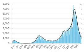
(a)                                               (b)

Figure 4: (a) The time dependence of daily confirmed new cases in Japan from April 5, 2020 to February 11, 2021. The dependence is fitted by piece-wise quadratic functions. (b) The net rate is shown as a function of the number of new cases. The spiral nature of this plot indicates an enhancing wavy behavior of the infection curve. The jumps seen in the plot are due to the procedure which does not impose the continuity of the curvature.

Some of oscillations in biological systems such as the prey and predator system have been explained by the Lotka-Volterra model [12, 13], which is essentially a coupled logistic equation and it is reducible to a second order non-linear differential equation for one variable. Since the present model is based on a first order non-linear differential equation, the origin of oscillatory solution of the present model is different from that of the Lotka-Volterra model.

Several important implications of the present results are:
(1) In order to control the outbreak, a policy is needed to make $a>1$ or $I_{\ell}<0$ and $\lambda<0$. Since $\lambda$ is determined by $\beta$, $S$, $\gamma$ and $\alpha$(or $q$), this can be achieved by the lockdown measure to reduce $\beta$, by the vaccination to reducing $S$ and by the quarantine measure to increase $q$.
(2) The worst policy is $I_{\ell}>0$. In this case, oscillation continues until $\lambda$ becomes negative due to the herd immunity by vaccination and/or infection of a significant fraction of the population.
(3) In order to make $\lambda$ negative, it has been rigorously shown that increasing the quarantine rate $q$ is more efficient than reducing the transmission coefficient $\beta$ by the lockdown measure [14].
This result indicates that the pandemic can be controlled only by keeping measures of $\lambda<0$ till $I=0$.
(4) It should be remarked that the change in the infectivity of the virus due to mutation can be included in $\lambda(I)$ in the present model. Namely effects due to new variants of SARS-CoV-2 found in UK, in South Africa or in Brazil can be included by moving the state to a new $\lambda$ vs $I$ relation.

In this study, I assumed that $I_{0}$ is fixed and the dependence of $\lambda$ on $I$ is symmetric. It is easy to generalize the present formalism to the case of non-symmetric dependence of $\lambda$ on $I$.

Acknowledgments
This work was supported in part by JSPS KAKENHI Grant Number 18K03573.

References

-
[1]
Coronavirus Resource Center, Johns Hopkins University
https://coronavirus.jhu.edu/ - [2] T. Odagaki and R. Suda, https://doi.org/10.1101/2020.12.17.20248445
-
[3]
H. W. Hethcote,
SIAM Rev. 42, 599-653 (2000).
http://doi:10.1137/S0036144500371907 -
[4]
D. J. D. Earn,
Mathematical epidemiology. Lecture Notes in
Mathematics, vol. 1945 (eds. F. Brauer, P. van den Driessche, and J. Wu)
3-17 (Springer, Berlin, Germany, 2008).
https://doi.org/10.1007/978-3-540-78911-6 -
[5]
X. Zhang, C. Shan, Z. Jin and H. Zhu,
J. Differ. Equ. 266, 803-832 (2019).
https://doi:10.1016/j.jde.2018.07.054 -
[6]
M. Greer, R. Saha, A.Gogliettino, C. Yu and K. Zollo-Venecek.
R. Soc. open sci. 7, 191187 (2020).
https://dx.doi.org/10.1098/rsos.191187 -
[7]
T. Odagaki,
Sci. Rep. 11, 1936 (2021).
https://doi.org/10.1038/s41598-021-81521-z -
[8]
W. O. Kermack and A. G. McKendrick,
Proc. Roy. Soc. A 115, 700-721 (1927).
https://doi.org/10.1098/rspa.1932.0171 -
[9]
R. M. Anderson and R. M. May,
Science 215, 1053-1060 (1982).
DOI: 10.1126/science.7063839 -
[10]
H. Hethcote, M. Zhien and L. Shengbing,
Math. Biosciences 180, 141-160 (2002).
https://doi.org/10.1016/S0025-5564(02)00111-6 -
[11]
T. Odagaki,
Infect. Dis. Model. 5, 691-698 (2020).
https://doi:10.1016/j.idm.2020.08.013 -
[12]
A. J. Lotka,
Proc. Natl. Acad. Sci. 6, 410-415 (1920).
https://doi.org/10.1073/pnas.6.7.410 -
[13]
V. Volterra,
Proc. Edin. Math. Soc. 6, 4-10 (1939).
https://doi.org/10.1017/S0013091500008476 -
[14]
T. Odagaki,
Physica A564, 125564–1-9 (2021).
https://doi.org/10.1016/j.physa.2020.125564