The Critical Locus and Rigidity of Foliations of Complex Hénon Maps

Abstract

We study Hénon maps which are perturbations of a hyperbolic polynomial $p$ with connected Julia set. We give a complete description of the critical locus of these maps. In particular, we show that for each critical point $c$ of $p$, there is a primary component of the critical locus asymptotic to the line $y=c$. Moreover, primary components are conformally equivalent to the punctured disk, and their orbits cover the whole critical set. We also describe the holonomy maps from such a component to itself along the leaves of two natural foliations. Finally, we show that a quadratic Hénon map taken along with the natural pair of foliations, is a rigid object, in the sense that a conjugacy between two such maps respecting the foliations is a holomorphic or antiholomorphic affine map.

Preamble

This paper was written in 2005–2006, but has never appeared even as a preprint. Meanwhile, the results have been developed further and have found some applications, see [Fir12, Tan16, FL17]. We are grateful to Tanya Firsova for insisting that this paper should be made available and for helping with the proof reading.

Introduction

The family of Hénon maps are a basic example of nonlinear dynamics. Both the real and the holomorphic versions of these maps have been studied extensively, and yet there is still a great deal that is not well understood about them. Some of the sources of fundamental results about Hénon maps are [FM89], [FS92], [HOV94], [HOV95], [BS91a], [BS91b], [BS92], [BLS93], [BS98a], [BS98b], and [BS99].

In this article we study holomorphic Hénon maps of $\mathbb{C}^{2}$. These are maps of the form

$$f_{a}\begin{pmatrix}x\\ y\end{pmatrix}=\begin{pmatrix}p(x)-ay\\ x\end{pmatrix}$$

where $p$ is a monic polynomial of degree $d>1$. Hénon maps have constant Jacobian, and the parameter $a$ is the value of the Jacobian. In the degenerate case where $a=0$ the map reduces to $f_{0}\begin{pmatrix}x\\ y\end{pmatrix}=\begin{pmatrix}p(x)\\ x\end{pmatrix}$ and we see that the Hénon map degenerates to the polynomial map $p(x)$, acting on the copy of the complex plane given by the curve $x=p(y)$.

The Hénon maps we study here are perturbations of hyperbolic polynomial maps with connected Julia set. The Julia sets and natural foliations of these maps was described in great detail by Hubbard and Oberste-Vorth in [HOV94] and [HOV95]. In this paper we will describe the tangency locus between the natural foliations and will derive from it that the Hénon map endowed with the pair of foliations is a rigid object.

Let us now outline the content of the paper in more detail.

Throughout Section 1 we will recap results of Hubbard & Oberste-Vorth [HOV94] keeping careful track of what happens as the Jacobian of the Hénon map goes to zero. When the Jacobian is equal to zero, the map degenerates, but the foliations and plurisubharmonic functions associated to the map persist, and become easy to analyze.

In Section 2 we present basic facts about the critical locus and, by direct calculation, obtain a description of the tangent spaces to its primary components at infinity.

In Section 3 we recall relevant material from [HOV95] concerning the stable and unstable foliations and describe the critical locus when the Jacobian is zero.

In Section 4 we construct tubes that trap the components of the critical locus as the Jacobian varies away from zero. This allows us to prove that the primary horizontal components of the critical locus are punctured disks. We then show that every component of the critical locus is an iterate of a primary component.

In Section 5 we describe the holonomy maps on a primary horizontal component of the critical locus along the natural foliations.

The pair of natural of foliations of a Hénon map can be thought of as giving natural coordinates near infinity. In Section 6 we prove that if a conjugacy between two Hénon maps in question respects these foliations then it is forced to be holomorphic or antiholomorphic near infinity. For degree two maps, this implies that it is actually affine, which is our main rigidity result.

A list of notations is provided as a reference at the end of the paper. These notations are used with the following convention.

Convention 0.1.

When we extend a certain object from $\mathbb{C}^{2}$ to $\mathbb{P}^{1}\times\mathbb{P}^{1}$ we add a hat to the symbol to distinguish it, unless there is no chance for confusion. When referring to a set with the subset $\{a=0\}$ removed we append the symbol $*$ as a superscript to the symbol denoting that set.

Part I Foliations.

1 The Foliations near Degeneracy

1.1 The Foliations.

In this section we define the foliations associated to a Hénon map. These foliations are not new, they were introduced and studied in [HOV94]. We give a careful development of them from scratch, following the same methods as [HOV94], in order to study what happens in the degenerate case, and to have a good handle on these foliations as the Jacobian $a$ is allowed to vary.

In studying Hénon maps it is common to define domains $V_{+}$ and $V_{-}$ such that $f_{a}(V_{+})\subset V_{+}$ and $f_{a}^{-1}(V_{-})\subset V_{-}$ and such that every point that has unbounded forward orbit eventually enters $V_{+}$ and every point with unbounded backward orbit eventually enters $V_{-}$. We will give precise definitions of these domains shortly.

We first recap the construction of the functions ${\varphi}_{a,\scriptscriptstyle+}\colon V_{+}\to\mathbb{C}$ and ${\varphi}_{a,\scriptscriptstyle-}\colon V_{-}\to\mathbb{C}$, both of which are holomorphic for $a$ in some disk such that ${\varphi}_{a,\scriptscriptstyle+}\circ f_{a}={\varphi}_{a,\scriptscriptstyle+}^{d}$ and ${\varphi}_{a,\scriptscriptstyle+}(x,y)\sim x$ for $|x|>|y|$ as $|x|\to\infty$ and ${\varphi}_{a,\scriptscriptstyle-}\circ f_{a}^{-1}={\varphi}_{a,\scriptscriptstyle-}^{d}/a$ holds for $a\not=0$ and ${\varphi}_{a,\scriptscriptstyle-}(x,y)\sim y$ for $|y|>|x|$ as $|y|\to\infty$.

Throughout this paper it will be convenient to consider the highest term of $p(x)$ separately, thus we write $p(x)=x^{d}+q(x)$ where $d\geq 2$ and $\deg q(x)<d$. We also let ${d^{\prime}}=\deg q(x)$.

We want to construct domains $V_{+}$ and $V_{-}$ where functions ${\varphi}_{a,\scriptscriptstyle+}$ and ${\varphi}_{a,\scriptscriptstyle-}$ are defined for all $a$ in the disk $\mathbb{D}_{R}$ of radius $R$. We will need to control convergence of an infinite product to construct ${\varphi}_{a,\scriptscriptstyle+}$ and ${\varphi}_{a,\scriptscriptstyle-}$ and will choose a value $r$ which will control the rate of convergence of this series.

Fix values $0<r<1$ and $R>0$, and choose $\alpha>0$ such that

• $\Big{\arrowvert}\dfrac{q(y)}{y^{d}}\Big{\arrowvert}+\dfrac{R+1}{|y^{d-1}|}<r$,

• $|p(y)|>(2R+1)|y|$

whenever $|y|\geq\alpha$.

We then define the domains $V_{+}$ and $V_{-}$ to be given by

$$V_{+}\equiv\{(x,y)||x|>|y|\ \text{and}\ |x|>\alpha\},$$

$$V_{-}\equiv\{(x,y)||y|>|x|\ \text{and}\ |y|>\alpha\},$$

We let $\begin{pmatrix}x_{n}\\ y_{n}\end{pmatrix}=f_{a}^{\circ{n}}\begin{pmatrix}x\\ y\end{pmatrix}$ for $n\in\mathbb{Z}$ so $x_{n}$ and $y_{n}$ are polynomial functions in $x$, $y$ and ${\dfrac{1}{a}}$ for $n<0$ and $x_{n}$ and $y_{n}$ are polynomial functions in $x$, $y$ and $a$ for $n>0$.

Lemma 1.1.

Let $a\in\mathbb{D}_{R}$. If $(x,y)\in V_{-}$ then $|x_{-1}|=|y|>|x|$ and $|y_{-1}|>2|y|=2|x_{-1}|$. Thus $f_{a}^{-1}(V_{-})\subset V_{-}$.

Proof.

The statement about $x_{-1}$ is obvious. For $y_{-1}$ we have

$$|y_{-1}|=\big{\arrowvert}\frac{p(y)-x}{a}\big{\arrowvert}\geq\frac{|p(y)|-|y|}{|a|}\geq\frac{2R|y|}{|a|}>2|y|.$$

∎

Lemma 1.2.

Let $a\in\mathbb{D}_{R}$. If $(x,y)\in V_{+}$ then $|y_{1}|=|x|>|y|$ and $|x_{1}|>(R+1)|y_{1}|=(R+1)|x|$. Thus $f_{a}(V_{+})\subset V_{+}$.

Proof.

The statement about $y_{1}$ is obvious. For $x_{1}$ we have

$$|x_{1}|\geq|p(x)|-|ay|\geq|p(x)|-R|x|\geq(R+1)|x|=(R+1)|y_{1}|.$$

∎

1.2 Degeneration of ${\varphi}_{a,\scriptscriptstyle-}$.

We are chiefly interested in the degenerate case ($a=0$) and perturbations of this case ($a$ small). We start by working out the degree of $x_{-k}$ and $y_{-k}$ as polynomials in $y$ and in ${\dfrac{1}{a}}$. In doing so it will be convenient to make the definition $\sigma_{k}=1+d+d^{2}+\dotsb+d^{k-1}$ for $k\geq 1$ and $\sigma_{k}=0$ for $k\leq 0$.

By an easy induction we obtain

Lemma 1.3.

Given that $k\geq 1$ then the leading term of $y_{-k}(x,y,a)$ is

$${\dfrac{1}{a^{\sigma_{k}}}}{\bigl{(}p(y)-x\bigr{)}^{d^{k-1}}}$$

if $y_{-k}$ is considered as a polynomial in $1/a$. The leading term of $y_{-k}(x,y,a)$ considered as a polynomial in $y$ is just the term $y^{d^{k}}/a^{\sigma_{k}}$ of it’s leading term in $\frac{1}{a}$. Since $x_{-k}(x,y,a)=y_{-(k-1)}(x,y,a)$ this also gives us the leading terms of $x_{-k}(x,y,a)$ in $\frac{1}{a}$ and in $y$ except that $x_{-1}(x,y,a)=y$.

The function ${\varphi}_{a,\scriptscriptstyle-}$ is constructed as a limit

$${\varphi}_{a,\scriptscriptstyle-}=\lim_{n\to\infty}(y_{-n}\cdot a^{\sigma_{n}})^{\frac{1}{d^{n}}},$$

with an appropriate choice of the branch of the root. We are interested in this as a function of $V_{-}\times\mathbb{D}_{R}$ where $(x,y)\in V_{-}$ and $a\in\mathbb{D}_{R}$. Sense is made of the above limit using the telescoping formula

$${\varphi}_{a,\scriptscriptstyle-}(x,y)=\lim_{n\to\infty}y\cdot\exp\Bigl{(}\dfrac{1}{d}\log\dfrac{ay_{-1}}{y^{d}}+\dfrac{1}{d^{2}}\log\dfrac{ay_{-2}}{y_{-1}^{d}}+\dotsb\Bigr{)}$$ (1.1)

We are most interested in this about the point $a=0$ (where the map $f_{a}$ degenerates and ${\varphi}_{a,\scriptscriptstyle-}$ can no longer be defined using its relationship with $f_{a}$).

We note that

$$\dfrac{ay_{-k}}{y_{-(k-1)}^{d}}=\dfrac{p(y_{-(k-1)})-x_{-(k-1)}}{y_{-(k-1)}^{d}}=1+\dfrac{q(y_{-(k-1)})-x_{-(k-1)}}{y_{-(k-1)}^{d}}.$$

Let

$${s}^{\scriptscriptstyle-}_{k}(x,y,a)=\dfrac{q(y_{-(k-1)})-x_{-(k-1)}}{y_{-(k-1)}^{d}}.$$ (1.2)

Lemma 1.4.

$|{s}^{\scriptscriptstyle-}_{k}(x,y,a)|<r$ for $x,y\in V_{-},a\in\mathbb{D}_{R},k\geq 1$.

Proof.

We have:

$$|{s}^{\scriptscriptstyle-}_{k}|\leq\dfrac{|q(y_{-(k-1)})|+|x_{-(k-1)}|}{|y_{-(k-1)}^{d}|}\leq\Big{\arrowvert}\dfrac{q(y_{-(k-1)})}{y_{-(k-1)}^{d}}\Big{\arrowvert}+\dfrac{1}{|y_{-(k-1)}^{d-1}|}<r$$

∎

We evaluate $\log{\dfrac{ay_{-k}}{y_{-(k-1)}^{d}}}=\log(1+{s}^{\scriptscriptstyle-}_{k})$ using the principal branch of $\log$. By Lemma 1.4, $\log(1+{s}^{\scriptscriptstyle-}_{k})\leq-\log(1-r)$. Hence the series

$$\frac{1}{d}\log\frac{ay_{-1}}{y^{d}}+\frac{1}{d^{2}}\log\frac{ay_{-2}}{y_{-1}^{d}}+\dotsb$$ (1.3)

converges uniformly and absolutely to a holomorphic function bounded by
${\dfrac{-\log(1-r)}{d-1}}$. Letting $B=(r-1)^{-\frac{1}{d-1}}$, we conclude:

Corollary 1.5.

${\varphi}_{a,\scriptscriptstyle-}$ as defined by equation (1.1) is holomorphic as a function on $V_{-}\times\mathbb{D}_{R}$ with $(x,y)\in V_{-}$ and $a\in\mathbb{D}_{R}$. Moreover $B^{-1}<\Big{\arrowvert}\dfrac{{\varphi}_{a,\scriptscriptstyle-}}{y}\Big{\arrowvert}<B$.

It will be convenient at times to understand the behavior of ${\varphi}_{a,\scriptscriptstyle-}$ in a suitable compactification of $\mathbb{C}^{2}$. By the Riemann Extension Theorem (see e.g. [GR84] page 132),

Corollary 1.6.

Let $\hat{V}_{-}$ denote the union of $V_{-}$ and the line $y=\infty$ in $\mathbb{P}^{1}\times\mathbb{P}^{1}$, with the point $(\infty,\infty)$ excluded. Then ${\dfrac{{\varphi}_{a,\scriptscriptstyle-}}{y}}$ extends holomorphically to $\hat{V}_{-}\times\mathbb{D}_{R}$ and the norm of the extension is bounded above by $B$ and below by $B^{-1}$

Later, when we study the extension of ${\dfrac{{\varphi}_{a,\scriptscriptstyle-}}{y}}$ described above it will be useful to understand the behavior of ${s}^{\scriptscriptstyle-}_{k}$ near infinity. Lemma 1.3 implies:

Lemma 1.7.

Letting $v={\dfrac{1}{y}}$ then ${s}^{\scriptscriptstyle-}_{k}(x,y,a)$ vanishes to order at least $d^{k-1}$ in $v$.

Corollary 1.8.

${\varphi}_{a,\scriptscriptstyle-}(x,y)\sim y$ as $|y|\to\infty$.

Proof.

We know that ${\dfrac{{\varphi}_{a,\scriptscriptstyle-}(x,y)}{y}}=\exp\Bigl{(}{\dfrac{1}{d}}\log(1+{s}^{\scriptscriptstyle-}_{1})+{\dfrac{1}{d^{2}}}\log(1+{s}^{\scriptscriptstyle-}_{2})+\dotsb\Bigr{)}$. Since ${s}^{\scriptscriptstyle-}_{k}$ vanishes in $v$ for all $k$ we see that this infinite sum is a holomorphic function in $V_{-}\times\mathbb{D}_{R}$ that vanishes in $v$. ∎

Let us now study the behavior of $a\mapsto{\varphi}_{a,\scriptscriptstyle-}$ near $a=0$.

Lemma 1.9.

${s}^{\scriptscriptstyle-}_{k}(x,y,a)$ vanishes in $a$ precisely to order

• $(d-{d^{\prime}})\cdot\sigma_{k-1}$ for $q$ nonconstant;

• $d\cdot\sigma_{k-1}-\sigma_{k-2}$ for $q$ constant.

Moreover, ${s}^{\scriptscriptstyle-}_{k}(x,1/v,a)$ vanishes in $v$ precisely to order

• $(d-{d^{\prime}})d^{k-1}$ for $q$ nonconstant.

• $d^{k}-d^{k-2}$ for $q$ constant and $k\geq 2$,

• $d$ for $q$ constant and $k=1$.

Proof.

It follows from Lemma 1.3 that the denominator of ${s}^{\scriptscriptstyle-}_{k}$ is a polynomial in ${\dfrac{1}{a}}$ of degree $d\cdot\sigma_{k-1}$.

The numerator of ${s}^{\scriptscriptstyle-}_{k}$ is a polynomial in ${\dfrac{1}{a}}$ of degree

• ${d^{\prime}}\cdot\sigma_{k-1}$ for $q$ nonconstant;

• $\sigma_{k-2}$ for $q$ constant.

To justify that the highest degree terms in the numerator never cancel, observe that it is impossible for the degree of $q(y_{-(k-1)})$ to match the degree of $x_{-(k-1)}$ as polynomials in $1/a$ except when $k=1$ or when $q$ is constant and $k=2$. It is easy to check that the Lemma still holds in these cases.

The last assertion also easily follows from Lemma 1.3. ∎

Lemma 1.10.

${\varphi}_{a,\scriptscriptstyle-}(x,y)=\bigl{(}p(y)-x\bigr{)}^{\frac{1}{d}}+ah(x,y,a)$ for some holomorphic function $h$ on $V_{-}\times\mathbb{D}_{R}$.

Proof.

According to Lemma 1.9 all ${s}^{\scriptscriptstyle-}_{k}$, $k\geq 2$, vanish at $a=0$ and hence the series (1.3) takes the form ${\dfrac{1}{d}}\log{\dfrac{ay_{-1}}{y^{d}}}+ag(x,y,a)$ for some holomorphic function $g(x,y,a)$ on $V_{-}\times\mathbb{D}_{R}$. Hence by (1.1)

$${\varphi}_{a,\scriptscriptstyle-}(x,y)=y\cdot\exp\Bigl{(}{\dfrac{1}{d}}\log{\dfrac{ay_{1}}{y^{d}}}\Bigr{)}\cdot\exp\bigl{(}ag(x,y,a)\bigr{)}=\bigl{(}p(y)-x\bigr{)}^{\frac{1}{d}}\exp\bigl{(}ag(x,y,a)\bigr{)},$$

and the conclusion follows. ∎

The domain $f_{a}(V_{-})$ swells as $a\to 0$ to include all of $\mathbb{C}^{2}$ except the curve $C(p)$. We make this precise:

Lemma 1.11.

Given $(x,y)\not\in{J}^{\scriptscriptstyle-}_{0}=C(p)$ then $(x,y)\in f_{a}(V_{-})$ for all sufficiently small values $a$. More generally if $K\Subset\mathbb{C}^{2}\setminus C(p)$ then $K\subset f_{a}(V_{-})$ for all sufficiently small $a$.

Proof.

This follows because $(x,y)\in f_{a}(V_{-})$ iff $|p(y)-x|\geq\alpha|a|$ and $|p(y)-x|\geq|y||a|$. ∎

We let $\mathfrak{V}_{k,-}^{\circ}=\{(x,y,a)|(x,y)\in f_{a}^{\circ{k}}(V_{-}),a\in\mathbb{D}_{R}^{*}\}$ and we let $\mathfrak{V}_{k,-}$ be the union of $\mathfrak{V}_{k,-}^{\circ}$ and the set $\{(x,y,0)|(x,y)\not\in C(p)\}$.

Lemma 1.12.

Given $k\geq 1$ then ${\varphi}_{a,\scriptscriptstyle-}^{d^{k}}$ extends from a holomorphic function on $V_{-}$, to a holomorphic function on $\mathfrak{V}_{k,-}$ by defining ${\varphi}_{a,\scriptscriptstyle-}^{d^{k}}(x,y)\equiv a^{\sigma_{k}}{\varphi}_{a,\scriptscriptstyle-}(f_{a}^{-k}(x,y))$ for $a\not=0$ and ${\varphi}_{0,\scriptscriptstyle-}^{d^{k}}(x,y)=\bigl{(}p(y)-x\bigr{)}^{d^{k-1}}$.

Proof.

If $a\not=0$ then we can extend the function ${\varphi}_{a,\scriptscriptstyle-}^{d^{k}}$ to be holomorphic on $f_{a}^{\circ{k}}(V_{-})$ by defining ${\varphi}_{a,\scriptscriptstyle-}^{d^{k}}(x,y)\equiv a^{\sigma_{k}}{\varphi}_{a,\scriptscriptstyle-}(f_{a}^{-k}(x,y))$. This agrees with ${\varphi}_{a,\scriptscriptstyle-}^{d^{k}}$ on $V_{-}$.

According to our definition and Lemma 1.10

$$\begin{split}{\varphi}_{a,\scriptscriptstyle-}^{d^{k}}(x,y)&=a^{\sigma_{k}}{\varphi}_{a,\scriptscriptstyle-}(x_{-k},y_{-k})\\ &=a^{\sigma_{k}}y_{-k}\cdot\Bigl{(}1+{\dfrac{q(y_{-k})-x_{-k}}{y_{-k}^{d}}}\Bigr{)}^{\frac{1}{d}}+a^{1+\sigma_{k}}h(x_{-k},y_{-k})\\ &=a^{\sigma_{k}}y_{-k}(1+{s}^{\scriptscriptstyle-}_{k}(x,y))^{\frac{1}{d}}+a^{1+\sigma_{k}}h(x_{-k},y_{-k})\end{split}$$ (1.4)

for $(x,y,a)\in\mathfrak{V}^{\circ}_{k,-}$. Now $(x_{-k},y_{-k})\in V_{-}$ when $(x,y,a)\in\mathfrak{V}^{\circ}_{k,-}$ and so $y_{-k}\not=0$. Also ${s}^{\scriptscriptstyle-}_{k}(x_{-k},y_{-k})$ is defined and holomorphic since $y_{-k}\not=0$. From Lemma 1.3 we see that $a^{\sigma_{k}}y_{k}$ is a polynomial in $x,y,a$ whose only term not divisible by $a$ is $\bigl{(}p(y)-x\bigr{)}^{d^{k-1}}$. By Lemma 1.9 ${s}^{\scriptscriptstyle-}_{k}$ vanishes in $a$ and so ${\varphi}_{0,\scriptscriptstyle-}^{d^{k}}(x,y)\equiv\bigl{(}p(y)-x\bigr{)}^{d^{k-1}}$ gives a continuous, and therefore, a holomorphic, extension of ${\varphi}_{a,\scriptscriptstyle-}^{d^{k}}$ to $\mathfrak{V}_{k,-}$. ∎

We let both ${J}^{\scriptscriptstyle-}_{0}$ and ${K}^{\scriptscriptstyle-}_{0}$ denote the curve $p(y)-x=0$. It follows from the previous result that this is consistent with the convention that ${J}^{\scriptscriptstyle-}_{a}$ and ${K}^{\scriptscriptstyle-}_{a}$ will denote the sets $J_{-}$ and $K_{-}$ for the parameter value $a$.

1.3 Degeneration of ${\varphi}_{a,\scriptscriptstyle+}$

Here we include the corresponding constructions for forward iterates.

Lemma 1.13.

The leading term of $x_{k}(x,y,a)$ is $x^{d^{k}}$ if $x_{k}$ is considered as a polynomial in $x$. The leading term of $y_{k}(x,y,a)$ is $x^{d^{k-1}}$ as a polynomial in $x$.

Proof.

This follows from an easy induction using $\begin{pmatrix}x_{1}\\ y_{1}\end{pmatrix}=\begin{pmatrix}p(x)-ay\\ x\end{pmatrix}$ and $\begin{pmatrix}x_{k}\\ y_{k}\end{pmatrix}=\begin{pmatrix}p(x_{k-1})-ay_{k-1}\\ x_{k-1}\end{pmatrix}$. ∎

The function ${\varphi}_{a,\scriptscriptstyle+}$ is constructed as a limit ${\varphi}_{a,\scriptscriptstyle+}=\lim_{n\to\infty}{x_{n}}^{\frac{1}{d^{n}}}$ with an appropriate choice of root on the domain $V_{+}\times\mathbb{D}_{R}$. Sense is made of this using the telescoping formula,

$${\varphi}_{a,\scriptscriptstyle+}(x,y)=\lim_{n\to\infty}x\cdot\exp\Bigl{(}{\dfrac{1}{d}}\log{\dfrac{x_{1}}{x^{d}}}+{\dfrac{1}{d^{2}}}\log{\dfrac{x_{2}}{x_{1}^{d}}}+\dotsb\Bigr{)}$$ (1.5)

Letting ${s}^{\scriptscriptstyle+}_{k}=\dfrac{q(x_{k-1})-ay_{k-1}}{x_{k-1}^{d}}$ so ${\dfrac{x_{k}}{x_{k-1}^{d}}}=1+{s}^{\scriptscriptstyle+}_{k}$ we see that

Lemma 1.14.

$|{s}^{\scriptscriptstyle+}_{k}(x,y,a)|<r$ for $(x,y)\in V_{+},a\in\mathbb{D}_{R}$.

Proof.

$$|{s}^{\scriptscriptstyle+}_{k}|<\dfrac{|q(x_{k-1})|+R|y_{k-1}|}{x_{k-1}^{d}}\leq\Big{\arrowvert}\dfrac{q(x_{k-1})}{x_{k-1}^{d}}\Big{\arrowvert}+{\dfrac{R}{|x_{k-1}^{d-1}|}}<r$$

∎

We evaluate $\log{\dfrac{x_{k}}{x_{k-1}^{d}}}=\log(1+{s}^{\scriptscriptstyle+}_{k})$ using the principal branch of $\log$. Since $|{s}^{\scriptscriptstyle+}_{k}|<r$ then $|\log(1+{s}^{\scriptscriptstyle+}_{k})|<-\log(1-r)$ exactly as before for ${s}^{\scriptscriptstyle-}_{k}$. It follows that the series

$${\dfrac{1}{d}}\log{\dfrac{x_{1}}{x^{d}}}+{\dfrac{1}{d^{2}}}\log{\dfrac{x_{2}}{x_{1}^{d}}}+{\dfrac{1}{d^{3}}}\log{\dfrac{x_{3}}{x_{2}^{d}}}+\dotsb$$ (1.6)

converges absolutely and uniformly.

Since $|{\dfrac{1}{d^{k}}}\log{\dfrac{x_{k}}{x_{k-1}^{d}}}|<{\dfrac{-\log(1-r)}{d^{k}}}$ then the infinite sum (1.6) is no larger than $\log B={\dfrac{-\log(1-r)}{d-1}}$. We conclude that

Corollary 1.15.

The function ${\varphi}_{a,\scriptscriptstyle+}$ defined by equation (1.5) is well defined and holomorphic for all $(x,y)\in V_{+}$ and all $a\in\mathbb{D}_{R}$. Additionally $B^{-1}<\Bigl{\arrowvert}{\dfrac{{\varphi}_{a,\scriptscriptstyle+}}{x}}\Bigr{\arrowvert}<B$.

Proof.

The final claim follows immediately from the expression (1.5) and the bounds just derived on the series (1.6). ∎

For the next lemma we consider $\mathbb{C}^{2}$ as lying in $\mathbb{P}^{1}\times\mathbb{P}^{1}$.

Corollary 1.16.

Let $\hat{V}_{+}$ denote the union of $V_{-}$ and the line $x=\infty$ in $\mathbb{P}^{1}\times\mathbb{P}^{1}$, with the point $(\infty,\infty)$ excluded. Then ${\dfrac{{\varphi}_{a,\scriptscriptstyle+}}{x}}$ extends holomorphically to $\hat{V}_{+}\times\mathbb{D}_{R}$ and $B^{-1}\leq\Big{\arrowvert}{\dfrac{{\varphi}_{a,\scriptscriptstyle+}}{x}}\Big{\arrowvert}\leq B$.

Proof.

This follows from the Riemann extension theorem (see e.g. [GR84] page 132). ∎

In order to better understand this extension we will need to understand ${s}^{\scriptscriptstyle+}_{k}$ on this extension. We extract the relevant information in the following lemma.

Lemma 1.17.

Letting $u={\dfrac{1}{x}}$ then ${s}^{\scriptscriptstyle+}_{k}(x,y,a)$ vanishes to order at least $d^{k-1}$ in $u$.

Proof.

Writing ${s}^{\scriptscriptstyle+}_{k}=\dfrac{q\bigl{(}x_{k-1}(1/u,y,a)\bigr{)}-ay_{k-1}(1/u,y,a)}{x_{k-1}^{d}(1/u,y,a)}$ and multiplying the numerator and denominator by $u^{d^{k}}$ this follows from Lemma 1.13. ∎

Corollary 1.18.

${\varphi}_{a,\scriptscriptstyle+}(x,y,a)\sim x$ as $|x|\to\infty$.

Proof.

We know that ${\dfrac{{\varphi}_{a,\scriptscriptstyle+}(x,y)}{x}}=\exp\Bigl{(}{\dfrac{1}{d}}\log(1+{s}^{\scriptscriptstyle+}_{1})+{\dfrac{1}{d^{2}}}\log(1+{s}^{\scriptscriptstyle+}_{2})+\dotsb\Bigr{)}.$ Since ${s}^{\scriptscriptstyle+}_{k}$ vanishes in $u$ for all $k$ we see that this infinite sum is a holomorphic function on $V_{+}\times\mathbb{D}_{R}$ that vanishes in $u$. ∎

We now have an expression for ${\varphi}_{a,\scriptscriptstyle+}$ as $x$ multiplied by the exponent of a uniformly convergent sum of functions which are holomorphic for $(x,y)\in V_{+}$ and $a\in\mathbb{D}_{R}$.

We let $\mathfrak{V}_{k,+}=\{(x,y,a)|f_{a}^{\circ{k}}(x,y)\in V_{+},a\in\mathbb{D}_{R}\}$.

Lemma 1.19.

For each $k\geq 0$ the function ${\varphi}_{a,\scriptscriptstyle+}^{d^{k}}$ extends to a holomorphic function on $\mathfrak{V}_{k,+}$ given by by ${\varphi}_{a,\scriptscriptstyle+}^{d^{k}}\equiv{\varphi}_{a,\scriptscriptstyle+}\circ f_{a}^{k}$. The function ${\varphi}_{0,\scriptscriptstyle+}$ is defined and holomorphic on all of $\mathbb{C}^{2}\setminus{K}^{\scriptscriptstyle+}_{0}$ and is the Böttcher coordinate $b_{p}(x)$ of $p(x)$.

Proof.

Unlike the case of ${\varphi}_{a,\scriptscriptstyle-}$, there is no difficulty in case $a=0$ here. It is immediate that ${\varphi}_{a,\scriptscriptstyle+}$ is holomorphic as a function on $V_{+}\times\mathbb{D}_{R}$. It is clear from the definition that ${\varphi}_{0,\scriptscriptstyle+}$ is the Böttcher coordinate $b_{p}(x)$ of $p(x)$. The rest of the Lemma is obvious. ∎

1.4 The Functions $\mathcal{G}^{\scriptscriptstyle+}_{a}$ and $\mathcal{G}^{\scriptscriptstyle-}_{a}$.

Definition 1.20.

We follow the standard convention that ${U}^{\scriptscriptstyle+}_{a}\equiv\mathbb{C}^{2}\setminus{K}^{\scriptscriptstyle+}_{a}$ and ${U}^{\scriptscriptstyle-}_{a}\equiv\mathbb{C}^{2}\setminus{K}^{\scriptscriptstyle-}_{a}$. We define $\tilde{U}^{+}\equiv\{(x,y,a)|(x,y)\in{U}^{\scriptscriptstyle+}_{a},a\in\mathbb{D}_{R}\}$ and $\tilde{U}^{-}\equiv\{(x,y,a)|(x,y)\in{U}^{\scriptscriptstyle-}_{a},a\in\mathbb{D}_{R}\}$ with the convention that ${U}^{\scriptscriptstyle-}_{0}\equiv\mathbb{C}^{2}\setminus C(p)$.

Lemma 1.21.

The sets $\tilde{U}^{+}$ and $\tilde{U}^{-}$ are open in $\mathbb{C}^{3}$.

Proof.

$\tilde{U}^{+}=\bigcup_{n=0}^{\infty}f^{-n}(V_{+})$ (even when $a=0$) and therefore $\tilde{U}^{+}$ is open. The result follows for $\tilde{U}^{-}$ by a similar construction for $a\not=0$ and by Lemma 1.11 for $a=0$. ∎

Another fact we will want is

Lemma 1.22.

If $p$ is hyperbolic then no point interior to ${K}^{\scriptscriptstyle+}_{0}$ lies in the closure of $\tilde{U}^{+}$.

Proof.

This is a trivial consequence of the fact that any point interior to ${K}^{\scriptscriptstyle+}_{0}$ is attracted to an attracting cycle. ∎

We recall the Green’s functions

$$\mathcal{G}^{\scriptscriptstyle+}_{a}(x,y)\equiv\left\{\begin{array}[]{ll}\log|{\varphi}_{a,\scriptscriptstyle+}(x,y)|&(x,y)\in{U}^{\scriptscriptstyle+}_{a}\\ 0&(x,y)\in{K}^{\scriptscriptstyle+}_{a}\end{array}\right.$$

and

$$\mathcal{G}^{\scriptscriptstyle-}_{a}(x,y)\equiv\left\{\begin{array}[]{ll}\log|{\varphi}_{a,\scriptscriptstyle-}(x,y)|&(x,y)\in{U}^{\scriptscriptstyle-}_{a}\\ {\dfrac{1}{d-1}}\log|a|&(x,y)\in{K}^{\scriptscriptstyle-}_{a}.\end{array}\right.$$

We take the value of $\mathcal{G}^{\scriptscriptstyle-}_{0}(x,y)$ to be $-\infty$ if $(x,y)\in C(p)$, i.e. if $x=p(y)$. These satisfy

$$\mathcal{G}^{\scriptscriptstyle+}_{a}\circ f_{a}=d\cdot\mathcal{G}^{\scriptscriptstyle+}_{a}$$

and

$$\mathcal{G}^{\scriptscriptstyle-}_{a}\circ f_{a}^{-1}=d\cdot\mathcal{G}^{\scriptscriptstyle-}_{a}-\log|a|\quad\text{for $a\not=0$}.$$

This second relation is sometimes more conveniently written

$$\bigl{(}\mathcal{G}^{\scriptscriptstyle-}_{a}-{\dfrac{1}{d-1}}\log|a|\bigr{)}\circ f_{a}^{-1}=d\cdot\bigl{(}\mathcal{G}^{\scriptscriptstyle-}_{a}-{\dfrac{1}{d-1}}\log|a|\bigr{)}.$$

Convention 1.23.

We will sometimes write $\mathcal{G}^{\scriptscriptstyle+}(x,y,a)$ for $\mathcal{G}^{\scriptscriptstyle+}_{a}(x,y)$ and $\mathcal{G}^{\scriptscriptstyle-}(x,y,a)$ for $\mathcal{G}^{\scriptscriptstyle-}_{a}(x,y)$. This will be convenient, for instance, when postcomposing $\mathcal{G}^{\scriptscriptstyle+}$ with function whose output lies in $\mathbb{C}^{2}\times\mathbb{D}_{R}$.

Hubbard & Oberste-Vorth proved that the Green’s functions are continuous when $f_{a}$ is nondegenerate and the same argument gives continuity in $x$, $y$ and $a$ for $\mathcal{G}^{\scriptscriptstyle+}_{a}$ when $a=0$. We extend this to $\mathcal{G}^{\scriptscriptstyle-}_{a}$ when $a=0$.

Theorem 1.24.

The functions $\mathcal{G}^{\scriptscriptstyle+}_{a}(x,y)$ and $\mathcal{G}^{\scriptscriptstyle-}_{a}(x,y)$ are continuous in $x$, $y$ and $a$ for $a\in\mathbb{D}_{R}$.

Proof.

This follows by the same argument as is used in [HOV94] except in the case of $\mathcal{G}^{\scriptscriptstyle-}$ when $a=0$. For $(x^{\prime},y^{\prime})\not\in C(p)$ the continuity of $\mathcal{G}^{\scriptscriptstyle-}_{a}$ at $(x^{\prime},y^{\prime})$ and $a=0$ follows from Lemma 1.12. For $(x^{\prime},y^{\prime})\in C(p)$ more work is required. If we restrict $\mathcal{G}^{\scriptscriptstyle-}_{a}$ to the slice $a=0$ then we already have shown continuity, so we will assume for most of the rest of this proof that $a\not=0$ (so $f_{a}^{-1}$ is defined).

If $f^{-n}(x,y)\in V_{-}$ then $B^{-1}<\big{\arrowvert}{\dfrac{{\varphi}_{a,\scriptscriptstyle-}(x_{-n},y_{-n})}{y_{-n}}}\big{\arrowvert}<B$ by Corollary 1.5. and so $B^{-1}<\big{\arrowvert}{\dfrac{{\varphi}_{a,\scriptscriptstyle-}^{d^{n}}(x,y)}{a^{\sigma_{n}}y_{-n}}}\big{\arrowvert}<B$. Applying $\log$ to the right hand inequality yields $\mathcal{G}^{\scriptscriptstyle-}_{a}(x,y)<{\dfrac{1}{d^{n}}}\log B+{\dfrac{1}{d^{n}}}\log\big{\arrowvert}a^{\sigma_{n}}y_{-n}\big{\arrowvert}$. Now $(x_{-n},y_{-n})=f_{a}^{-n}(x,y)=f_{a}^{-1}(x_{-(n-1)},y_{-(n-1)})=(y_{-(n-1)},{\dfrac{1}{a}}\bigl{(}p(y_{-(n-1)})-x_{-(n-1)}\bigr{)})$. Therefore $y_{-n}={\dfrac{1}{a}}\bigl{(}p(y_{-(n-1)})-y_{-(n-2)}\bigr{)}$ for $n\geq 2$.

We let $z_{-n}\equiv a^{\sigma_{n}}y_{-n}$ from which it follows that

$$z_{-n}=p(z_{-(n-1)},a^{\sigma_{n-1}})-a^{\sigma_{n}-\sigma_{n-2}-1}z_{n-2}\quad\text{for $n\geq 2$.}$$

where $z_{0}=y$ and $z_{-1}=p(y)-x$. Writing our bound for $\mathcal{G}^{\scriptscriptstyle-}_{a}(x,y)$ in terms of $z_{-n}$ we get:

$$\mathcal{G}^{\scriptscriptstyle-}_{a}(x,y)<{\dfrac{1}{d^{n}}}\log B+{\dfrac{1}{d^{n}}}\log\arrowvert z_{-n}\arrowvert$$ (1.7)

if $f_{a}^{-n}(x,y)\in V_{-}$.

We use the convention that $p(x,y)\equiv y^{d}p(x/y)$. Now fix a constant $C>\frac{1}{2}$ to be greater than $(d+1)$ times the absolute value of the largest coefficient of $p(x,y)$. It is then evident that $|p(x,y)|\leq C\max\{|x|^{d},|y|^{d}\}$. Thus from the recursion relation for $z_{-n}$ we have

$$|z_{-n}|\leq\max\{2\cdot\big{\arrowvert}p(z_{-(n-1)},a^{\sigma_{n-1}})\big{\arrowvert},2\cdot\big{\arrowvert}a^{\sigma_{n}-\sigma_{n-2}-1}z_{-(n-2)}\big{\arrowvert}\}$$

$$\leq\max\{2C|z_{-(n-1)}|^{d},2C|a|^{d\cdot\sigma_{n-1}},2|a|^{d^{n-1}+d^{n-2}-1}|z_{-(n-2)}|\}.$$

Let $\epsilon_{v}$ be an arbitrary positive number satisfying $\epsilon_{v}<{\dfrac{1}{2C}}$. Given a point $(x^{\prime},y^{\prime})\in C(p)$ consider the neighborhood

$$\tilde{\mathcal{U}}(\epsilon_{v})\equiv\Bigl{\{}(x,y,a)\Big{\arrowvert}\,|p(y)-x|<\epsilon_{v}^{d},\ |a|<\min\{2C\epsilon_{v}^{d},{\dfrac{1}{2}}\}\ \text{and}\ |a|^{d-1}|y|<C\epsilon_{v}^{d}\Bigr{\}}$$

of $(x^{\prime},y^{\prime},0)\in\mathbb{C}^{2}\times\mathbb{D}_{R}$. Let $\tilde{\mathcal{U}}^{*}(\epsilon_{v})\equiv\tilde{\mathcal{U}}(\epsilon_{v})\cap(\mathbb{C}^{2}\times\mathbb{D}_{R})$ It can be shown by induction that

$$|z_{-n}|<(2C)^{\sigma_{n}}\epsilon_{v}^{d^{n}}\quad\text{for $(x,y,a)\in\tilde{\mathcal{U}}^{*}(\epsilon_{v})$ and $n\geq 1$.}$$ (1.8)

Combining equation (1.7) and equation (1.8) gives $\mathcal{G}^{\scriptscriptstyle-}_{a}(x,y)<{\dfrac{1}{d^{n}}}\log B+{\dfrac{1}{d^{n}}}\log\Big{\arrowvert}(2C)^{\sigma_{n}}\epsilon_{v}^{d^{n}}\Big{\arrowvert}$ if $(x,y,a)\in\tilde{\mathcal{U}}^{*}(\epsilon_{v})$ and $f_{a}^{-n}(x,y)\in V_{-}$. If $(x,y)\not\in{J}^{\scriptscriptstyle-}_{a}$ then $f_{a}^{-n}(x,y)\in V_{-}$ for all sufficiently large $n$ so we can take the limit as $n\to\infty$ and conclude that $\mathcal{G}^{\scriptscriptstyle-}_{a}(x,y)<\log\bigl{(}|2C|^{\frac{1}{d-1}}\epsilon_{v}\bigr{)}$. On the other hand, if $(x,y)\in{J}^{\scriptscriptstyle-}_{a}$ then $\mathcal{G}^{\scriptscriptstyle-}_{a}(x,y)={\dfrac{1}{d-1}}\log|a|$ by definition.

We conclude that given any $M>0$ and any $(x^{\prime},y^{\prime})\in C(p)$ then there is some $\epsilon_{v}$ such that $\mathcal{G}^{\scriptscriptstyle-}_{a}(x,y)<-M$ when $(x,y,a)\in\tilde{\mathcal{U}}^{*}(\epsilon_{v})\setminus{J}^{\scriptscriptstyle-}_{a}$, and some $\epsilon_{a}$ such that if $|a|<\epsilon_{a}$ and $(x,y)\in{J}^{\scriptscriptstyle-}_{a}$ then $\mathcal{G}^{\scriptscriptstyle-}_{a}(x,y)<-M$. Also there is an open subset of $a=0$ about $(x^{\prime},y^{\prime})$ on which the values of $\mathcal{G}^{\scriptscriptstyle-}_{0}$ are always smaller than $-M$. Combining these sets gives a neighborhood of $(x^{\prime},y^{\prime},0)$ on which $\mathcal{G}^{\scriptscriptstyle-}_{a}(x,y)<-M$. Hence $\mathcal{G}^{\scriptscriptstyle-}_{a}$ is continuous in $x$, $y$ and $a$. ∎

Part II The Critical Locus.

2 The Critical Locus near Infinity.

2.1 The Foliations and the Critical Locus.

The fibers of ${\varphi}_{a,\scriptscriptstyle+}$ and ${\varphi}_{a,\scriptscriptstyle-}$ form holomorphic foliations of $V_{+}$ and $V_{-}$ respectively. These foliations naturally extend to much larger sets using dynamics.

Lemma 2.1.

The holomorphic foliations defined by ${\varphi}_{a,\scriptscriptstyle+}$ on $V_{+}$ and ${\varphi}_{a,\scriptscriptstyle-}$ on $V_{-}$ can be extended to all of $\tilde{U}^{+}$ and $\tilde{U}^{-}$ respectively. The resulting foliations, which we denote ${\mathcal{F}}^{\scriptscriptstyle+}_{a}$ and ${\mathcal{F}}^{\scriptscriptstyle-}_{a}$ respectively, are respected by the dynamics.

Proof.

This is a consequence of Lemma 1.12 and Lemma 1.19. ∎

Notation.

We will use ${\mathcal{L}}^{\scriptscriptstyle+}_{a}(z)$ to mean the entire leaf of ${\mathcal{F}}^{\scriptscriptstyle+}_{a}$ passing through $z$, and similarly for ${\mathcal{L}}^{\scriptscriptstyle-}_{a}(z)$. Given a set $B\subset\mathbb{C}^{2}$ and a point $z\in B$, we will use ${\mathcal{L}}^{\scriptscriptstyle+}_{a}(z,B)$ (resp. ${\mathcal{L}}^{\scriptscriptstyle-}_{a}(z,B)$) to denote the connected component of ${\mathcal{L}}^{\scriptscriptstyle+}_{a}(z)\cap B$ (resp. ${\mathcal{L}}^{\scriptscriptstyle-}_{a}(z)$ ) containing $z$.

Definition 2.2.

Given any holomorphic foliation $\mathcal{F}$ on a two dimensional complex manifold $M$ and a point $z\in M$ we will say that a holomorphic function $g$ defined in a neighborhood $N$ of $z$ is a local defining function for $\mathcal{F}$ if for each leaf $\mathcal{L}$ of $\mathcal{F}$, $g$ is constant on each connnect component of $\mathcal{L}\cap N$ and if $\mathbf{d}g$ is never zero.

Given a pair of holomorphic foliations $\mathcal{F}_{1}$ and $\mathcal{F}_{2}$ on a two-dimensional complex manifold, the critical locus $\mathcal{C}$ of $\mathcal{F}_{1}$ and $\mathcal{F}_{2}$ is the complex variety given locally as the zero set (counting multiplicity) of the holomorphic function $h$ satisfying $h\mathbf{d}x\wedge\mathbf{d}y=\mathbf{d}g_{1}\wedge\mathbf{d}g_{2}$ for a pair of local definining functions $g_{1}$ and $g_{2}$ of $\mathcal{F}_{1}$ and $\mathcal{F}_{2}$ respectively. Equivalently $h=\dfrac{\partial{g_{1}}}{\partial{x}}\dfrac{\partial{g_{2}}}{\partial{y}}-\dfrac{\partial{g_{2}}}{\partial{x}}\dfrac{\partial{g_{1}}}{\partial{y}}$ and hence $\mathcal{C}$ is equal to the critical set (counting multiplicity of components) of the map $(x,y)\mapsto\bigl{(}g_{1}(x,y),g_{2}(x,y)\bigr{)}$.

It is straightforward to check that altering the choice of local defining functions for the foliations only results in multiplying $h$ by a nonvanishing holomorphic function. It is clear that the critical locus of a pair of foliations is exactly the set of points on which the foliations are tangent. However, some care must be taken, as it is possible that some components of the critical locus have multipliciy higher than one. An example is given by the foliations with local defining functions $x$ and $x+x^{2}y$. The critical locus is defined by $x^{2}$, which is the $y$ axis, but with multiplicity two. Under the circumstances we are interested in we will be able to verify that every component of the critical locus has multiplicity one. Until that is done we will need to take into account multiplicity of components when dealing with the critical locus.

Definition 2.3.

Let $\mathscr{C}_{a}$ be the critical locus of the foliations ${\mathcal{F}}^{\scriptscriptstyle+}_{a}$ and ${\mathcal{F}}^{\scriptscriptstyle-}_{a}$. It is easy to confirm that $\mathscr{C}_{a}$ is a closed analytic subvariety of ${U}^{\scriptscriptstyle+}_{a}\cap{U}^{\scriptscriptstyle-}_{a}$ invariant under $f_{a}$.

Observe that since we can define ${\varphi}_{a,\scriptscriptstyle+}$ on all of ${U}^{\scriptscriptstyle+}_{a}$ up to local choice of a root then we can define $\log{\varphi}_{a,\scriptscriptstyle+}$ on all of ${U}^{\scriptscriptstyle+}_{a}$ up to local addition of a constant, and therefore $\mathbf{d}\log{\varphi}_{a,\scriptscriptstyle+}$ is a global holomorphic form on ${U}^{\scriptscriptstyle+}_{a}$. Similarly for $\mathbf{d}\log{\varphi}_{a,\scriptscriptstyle-}$ on ${U}^{\scriptscriptstyle-}_{a}$. If we fix $a$ and consider $\mathbf{d}\log{\varphi}_{a,\scriptscriptstyle+}\wedge\mathbf{d}\log{\varphi}_{a,\scriptscriptstyle-}=w_{a}(x,y)\mathbf{d}x\wedge\mathbf{d}y$ we get the same result as if we compute $\mathbf{d}$ with $a$ nonconstant obtaining

$$\mathbf{d}\log{\varphi}_{\scriptscriptstyle+}\wedge\mathbf{d}\log{\varphi}_{\scriptscriptstyle-}\wedge\mathbf{d}a=\tilde{w}(x,y,a)\mathbf{d}x\wedge\mathbf{d}y\wedge\mathbf{d}a$$

in the sense that $\tilde{w}(x,y,a)=w_{a}(x,y)$. Since ${\varphi}_{a,\scriptscriptstyle+}$ and ${\varphi}_{a,\scriptscriptstyle-}$ do not vanish in $\mathbb{C}^{2}$ then $\mathbf{d}\log{\varphi}_{a,\scriptscriptstyle+}\wedge\mathbf{d}\log{\varphi}_{a,\scriptscriptstyle-}\wedge\mathbf{d}a$ and any local branch of $\mathbf{d}{\varphi}_{\scriptscriptstyle+}^{-1}\wedge\mathbf{d}{\varphi}_{\scriptscriptstyle-}^{-d}\wedge\mathbf{d}a$ are just multiples of each other by a nonvanishing holomorphic function. Thus on the common domain of definition $\tilde{w}$ and $w_{a}$ are multiples of each other by a nonvanishing holomorphic function.

Definition 2.4.

The variety defined by $\tilde{w}$ in $\tilde{U}^{+}\cap\tilde{U}^{-}$ will also be called the critical locus and will be denoted by $\mathscr{C}$. For each $a$ it is exactly the locus along which the foliations defined by ${\varphi}_{a,\scriptscriptstyle+}$ and ${\varphi}_{a,\scriptscriptstyle-}$ are tangent, and is equal to $\mathscr{C}_{a}$.

Lemma 2.5.

Assume $X$ is a one dimensional complex variety in $\mathbb{D}^{2}$ and $Y$ is a smooth holomorphic curve in $\mathbb{D}^{2}$. Assume $Y$ is not contained in $X$ and that $z$ is an intersection point of $X$ and $Y$. Let $r\colon\mathbb{D}\to Y$ be a local parameterization of $Y$ about $z$ with $r(0)=z$ and let $h$ be a local defining function for $X$ about $z$. Then the order of contact, or intersection multiplicity, of $X$ and $Y$ at $z$ (counting multiplicity of the components of $Y$ at $z$) is the order of the zero of $h\circ r$ at $0\in\mathbb{D}$.

Proof.

Since everything is local then without loss of generality we can assume that $Y$ is the $y$ axis and $z$ is the origin. Then the intersection multiplicity is

$$(X,Y)=\dim_{\mathbb{C}}\mathcal{O}_{\mathbb{C}^{2},(0,0)}/\bigl{(}x,h(x,y)\bigr{)}=\dim_{\mathbb{C}}\mathcal{O}_{\mathbb{C},0}/\bigl{(}h(x,y)\bigr{)}=$$

$$\dim_{\mathbb{C}}\mathcal{O}_{\mathbb{C},0}/\bigl{(}h(0,y)\bigr{)}=\dim_{\mathbb{C}}\mathbb{C}[y]/(y^{k})=k$$

where $h(0,y)=a_{k}y^{k}+a_{k+1}y^{k+1}+\dotsb$, $a_{k}\not=0$. This is easily seen to be the order of vanishing of $h\circ r$ at zero. ∎

Lemma 2.6.

If the critical locus of a pair of holomorphic foliations in $\mathbb{D}^{2}$ has a singularity at a point $z$ then the leaves of the foliations must have order of contact greater than two at $z$.

Proof.

We can assume without loss of generality that $z$ is the origin, that one foliation is the vertical complex lines, and that the other foliation has local defining function $h$ in a neighborhood of the origin.

One calculates that critical locus is defined by $\dfrac{\partial{h}}{\partial{y}}=0$. If either $\frac{\partial^{2}h}{\partial y^{2}}{\big{\arrowvert}_{0}}\not=0$ or $\frac{\partial^{2}h}{\partial x\partial y}{\big{\arrowvert}_{0}}\not=0$ then $\dfrac{\partial{h}}{\partial{y}}=0$ defines a smooth variety at zero. Hence if the critical locus of the pair of foliations has a singularity at zero then $\frac{\partial^{2}h}{\partial y^{2}}{\big{\arrowvert}_{0}}=0$, and so by lemma 2.5 the leaves of the two foliations have contact of order at least three at zero. ∎

Lemma 2.7.

Given two holomorphic foliations $\mathcal{F}_{1}$ and $\mathcal{F}_{2}$ of a two dimensional complex manifold and their critical locus $\mathcal{C}$ then:

1. Given any point $z\in\mathcal{C}$, the order of contact of the leaves of $\mathcal{F}_{1}$ and $\mathcal{F}_{2}$ at $z$ is one more than the order of contact of the leaf of either foliation with $\mathcal{C}$ at $z$ (counting the multiplicity of components of $\mathcal{C}$).

2. The subset $\mathcal{K}_{k}\subset\mathcal{C}$ of points of $\mathcal{C}$ where the foliations have contact of order at least $k$ is an analytic subset of $\mathcal{C}$.

Proof.

We will confirm both properties locally. Without loss of generality we can assume that $\mathcal{F}_{1}$ is the foliation of $\mathbb{D}^{2}$ by vertical complex lines and $\mathcal{F}_{2}$ is defined by some local defining function $h\colon\mathbb{D}^{2}\to\mathbb{C}$. Assume $z=(z_{1},z_{2})\in\mathbb{D}^{2}$ and parameterize the leaf of $\mathcal{F}_{1}$ through $z$ by $y\mapsto(z_{1},y)$. Then by lemma 2.5 the order of contact between the leaves through $z$ is the order of vanishing of $h(z_{1},y)-h(z_{1},z_{2})$ in $y$ at $y=z_{2}$. This is precisely the smallest $k\in\mathbb{N}$ such that $\frac{\partial^{j}h}{\partial y^{j}}{\big{\arrowvert}_{(z_{1},z_{2})}}=0$ for $j=1,\dotsc,k-1$. However, since $\mathcal{C}$ is defined by $\dfrac{\partial{h}}{\partial{y}}$ we also conclude by lemma 2.5 that the order of contact of the vertical leaf throuth $z$ with $\mathcal{C}$ at $z$ is the vanishing order of $\dfrac{\partial{h}}{\partial{y}}(z_{1},y)$ in $y$ at $y=z_{2}$ which is exactly one less than the vanshing order of $h(z_{1},y)-h(z_{1},z_{2})$ in $y$ at $y=z_{2}$. This completes the proof of part 1.

We also conclude that for each integer $\ell$, the set $\mathcal{K}_{\ell}\subset\mathcal{C}$ is the common zero set of $\frac{\partial^{j}h}{\partial y^{j}}$ for $j=1,\dotsc,\ell-1$. This completes the proof of part 2. ∎

Corollary 2.8.

Assume we are given two holomorphic foliations $\mathcal{F}_{1}$ and $\mathcal{F}_{2}$ defined on some complex two dimensional manifold. Let $\mathcal{C}$ be the critical locus. If the leaves of $\mathcal{F}_{1}$ and $\mathcal{F}_{2}$ have order of contact two at every point of some component $X$ of $\mathcal{C}$ then $X$ is smooth, $X$ meets no other component of $\mathcal{C}$, $X$ is a component of $\mathcal{C}$ with multiplicity one, and $X$ is everywhere transverse to both foliations.

Proof.

Since $\mathcal{C}$ is smooth everywhere the leaves have order of contact two then $X$ is smooth and meets no other component of $\mathcal{C}$ by lemma 2.6. It follows by part 1 of Lemma 2.7 that $X$ must meet each leaf with order of contact one, i.e. $X$ must be transverse to each leaf, and $X$ must have multiplicity one as a component of $\mathcal{C}$. ∎

2.2 The Critical Locus near Infinity.

We consider the critical locus for the extension of $f_{a}$ to $\mathbb{P}^{1}\times\mathbb{P}^{1}$. The map $f_{a}$ is well defined except at $(\infty,\infty)$. The map $f_{a}^{-1}$ is well defined except at $(\infty,\infty)$ or when $a=0$ and $(x,y)\in C(p)$.

The map $f_{a}$ sends the line $y=\infty$ to the line $x=\infty$ and sends the line $x=\infty$ in turn to the point $(\infty,\infty)$ at which $f_{a}$ is undefined. Similarly, the map $f_{a}^{-1}$ sends the line $x=\infty$ to the line $y=\infty$ and sends the line $y=\infty$ in turn to the point $(\infty,\infty)$ at which $f_{a}^{-1}$ is undefined.

In this section we will show that for each critical point $c$ of the polynomial $p$, and for each $a\in\mathbb{D}_{R}$ the critical locus has a branch asymptotic to the curve $y=c$ as $|x|\to\infty$. We will do this by showing that the critical locus (extended to $\mathbb{P}^{1}\times\mathbb{P}^{1}$) contains the point $(\infty,c)$ and by computing the tangent line to the critical locus at $(\infty,c)$.

Because we will be working in $\mathbb{P}^{1}\times\mathbb{P}^{1}\times\mathbb{D}_{R}$ it will be convenient at times to use the coordinate systems $(u,y,a)$ where $u=1/x$ or $(x,v,a)$ where $v=1/y$ instead of using $(x,y,a)$. Corollary 1.16, written using $(u,y,a)$ coordinates, states that

$${h}^{\scriptscriptstyle+}(u,y,a)\equiv\frac{1}{u{\varphi}_{a,\scriptscriptstyle+}(u,y,a)}$$ (2.1)

is holomorphic on $\hat{V}_{+}\times\mathbb{D}_{R}$ and $B^{-1}\leq|{h}^{\scriptscriptstyle+}|\leq B$. Similarly Corollary 1.6, written using $(x,v,a)$ coordinates, states that

$${h}^{\scriptscriptstyle-}(x,v,a)\equiv\frac{1}{v{\varphi}_{a,\scriptscriptstyle-}(x,v,a)}$$ (2.2)

is holomorphic on $\hat{V}_{-}\times\mathbb{D}_{R}$ and $B^{-1}\leq|{h}^{\scriptscriptstyle-}|\leq B$. We find it useful here to write $f_{a}^{-1}$ with input written in the $(u,y,a)$ coordinates, but the output is written in the coordinates $(x,v,a)$, i.e. $f_{a}^{-1}(u,y,a)=(y,{\dfrac{au}{up(y)-1}},a)$.

Let $\hat{\mathfrak{V}}^{*}_{-}=\{(x,y,a)|(x,y)\in f_{a}(\hat{V}_{-}),a\in\mathbb{D}_{R}^{*}\}$ and let

$$\hat{\mathfrak{V}}_{-}=\hat{\mathfrak{V}}^{*}_{-}\cup\Bigl{(}\bigl{(}{U}^{\scriptscriptstyle-}_{0}\cup(\{\infty\}\times\mathbb{C})\bigr{)}\times\{0\}\Bigr{)}\subset\mathbb{P}^{1}\times\mathbb{P}^{1}\times\mathbb{D}_{R}.$$

The set $\hat{\mathfrak{V}}_{-}$ is just the interior of the closure of $\hat{\mathfrak{V}}^{*}_{-}$ in $\mathbb{P}^{1}\times\mathbb{P}^{1}\times\mathbb{D}_{R}$. Then from the recursion relation it follows that ${\varphi}_{a,\scriptscriptstyle-}^{-d}(u,y,a)={\dfrac{u}{up(y)-1}}{h}^{\scriptscriptstyle-}\bigl{(}y,{\dfrac{au}{up(y)-1}},a\bigr{)}$ on $\hat{\mathfrak{V}}^{*}_{-}$. Since both sides of the equality are holomorphic on $\hat{\mathfrak{V}}_{-}$ they are equal on $\hat{\mathfrak{V}}_{-}$.

Therefore

$$\mathbf{d}{\varphi}_{\scriptscriptstyle+}^{-1}(u,y,a)=\bigl{(}{h}^{\scriptscriptstyle+}+u\dfrac{\partial{{h}^{\scriptscriptstyle+}}}{\partial{u}}\bigr{)}\mathbf{d}u+u\dfrac{\partial{{h}^{\scriptscriptstyle+}}}{\partial{y}}\mathbf{d}y+u\dfrac{\partial{{h}^{\scriptscriptstyle+}}}{\partial{a}}\mathbf{d}a\quad\text{on $\hat{V}_{+}\times\mathbb{D}_{R}$.}$$ (2.3)

Also, letting $\lambda=up(y)-1$ we obtain,

$$\mathbf{d}{\varphi}_{\scriptscriptstyle-}^{-d}(u,y,a)=-\lambda^{-2}\cdot{h}^{\scriptscriptstyle-}\circ f_{a}^{-1}\mathbf{d}u\\ -\lambda^{-2}u^{2}p^{\prime}(y)\cdot{h}^{\scriptscriptstyle-}\circ f_{a}^{-1}\mathbf{d}y+\lambda^{-1}u\cdot\dfrac{\partial{{h}^{\scriptscriptstyle-}}}{\partial{x}}\circ f_{a}^{-1}\mathbf{d}y\\ +\lambda^{-1}u\cdot\dfrac{\partial{{h}^{\scriptscriptstyle-}}}{\partial{v}}\circ f_{a}^{-1}\cdot\Bigl{(}\lambda^{-1}u\mathbf{d}a-\lambda^{-2}a\mathbf{d}u-\lambda^{-2}au^{2}p^{\prime}(y)\mathbf{d}y\Bigr{)}\\ +\lambda^{-1}u\cdot\dfrac{\partial{{h}^{\scriptscriptstyle-}}}{\partial{a}}\circ f_{a}^{-1}\mathbf{d}a\quad\text{on $\hat{\mathfrak{V}}_{-}$.}$$ (2.4)

One then calculates

$$\mathbf{d}{\varphi}_{\scriptscriptstyle+}^{-1}\wedge\mathbf{d}{\varphi}_{\scriptscriptstyle-}^{-d}\wedge\mathbf{d}a=\\ \Biggl{(}\bigl{(}{h}^{\scriptscriptstyle+}+u\dfrac{\partial{{h}^{\scriptscriptstyle+}}}{\partial{u}}\bigr{)}\Bigl{(}-\lambda^{-2}u^{2}p^{\prime}(y)\cdot{h}^{\scriptscriptstyle-}\circ f_{a}^{-1}+u\lambda^{-1}\dfrac{\partial{{h}^{\scriptscriptstyle-}}}{\partial{x}}\circ f_{a}^{-1}-\lambda^{-3}au^{3}p^{\prime}(y)\cdot\dfrac{\partial{{h}^{\scriptscriptstyle-}}}{\partial{v}}\circ f_{a}^{-1}\Bigr{)}\\ +u\dfrac{\partial{{h}^{\scriptscriptstyle+}}}{\partial{y}}\Bigl{(}\lambda^{-2}\cdot{h}^{\scriptscriptstyle-}\circ f_{a}^{-1}+au\lambda^{-3}\cdot\dfrac{\partial{{h}^{\scriptscriptstyle-}}}{\partial{v}}\circ f_{a}^{-1}\Bigr{)}\Biggr{)}\mathbf{d}u\wedge\mathbf{d}y\wedge\mathbf{d}a\\ \text{on $\hat{\mathfrak{V}}_{-}\cap(\hat{V}_{+}\times\mathbb{D}_{R})$.}$$ (2.5)

It is easy to show that the domain $\hat{\mathfrak{V}}_{-}\cap(\hat{V}_{+}\times\mathbb{D}_{R})$ contains the plane $u=0$ in $\mathbb{P}^{1}\times\mathbb{P}^{1}\times\mathbb{D}_{R}$.

Corollary 2.9.

The Foliations ${\mathcal{F}}^{\scriptscriptstyle+}_{a}$ and ${\mathcal{F}}^{\scriptscriptstyle-}_{a}$ extend to holomorphic foliations on $\hat{V}_{+}$ and $\hat{\mathfrak{V}}_{-}$ respectively and ${\varphi}_{a,\scriptscriptstyle+}^{-1}$ and ${\varphi}_{a,\scriptscriptstyle-}^{-d}$ are local defining functions for these foliations. In both extended foliations the leaf through $u=0,y=c$ is the line $u=0$ regardless of the value of $a$.

Proof.

Clearly, for each $a\in\mathbb{D}_{R}$, ${\varphi}_{a,\scriptscriptstyle+}^{-1}$ and ${\varphi}_{a,\scriptscriptstyle-}^{-d}$ define the same foliations as ${\varphi}_{a,\scriptscriptstyle+}$ and ${\varphi}_{a,\scriptscriptstyle-}$ on $V_{+}$ and on $\hat{\mathfrak{V}}_{-}\cap({U}^{\scriptscriptstyle-}_{a}\times\{a\})$. Since ${\varphi}_{\scriptscriptstyle+}^{-1}$ and ${\varphi}_{\scriptscriptstyle-}^{-d}$ are holomorphic functions on $\hat{V}_{+}\times\mathbb{D}_{R}$ and $\hat{\mathfrak{V}}_{-}$ which both vanish on $u=0$ by equations (2.1) and (2.2) then we need only confirm that $\mathbf{d}{\varphi}_{a,\scriptscriptstyle+}^{-1}$ and $\mathbf{d}{\varphi}_{a,\scriptscriptstyle-}^{-d}$ do not vanish on $u=0$. But this follows from equations (2.3) and (2.4). ∎

Lemma 2.10.

${h}^{\scriptscriptstyle+}{\big{\arrowvert}_{u=0}}=1$, and $\dfrac{\partial{{h}^{\scriptscriptstyle+}}}{\partial{y}}$ vanishes in $u$ to order at least $d$. Similarly, ${h}^{\scriptscriptstyle-}{\big{\arrowvert}_{v=0}}=1$, and $\dfrac{\partial{{h}^{\scriptscriptstyle-}}}{\partial{x}}$ vanishes in $v$ to order at least $d$.

Proof.

From equation (2.1), equation (1.5) and the definition of ${s}^{\scriptscriptstyle+}_{k}$ we know

$${h}^{\scriptscriptstyle+}=(1+{s}^{\scriptscriptstyle+}_{1})^{-\frac{1}{d}}\exp\bigl{(}-\frac{1}{d^{2}}\log(1+{s}^{\scriptscriptstyle+}_{2})+\dotsb\bigr{)}$$ (2.6)

We know from Lemma 1.17 that if $k\geq 2$ then ${s}^{\scriptscriptstyle+}_{k}$ vanishes to order at least $d$ in $u$.

Since ${s}^{\scriptscriptstyle+}_{1}={\dfrac{q(x)-ay}{x^{d}}}=u^{d}q({\dfrac{1}{u}})-ayu^{d}$ so $\dfrac{\partial{{s}^{\scriptscriptstyle+}_{1}}}{\partial{y}}=-au^{d}$, it follows from equation (2.6) that $\dfrac{\partial{{h}^{\scriptscriptstyle+}}}{\partial{y}}$ vanishes to order at least $d$ in $u$. The claim about ${h}^{\scriptscriptstyle+}{\big{\arrowvert}_{u=0}}$ follows from equation 2.6.

The results for ${h}^{\scriptscriptstyle-}$ are proven similarly. ∎

Corollary 2.11.

The critical locus of the extensions of ${\mathcal{F}}^{\scriptscriptstyle+}_{a}$ and ${\mathcal{F}}^{\scriptscriptstyle-}_{a}$ in $(\hat{V}_{+}\times\mathbb{D}_{R})\cap\hat{\mathfrak{V}}_{-}$ contains the plane $u=0$ with multiplicity two.

Proof.

Since the $v$ coordinate of $f_{a}^{-1}(u,y,a)$ is ${\dfrac{au}{up(y)-1}}$ one concludes from Lemma 2.10 that equation (2.5) is divisible by $u^{2}$. ∎

Corollary 2.11 is one of the reasons these calculations are done so carefully. If we had simply approximated the critical locus at infinity using a Taylor series we could not make this conclusion.

While we need to extend $\mathscr{C}$ to a variety on $(\hat{V}_{+}\times\mathbb{D}_{R})\cap\hat{\mathfrak{V}}_{-}$, the double component $u=0$ is spurious for our purposes. We let $\tilde{w}$ be the holomorphic function satisfying $\mathbf{d}{\varphi}_{\scriptscriptstyle+}^{-1}\wedge\mathbf{d}{\varphi}_{\scriptscriptstyle-}^{-d}\wedge\mathbf{d}a=u^{2}\tilde{w}(u,y,a)\mathbf{d}u\wedge\mathbf{d}y\wedge\mathbf{d}a$. Then the zero set of $\tilde{w}$ gives an extension of $\mathscr{C}$ to $(\hat{V}_{+}\times\mathbb{D}_{R})\cap\hat{\mathfrak{V}}_{-}$. We will abuse notation and refer to the extended variety as $\mathscr{C}$ as well. It will be obvious from the context whether we are using the extension or not. Extending $\mathscr{C}$ automatically extends $\mathscr{C}_{a}$ to $(\hat{V}_{+}\times\mathbb{D}_{R})\cap\hat{\mathfrak{V}}_{-}$ for each $a\in\mathbb{D}_{R}$ since $\mathscr{C}_{a}$ is the zero set of $w_{a}(u,y)\equiv\tilde{w}(u,y,a)$.

Lemma 2.12.

Given $a\in\mathbb{D}_{R}$ and a point $(0,y_{0},a_{0})$ (written in $(u,y,a)$ coordinates) the defining function for $\mathscr{C}$ takes the form $\tilde{w}(u,y,a)=-p^{\prime}(y)-uH$ for some holomorphic function $H$ defined in a neighborhood of $(0,y_{0},a_{0})$. Thus $(0,c,a)$ is in $\mathscr{C}$ iff $c$ is a critical point of $p$. Moreover if $c$ is an order one critical point of $p$ then $\mathscr{C}$ is smooth at $(0,c,a)$ and the tangent plane to $(0,c,a)$ is given by

$$p^{\prime\prime}(c)\mathbf{d}y+C\mathbf{d}u=0$$

for some $C$ depending upon $c$ and $a$.

Proof.

From Lemma 2.10 we can write: ${h}^{\scriptscriptstyle-}\circ f_{a}^{-1}(u,y,a)={h}^{\scriptscriptstyle-}(y,{\dfrac{au}{up(y)-1}},a)=1+uH_{2}$, $\dfrac{\partial{{h}^{\scriptscriptstyle-}}}{\partial{x}}\circ f_{a}^{-1}(u,y,a)=\dfrac{\partial{{h}^{\scriptscriptstyle-}}}{\partial{x}}(y,{\dfrac{au}{up(y)-1}},a)=u^{d}H_{4}$ and $\dfrac{\partial{{h}^{\scriptscriptstyle+}}}{\partial{y}}=u^{d}H_{6}$ for holomorphic functions $H_{2},H_{4}$ and $H_{6}$. From equation (2.5) one obtains $u^{2}\tilde{w}(u,y,a)=(1+uH_{1})\Bigl{(}\{-u^{2}p^{\prime}(y)(1+uH_{2})\}+uH_{3}\cdot u^{d}H_{4}-u^{3}H_{5}\Bigr{)}-u\cdot u^{d}H_{6}\cdot H_{7}=-u^{2}p^{\prime}(y)-u^{3}H_{8}$ where each $H_{i}$ is a function which is holomorphic in a neighborhood of the given $y_{0},a\in\mathbb{D}_{R}$ and for $u$ sufficiently close to zero. Simplifying gives $\tilde{w}(u,y,a)=-p^{\prime}(y)-uH_{8}$ for some holomorphic $H_{8}$. ∎

Theorem 2.13.

If $c$ is an order one critical point of $p$ then the critical locus $\mathscr{C}_{a}$ passes through the point $(0,c,a)$ (written in $(u,y,a)$ coordinates) and is smooth at this point. Moreover ${\varphi}_{a,\scriptscriptstyle+}^{-1}{\big{\arrowvert}_{\mathscr{C}_{a}}}\to\mathbb{C}$ is a local biholomorphism about this point.

Proof.

Smoothness follows directly from Lemma 2.12. Combining equation (2.3) with Lemma 2.10 gives $\mathbf{d}{\varphi}_{a,\scriptscriptstyle+}^{-1}{\big{\arrowvert}_{\mathscr{C}_{a}}}(0,c,a)=\mathbf{d}u$. By Lemma 2.12 this is nondegenerate on the tangent line of $\mathscr{C}_{a}$ at $(0,c,a)$. ∎

3 Stable and Unstable Manifolds

3.1 Crossed Mappings

In this section we recall the definition of and basic results about crossed mappings from [HOV95]. This is a holomorphic version of a standard construction of stable and unstable manifolds such as Theorem 6.4.9 criteria (4) in [KH95]. We will only define degree one crossed mappings, and we will not consider any crossed mappings of degree higher than one in this paper.

Let $B_{1}=U_{1}\times V_{1}$ and $B_{2}=U_{2}\times V_{2}$ be bidisks.

Definition 3.1.

A (degree one) crossed mapping from $B_{1}$ to $B_{2}$ is a triple $(W_{1},W_{2},f)$, where

1. $W_{1}$ is an open subset of $U^{\prime}_{1}\times V_{1}$ for some open $U^{\prime}_{1}\Subset U_{1}$.

2. $W_{2}$ is an open subset of $U_{2}\times V^{\prime}_{2}$ for some open $V^{\prime}_{2}\Subset V_{2}$.

3. $f\colon W_{1}\to W_{2}$ is a holomorphic isomorphism, such that for all $y\in V_{1}$ the mapping

   $$\operatorname{pr}_{1}\circ f\colon W_{1}\cap(U_{1}\times\{y\})\to U_{2}$$

   is a biholomorphism, and for all $x\in U_{2}$ the mapping

   $$\operatorname{pr}_{2}\circ f^{-1}\colon W_{2}\cap(\{x\}\times V_{2})\to V_{1}$$

   is a biholomorphism.

To make the notation less cumbersome, $f\colon B_{1}\underset{\scriptscriptstyle{\times}}{\to}B_{2}$ is often written leaving the precise $W_{1}$ and $W_{2}$ to be determined by the context.

Given a hyperbolic polynomial map $p$, Hubbard & Oberste-Vorth construct a family of bidisks in $\mathbb{C}^{2}$ such that if $|a|$ is sufficiently small then $f_{a}$ induces crossed mappings between the bidisks of the family. They use this to get good hold on the stable and unstable manifolds of $J_{a}$.

Proposition 3.2.

If $f\colon B_{1}\underset{\scriptscriptstyle{\times}}{\to}B_{2}$ is a crossed mapping of degree one and $X\subset B_{1}$ is the graph of an analytic map from $U_{1}$ to $V_{1}$ then the image of $X$ in $B_{2}$ is the graph of an analytic map from $U_{2}$ to $V_{2}$.

Proof.

This is Proposition 3.4 of [HOV95] for degree one crossed mappings. ∎

Proposition 3.3.

(a) Let $f\colon B_{1}\underset{\scriptscriptstyle{\times}}{\to}B_{2}$ be a crossed mapping of degree $1$. Then $f^{-1}\colon B_{2}\underset{\scriptscriptstyle{\times}}{\to}B_{1}$ is also a crossed mapping if all the coordinates are flipped.

(b) If $B_{1},B_{2}$ and $B_{3}$ are bidisks, $W_{1}\subset B_{1}$, $W_{2}\subset B_{2}$, $\tilde{W}_{2}\subset B_{2}$ and $\tilde{W}_{3}\subset B_{3}$ and $f_{1}\colon W_{1}\to\tilde{W}_{2}$ and $f_{2}\colon W_{2}\to\tilde{W}_{3}$ are degree one crossed mappings, then

$$f_{2}\circ f_{1}\colon f_{1}^{-1}(W_{2})\to f_{2}(\tilde{W}_{2})$$

is a degree one crossed mapping from $B_{1}$ to $B_{3}$.

Proof.

This is Proposition 3.7 of [HOV95]. ∎

Suppose that $B_{1},\dotsc,B_{n+1}$ are bidisks such that $B_{i}=U_{i}\times V_{i}$. Suppose also that $W_{i}\subset V_{i}$, ($i=1,\dotsc,n$) and $\tilde{W}_{i}\subset B_{i}$ ($i=2,\dotsc,n+1$) are open subsets so $f_{i}\colon W_{i}\to\tilde{W}_{i+1}$ are crossed mappings of degree 1. Let

$$S^{n}_{1}=W_{1}\cap f_{1}^{-1}(W_{2})\cap\dotsb\cap(f_{1}^{-1}\circ\dotsb\circ f_{n-1}^{-1})(W_{n-1})$$

and

$$S^{n}_{2}=\tilde{W}_{n+1}\cap f_{n}(\tilde{W}_{n})\cap\dotsc\cap(f_{n}\circ\dotsc\circ f_{2})(\tilde{W}_{2})$$

so that that the restriction $g$ of $f_{n}\circ\dotsc\circ f_{1}$ to $S^{n}_{1}$ makes $g\colon S^{n}_{1}\to S^{n}_{2}$ a crossed mapping of degree 1 from $B_{1}$ to $B_{n+1}$.

Let $U$ be a disk, and $U^{\prime}$ a relatively compact open subset. Define the size of $U^{\prime}$ in $U$ to be ${\dfrac{1}{M}}$ where $M$ is the largest modulus of an annulus $U\setminus V$ for $V$ a compact contractible set containing $U^{\prime}$.

Definition 3.4.

Given a crossed mapping $f\colon U_{1}\times V_{1}\underset{\scriptscriptstyle{\times}}{\to}U_{2}\times V_{2}$ we will let the horizontal size of $f$ be the size of $\operatorname{pr}_{1}(W_{1})$ in $U_{1}$ and we will let the vertical size of $f$ be the size of $\operatorname{pr}_{2}(W_{2})$ in $V_{2}$.

Proposition 3.5.

Let $B_{0}=U_{0}\times V_{0}$, $B_{1}=U_{1}\times V_{1}$, $\dotsc$ be an infinite sequence of bidisks, and $f_{i}\colon B_{i}\underset{\scriptscriptstyle{\times}}{\to}B_{i+1}$ be crossed mappings of degree 1, with $U^{\prime}_{i}$ of uniformly bounded horizontal size in $U_{i}$. Then the set

$$\Bigl{\{}\begin{bmatrix}x\\ y\end{bmatrix}\in B_{0}\Big{\arrowvert}f_{n}\circ\dotsb\circ f_{0}\Bigl{(}\begin{bmatrix}x\\ y\end{bmatrix}\Bigr{)}\in B_{n}\ \text{for all $n$}\ \Bigr{\}}$$

is an analytic disk in $B_{0}$, which maps by $\operatorname{pr}_{2}$ isomorphically to $V_{0}$, which we will call the stable disk of the sequence of crossed mappings.

Proof.

This is Corollary 3.12 of [HOV95]. ∎

Similarly, when we have a backward sequence of crossed mappings

$$\dotsb\underset{\scriptscriptstyle{\times}}{\to}B_{-1}\underset{\scriptscriptstyle{\times}}{\to}B_{0}$$

with uniformly bounded vertical sizes, it will have an unstable disk, which maps by $\operatorname{pr}_{1}$ isomorphically to $U_{0}$.

3.2 Recalling Context and Constructions.

In Section 2 of [HOV95] Hubbard & Oberste-Vorth an open neighborhood $U$ of $J(p)\subset\mathbb{C}$ is constructed such that $U^{\prime}\equiv p^{-1}(U)\Subset U$ and the map $p\colon U^{\prime}\to U$ is a covering map. This is a standard construction. We can assume without loss of generality that $U$ is chosen sufficiently small that it is a finite distance from any critical points of $p$. Open neighborhoods $U_{z}\subset U$ in $\mathbb{C}$ are attached to each point $z\in J(p)$. Later in section 4 of the same paper these neighborhoods are used to associate an open subset $B_{z}$ of $\mathbb{C}^{2}$ to each point $z\in J(p)$ so that $f_{a}\colon B_{z}\to B_{p(z)}$ is a crossed mapping for each $z\in J(p)$ and each $a$ with $|a|$ sufficiently small. A radius $\mathbf{r}$ is chosen and $U_{z}$ is defined to be the ball of radius $\mathbf{r}$ about the point $z$, where the distance is measured in the Kobayashi metric of $U$. The radius $\mathbf{r}$ is only special in that it is chosen so be so small that the neighborhoods $U_{z}$ create telescopes for $p$ of uniformly bounded modulus.

We will strengthen this requirement on $\mathbf{r}$ a small amount here by requiring that $\mathbf{r}$ is small enough that for each $z\in J(p)$ the map $p^{\circ{2}}$ is a biholomorphism of $U_{z}$ onto its image and the map $p$ is a biholomorphism from the ball of radius $3\mathbf{r}$ about $z$ onto its image.

The neighborhoods $B_{z}$ are constructed in [HOV95] by first selecting a small value $\boldsymbol{\delta}$ (which must satisfy various requirements). One then defines $v\colon\mathbb{C}^{2}\to\mathbb{C}$ by

$$v(x,y)\equiv p(y)-x.$$ (3.1)

Taking

$$V^{\prime}\equiv\operatorname{pr}_{1}^{-1}(U)\cap v^{-1}(\mathbb{D}_{\boldsymbol{\delta}})$$ (3.2)

then a well-defined function $u\colon V^{\prime}\to U^{\prime}$ is constructed, which is given by $u(x,y)=p^{-1}(x)$, the inverse image always being chosen to be the one “close to y”. We make this precise in Lemma 3.7.

We define $m_{p}$ to be the minimum of $|p^{\prime}|$ on $\overline{U}$. Since $\overline{U}$ is a finite distance from the critical set of $p$ then $m_{p}>0$.

Lemma 3.6.

There exists some $\beta>0$ such that

1. $p$ maps the (Euclidean) ball of radius $\beta$ about an arbitrary point $y\in U$ biholomorphically onto its image.

2. $\beta$ is smaller than the Euclidean distance from $U^{\prime}$ to $\partial U$.

3. The Euclidean ball of radius $\beta/2$ about any point $u\in U^{\prime}$ is mapped biholomorphically onto its image, which contains the Euclidean disk of radius $m_{p}\beta/8$.

Proof.

Part 1 follows from a straightforward proof by contradiction. Part 2 is obvious. Part 3 follows from the Koebe $1/4$ theorem. ∎

We shrink $\boldsymbol{\delta}$ as necessary so that $\boldsymbol{\delta}<{\dfrac{1}{8}}m_{p}\beta$. We accordingly shrink the sets $V^{\prime}$ and the boxes $B_{z}$.

Lemma 3.7.

There is a well defined holomorphic function $u\colon V^{\prime}\to U^{\prime}$ which satisfies $p(u(x,y))=x$ and $u(x,y)$ is the unique preimage of $x$ within a distance ${\dfrac{1}{2}}\beta$ of $y$.

Proof.

That $u$ is well defined follows using Lemma 3.6 and the definition of $V^{\prime}$. Holomorphy of $u$ follows from the fact that $p\colon U^{\prime}\to U$ is a local biholomorphism. ∎

Then for each $z\in J(p)$ the set

$$B_{z}\equiv\biggl{\{}\begin{pmatrix}x\\ y\end{pmatrix}\in V^{\prime}\big{\arrowvert}u(x,y)\in U_{z}\biggr{\}}$$ (3.3)

is an open neighborhood of the point $\bigl{(}p(z),z\bigr{)}$.

Hubbard & Oberste-Vorth then prove that the mapping

$$\begin{pmatrix}x\\ y\end{pmatrix}\mapsto\begin{pmatrix}u(x,y)\\ v(x,y)\end{pmatrix}$$

is a biholomorphic isomorphism of $B_{z}$ onto the bidisk $U_{z}\times\mathbb{D}_{\boldsymbol{\delta}}$, where $u$ and $v$ are defined in Lemma 3.7 and equation (3.1).

This can be extended to all of $V^{\prime}$.

Lemma 3.8.

$$\begin{pmatrix}x\\ y\end{pmatrix}\mapsto\begin{pmatrix}u(x,y)\\ v(x,y)\end{pmatrix}$$

is a biholomorphic isomorphism of $V^{\prime}$ onto $U^{\prime}\times\mathbb{D}_{\boldsymbol{\delta}}$.

Proof.

Using Lemma 3.6 and Lemma 3.7 one can construct a holomorphic inverse. ∎

3.3 The Stable and Unstable Manifolds as $a$ Varies

Given that $p$ is a hyperbolic polynomial, there is some $A>0$ such that $f_{a}\colon B_{z}\to B_{p(z)}$ is a crossed mapping for each $z\in J(p)$ whenever $0<|a|<A$. It can be verified that $A$ can be chosen so that these crossed mappings have uniformly bounded horizontal and vertical sizes. Given any $\underline{z}=(\dotsb,z_{-2},z_{-1},z_{0})\in\hat{J}(p)$ the sequence of neighborhoods $\dotsb\to B_{z_{-2}}\to B_{z_{-1}}\to B_{z_{0}}\to B_{p(z_{0})}\to B_{p^{\circ{2}}(z_{0})}\dotsb$ (all mapped by $f_{a}$) form a sequence of crossed neighborhoods. Then for each $|a|<A$ there is a natural map $\pi_{a}$ from the natural extension $\hat{J}(p)$ of the Julia set to $J_{a}$ which is a homeomorphism for each $a\not=0$ and is the standard projection of $\hat{J}(p)$ to $J(p)$ for $a=0$.

By definition, the point $\pi_{a}(\underline{z})$ is the unique point in $B_{z_{0}}$ which lies in both the stable and the unstable manifold of the sequence of crossed mappings. We note that given a sequence of crossed mappings $U_{0}\times V_{0}\to U_{1}\times V_{1}\to\dotsb$ then the construction of the stable manifold of a crossed mapping in [HOV95] is found by first taking a point $u_{n}\in U_{n}$ and taking the preimage of $\{u_{n}\}\times V_{n}$ by $f_{1}\circ\dotsb\circ f_{n}$, which is, by the hypothesis on crossed mappings, necessarily the graph of a function $g\colon V_{1}\to U_{1}$. One then takes a limit of these graphs as $n\to\infty$.

We will use the notation $\tilde{f}(x,y,a)\equiv\bigl{(}f_{a}(x,y),a\bigr{)}$ when it is convenient to think of $f_{a}(x,y)$ as a self map in $x$, $y$ and $a$.

Lemma 3.9.

Given $\underline{z}\in\hat{J}(p)$ there is a unique holomorphic map $g_{+}\colon V_{0}\times\mathbb{D}_{A}\to U_{0}$ such that the local stable manifold through the point $\pi_{a^{\prime}}(\underline{z})\in J_{a^{\prime}}$, $a^{\prime}\not=0$ is the graph of $g_{+}(\cdot,a^{\prime})\colon V_{0}\to U_{0}$. In the case where $a=0$ this graph gives a vertical line through $\bigl{(}p(z),z\bigr{)}$ (the natural analogue of the stable manifold in the degenerate case).

Proof.

As the maps $f_{a}$ depend holomorphically on $a$ then for $a\not=0$ these graphs fit together holomorphically, since they are just the preimage of $\{u_{n}\}\times V_{n}\times\mathbb{D}_{A}$ by $\tilde{f}^{\circ{n}}$, which is holomorphic in both $(x,y)\in\mathbb{C}^{2}$ and in $a\in\mathbb{D}_{A}$. Thus, the stable manifold of $f_{a}$ through $z\in J$ is the graph of a holomorphic map $g_{z+}\colon V_{0}\times\mathbb{D}_{A}^{*}\to U_{0}$. At $a=0$ the map is not a crossed mapping, however $g_{z+}$ is holomorphic and clearly bounded on $V_{0}\times\mathbb{D}_{A}^{*}$ and so $g_{z+}$ has a unique holomorphic extension to a map (which we will still call $g_{z+}$) from $V_{0}\times\mathbb{D}_{A}$ to $U_{0}$.

Now the function $u-g_{z+}(v,a)$ vanishes on the stable manifold and by continuity there is a neighborhood $N$ of $\pi_{0}\bigl{(}\hat{f}^{-1}(z)\bigr{)}$ such that $f_{a}(N)\subset U_{0}\times V_{0}$ for sufficiently small $a$. Therefore the pullback $\tilde{f}^{*}\bigl{(}u-g_{z+}(v,a)\bigr{)}$ by $\tilde{f}$ is defined in $N$ for all sufficiently small $a$. Since the stable manifold of $\pi_{a}\bigl{(}\hat{f}^{-1}(\underline{z})\bigr{)}$ is mapped into the stable manifold of $\pi_{a}(\underline{z})$ by $f_{a}$ then $\tilde{f}^{*}\bigl{(}u-g_{z+}(v,a)\bigr{)}$ vanishes on the graph $\check{g}_{\hat{f}^{-1}(\underline{z})+}\colon V_{0}\times\mathbb{D}_{A}\to U_{0}\times V_{0}\times\mathbb{D}_{A}$ of $g_{\hat{f}^{-1}(\underline{z})+}$. This is true even if $a=0$ because of continuity.

Now the image of $f_{0}\circ\check{g}_{\hat{f}^{-1}(\underline{z})+}$ lies on $C(p)$ since $f_{0}$ maps all of $\mathbb{C}^{2}$ to $C(p)$. If the image of $\check{g}_{\hat{f}^{-1}(\underline{z})+}$ does not lie in a fiber of $f_{0}$ then it follows that $f_{0}\circ\check{g}_{\hat{f}^{-1}(\underline{z})+}$ contains an open subset of $C(p)$ in its image. Therefore $u-g_{+}(v,0)$ would have to vanish on $C(p)$. But this is impossible since $C(p)$ is given by $v=0$ in the $(u,v)$ coordinates and restricting $u-g_{+}(v,0)$ to $v=0$ one obtains the false statement $u-g_{+}(0,0)\equiv 0$. This contradiction shows that $\check{g}_{\hat{f}^{-1}(\underline{z})+}$ lies in a fiber of $f_{0}$, that is, in a vertical line. ∎

Observation 3.10.

Recalling that for each $\underline{z}=(\dotsb,z_{-2},z_{-1},z_{0})\in\hat{J}(p)$ the neighborhood $B_{z_{0}}$ was equal to $U_{z_{0}}\times\mathbb{D}_{\boldsymbol{\delta}}$ using $(u,v)$ coordinates, where $U_{z_{0}}$ was an open neighborhood of $z_{0}\in J(p)\subset\mathbb{C}$ then we see that the local stable manifold of $\pi_{a}(\underline{z})$ given in Lemma 3.9 by a holomorphic function $g_{\underline{z}+}\colon V_{0}\to U_{0}$ is just a holomorphic map from $\mathbb{D}_{\boldsymbol{\delta}}$ to $U_{z_{0}}$. What is more, this stable manifold was precisely the stable manifold of the sequence $B_{z_{0}}\to B_{p(z_{0})}\to B_{p^{\circ{2}}(z_{0})}\to\dotsb$ and was therefore dependent only on $z_{0}$ and not on any other point in the history $\underline{z}$. Thus the map $g_{\underline{z}+}$ depends only on $z_{0}$.

Convention 3.11.

In accordance with the above observation we will reduce our notation of $g_{\underline{z}+}$ to $g_{z+}$ as $g_{\underline{z}+}$ only depends on the final term $z$ of $\underline{z}$.

Convention 3.12.

We will continue to use $\check{g}_{z\pm}$ to denote the graph in $V^{\prime}\subset\mathbb{C}^{2}$ of $g_{z\pm}$. When we are thinking of $g_{z\pm}$ as a function of $a$ as well, we will similarly use $\check{g}_{z\pm}$ to denote the graph in $V^{\prime}\times\mathbb{D}_{A}\subset\mathbb{C}^{3}$.

Lemma 3.13.

Given $z\in\hat{J}(p)$ then there is a unique holomorphic map $g_{-}\colon U_{0}\times\mathbb{D}_{A}\to V_{0}$ such that the local unstable manifold through the point $\pi_{a}(z)\in J_{a}$ is the graph of $g_{-}(\cdot,a^{\prime})\colon U_{0}\to V_{0}$. For $a=0$ it is simply the portion of the graph $x=p(y)$ about $\pi_{0}(z)$.

Proof.

Since for all $a\not=0$ these are just the images of of some (arbitrary) $U_{-n}\times\{v_{0}\}$ under $f_{-n}\circ\dotsb\circ f_{1}$ in $U_{0}\times V_{0}$ then by the hypothesis on a sequence of crossed mappings the result is a graph $g_{-}\colon U_{0}\to V_{0}$. These graphs again all fit together to form a single holomorphic “sheet” as when put together they are simply the image of $U_{-n}\times\{v_{0}\}\times\mathbb{D}_{A}$ iterated $n$ times by $f_{a}$ (which depends holomorphically on $a$). For each $a$ the limit of these graphs will be a graph. Thus the limit is a graph, which is, by [HOV95], the local unstable manifold of $\pi_{a}(z)\in J_{a}$ for each $|a|<A$. In the case $a=0$ it is simply a portion of the graph $x=p(y)$ about the point $\pi_{0}(z)$ (and is therefore the appropriate version of the unstable manifold for this case). ∎

We recall Theorem 5.9 of [BS91a].

Theorem 3.14.

Given that $a\not=0$, if $f_{a}$ is hyperbolic and $|a|\leq 1$, then $W^{s}(J_{a})={J}^{\scriptscriptstyle+}_{a}$. If $s_{1},\dotsc,s_{k}$ are the sinks of $f_{a}$ then $W^{u}(J_{a})={J}^{\scriptscriptstyle-}_{a}\setminus\{s_{1},\dotsc,s_{k}\}$.

Definition 3.15.

Given $z\in J(p)$ let $\Delta_{z,a}$ be the image $\hat{g}_{z+}(\mathbb{D}_{\boldsymbol{\delta}},a)\subset\mathbb{C}^{2}$ which is precisely the local stable manifold in $B_{z}$ corresponding to the sequence of crossed mappings $B_{z}\to B_{p(z)}\to B_{p^{\circ{2}}(z)}\to\dotsb$. Given $r<1$ we let $\Delta_{z,a}(r)$ be the image of $\mathbb{D}_{r\boldsymbol{\delta}}$ under $\hat{g}_{z+}$, and we let $\Sigma_{z,a}(r)$ be the image of the circle $S_{r\boldsymbol{\delta}}$ under $\hat{g}_{z+}$. Hence both $\Delta_{z,a}(r)$ and $\Sigma_{z,a}(r)$ lie in $\Delta_{z,a}$.

We will show that given $z_{1},z_{2}\in J(p)$, if $\Delta_{z_{1},a}$ and $\Delta_{z_{2},a}$ operlap then $z_{1}=z_{2}$. First we recall the standard telescope lemma.

Lemma 3.16.

If $z_{1}$ and $z_{2}$ are points in $J(p)$ and if $U_{p^{\circ{n}}(z_{1})}\cap U_{p^{\circ{n}}(z_{2})}\not=\emptyset$ for every $n\geq 0$ then $z_{1}=z_{2}$.

Proof.

This the standard telescope result. ∎

We now show our desired result about disjointness of the sets $\Delta_{z,a}$.

Lemma 3.17.

Assume that for $z_{1},z_{2}\in J(p)$ one has $\Delta_{z_{1},a}\cap\Delta_{z_{2},a}\not=\emptyset$. Then $z_{1}=z_{2}$.

Proof.

Assume that $\Delta_{z_{1},a}\cap\Delta_{z_{2},a}\not=\emptyset$. Let $w$ be a point in the intersection. Then $f_{a}^{\circ{n}}(w)\subset B_{p^{\circ{n}}(z_{1})}$ and $f_{a}^{\circ{n}}(w)\subset B_{p^{\circ{n}}(z_{2})}$ for all $n\geq 0$. Recalling that $B_{z}=U_{z}\times\mathbb{D}_{\boldsymbol{\delta}}$ (in the $(u,v)$ coordinates defined on $V^{\prime}$) then one has $u\bigl{(}f_{a}^{\circ{n}}(w)\bigr{)}\in U_{p^{\circ{n}}(z_{1})}\cap U_{p^{\circ{n}}(z_{2})}$ for all $n\geq 0$ and so $z_{1}=z_{2}$ by Lemma 3.16. ∎

Lemma 3.18.

The maps $g_{z_{0}+}\colon\mathbb{D}_{\boldsymbol{\delta}}\times\mathbb{D}_{A}\to U_{z_{0}}$ vary continuously (in the sense of locally uniform convergence of maps) with $z_{0}\in J(p)$.

Proof.

From Lemma 3.17 the functions $g_{z_{0}+}\colon\mathbb{D}_{\boldsymbol{\delta}}\times\mathbb{D}_{A}\to U^{\prime}$ have disjoint graphs from which the result follows. ∎

Lemma 3.19.

The maps $\pi_{a}\colon\hat{J}(p)\to\mathbb{C}^{2}$ vary continuously with $a$ in the sense of uniform convergence of maps for $a\in\mathbb{D}_{A}$.

Proof.

This is clear for nonzero $a$. Because $\pi_{a}(z)$ varies holomorphically with $a$ it follows easy that one also has continuity at $a=0$. ∎

Lemma 3.20.

If $(x,y,0)\in\overline{\mathscr{C}}$ then either $(x,y)\in\overline{\mathscr{C}_{0}}$ or $x\in J(p)$ or $(x,y)\in C(p)$.

Proof.

If $z\in\overline{\mathscr{C}}$ but $z\not\in\overline{\mathscr{C}}_{0}$ then since $\mathscr{C}$ is a closed analytic variety on its domain of definition then $z\in(K(p)\times\mathbb{C})\cup C(p)$. Now if $z$ lies in the interior of $K(p)\times\mathbb{C}$ then $z$ is attracted to the cycle of an attracting periodic point $\alpha$ of $p$. It follows that $z$ lies in the interior of ${K}^{\scriptscriptstyle+}_{a}$ for all sufficiently small $a$, which is a contradiction. Therefore $z\in J(p)\times\mathbb{C}$ or $z\in C(p)$. ∎

It is easy to see what the critical locus $\mathscr{C}_{0}$ looks like if $J(p)$ is connected. Since ${\varphi}_{0,\scriptscriptstyle+}(x,y)=b_{p}(x)$, the Böttcher coordinate of $x$, then the leaves of ${\mathcal{F}}^{\scriptscriptstyle+}_{0}$ are simply vertical. Since ${\varphi}_{0,\scriptscriptstyle-}(x,y)=\bigl{(}p(y)-x\bigr{)}^{\frac{1}{d}}$, then the leaves of ${\mathcal{F}}^{\scriptscriptstyle-}_{0}$ are translates in the $x$ direction of the graph $C(p)$. Thus ${\mathcal{F}}^{\scriptscriptstyle+}_{0}$ and ${\mathcal{F}}^{\scriptscriptstyle-}_{0}$ will be tangent exactly along the horizontal lines $y=c$ where $c$ is a critical point of $p$. Thus $\mathscr{C}_{0}$ is a union of horizontal lines (restricted to $U_{0+}\cap U_{0-}=\mathbb{C}^{2}\setminus\bigl{(}C(p)\cup(K(p)\times\mathbb{C})\bigr{)}$), one at the level of each critical point of $p$. This fact will be quite important in what follows.

Lemma 3.21.

If the Julia set of $p$ is connected then $\mathscr{C}_{0}$ is the union of the sets $\{(x,c)|x\not\in K(p)\}$ over the critical points $c$ of $p$.

When we perturb $a$ away from zero, we will need to be able to control the motion of the critcal locus. The main difficulty is that we must control what happens at the boundary of $U_{0+}$ and $U_{0-}$. We will do this by choosing a tube about each of horizontal lines in $\mathscr{C}_{0}$ which contains the perturbed component of $\mathscr{C}_{a}$ as $a$ moves away from zero. Of course, that the different components of $\mathscr{C}_{0}$ remain distinct components when $a$ is perturbed will have to be shown e.g. consider the equations $y(y-1)x+a=0$. When $a=0$ this is a curve which has three components, but as $a$ is perturbed to a nonzero value this becomes a smooth curve with only one component. Since $\mathscr{C}_{0}$ is not defined outside of $U_{0+}\cup U_{0-}$ it is conceivable that such a thing could happen to $\mathscr{C}_{a}$ as $a$ is varied from zero, i.e. we could have a large portion of $\mathscr{C}_{a}$ which is “hidden” in the boundary of definition when $a=0$. We have to demonstrate that such oddities do not occur.

We will make use of the following version of the “Inclination Lemma” about the degenerate map $f_{0}$. Compare to [KH95] and [Rue89].

Lemma 3.22 (An inclination lemma near the degenerate case.).

Given a sequence $a_{k}\to 0$ and a sequence of points $w_{k}\in\mathscr{C}_{a_{k}}$ converging to some point $w_{\infty}\in{J}^{\scriptscriptstyle+}_{0}$ then the the leaves ${\mathcal{L}}^{\scriptscriptstyle+}_{a_{k}}(w_{k})$ converge locally and without ramification to a vertical line through $w_{\infty}$ (i.e. to the leaf of ${J}^{\scriptscriptstyle+}_{0}$ through $w_{\infty}$).

Sketch of Proof.

We construct a neighborhood $\mathcal{N}$ of $J_{0}$ in $\mathbb{C}^{3}$ such that each point $w$ of $\mathcal{N}$ lies in a box $B_{\mathfrak{z}(w)}$ and such that if $w$ and $f_{a}(w)$ both lie in $\mathcal{N}$ then $f_{a}\colon B_{\mathfrak{z}(w)}\to B_{\mathfrak{z}\bigl{(}f_{a}(w)\bigr{)}}$ is a crossed mapping.

We then apply iterates of $f_{a}$ to each member of our sequence to move all the points of the sequence a definate distance away from ${K}^{\scriptscriptstyle+}$. Then the leaves of ${\mathcal{F}}^{\scriptscriptstyle+}$ through the new sequence must converge to the leaves of ${\mathcal{F}}^{\scriptscriptstyle+}_{0}$, and must therefore become vertical lines in the limit.

We then pull back the leaves by iteration so that they pass through the members of the original sequence. By using the boxed mapping construction, we can guarantee that these leaves are still graphs in their respective boxes $B_{z(w_{k})}$. It is then easy to show that the leaves become vertical in the limit.

Once this is established, one can apply this argument to $f_{a_{k}}(w_{k})$ and obtain a sequence of plaques which become vertical in the limit. Taking the preimages of these plaque under $f$ to obtain a sequence of plaques through the points $w_{k}$, it is easy to show that the resulting plaques become vertical over arbitrarily large sets. ∎

4 Components of the Critical Locus.

4.1 Trapping and Mapping Components.

Standing Assumption.

Throughout the rest of this paper we will make the additional assumption that the orbits of each of the critical points remain bounded, that is, that $J(p)$ is connected. We also assume that all of the critical points of $p$ are simple.

Definition 4.1.

Given a critical point $c$ of $p(x)$ we let $H_{ca}$ be the component of $\mathscr{C}_{a}$ which is asymptotic to $y=c$ as $|x|\to\infty$. We call $H_{ca}$ the primary horizontal component of the critical locus corresponding to the critical point $c$ of $p(z)$.

We will show that if $a$ is sufficiently small then given distinct critical points $c_{1},c_{2}$ then $H_{c_{1},a}$ and $H_{c_{2},a}$ are distinct and disjoint components of $\mathscr{C}_{a}$. Note that we know from Lemma 3.21 that $H_{c0}=\{(x,c)\,|\ x\not\in K(p)\}$.

For each critical point $c$ of $p(z)$ we select an open disk $A_{c}\subset\mathbb{C}$ about $c$. We assume these disks are chosen small enough to have disjoint closures. We let $\Omega_{c}$ be an open disk about $p(c)$, sufficiently small that $\overline{\Omega}_{c}$ lies in the basin of an attracting periodic point. We let $Q_{c}\equiv\mathbb{C}\setminus{\overline{\Omega}_{c}}$.

If necessary, we shrink $A_{c}$ so that $Q_{c}\times A_{c}$ is a positive distance from $C(p)$. For each critical point $c$ we let $B_{c}$ be a second disk about $c$ of half the radius of $A_{c}$. We let $\mathcal{T}^{\boldsymbol{\circ}}_{c}=Q_{c}\times(A_{c}\setminus\overline{B}_{c})$.

We think of $\mathcal{T}^{\boldsymbol{\circ}}_{c}$ as a thin hollow tube about $\{y=c\}$ as pictured in Figure 1. We will show that for small values of $a$ the component $H_{ca}$ of $\mathscr{C}_{a}$ remains inside this tube. We let $\mathcal{T}^{\hskip 1.0pt\displaystyle{\boldsymbol{\cdot}}}_{c}=Q_{c}\times B_{c}$ be the core of the tube $\mathcal{T}^{\boldsymbol{\circ}}_{c}$ and we let $\mathcal{T}^{\boldsymbol{\bullet}}_{c}=Q_{c}\times A_{c}$ be the filled tube.

Figure 1: The tube $\mathcal{T}^{\boldsymbol{\circ}}_{c}$ and its environment.

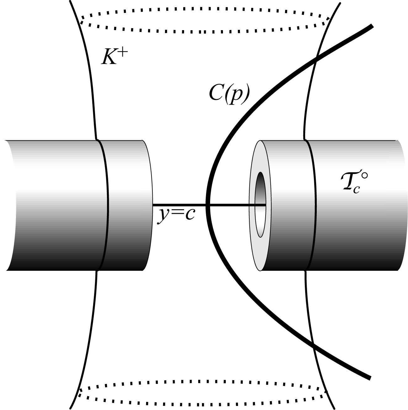
Lemma 4.2.

There exists some $\delta_{T}>0$ and some $\epsilon_{T}>0$ such that if $|a|<\epsilon_{T}$ then:

1. The filled tube $\mathcal{T}^{\boldsymbol{\bullet}}_{c}$ is distance at least $\delta$ from the set ${K}^{\scriptscriptstyle-}_{a}$ for each critical point $c$ of $p(z)$.

2. One has $\overline{\Omega_{c}\times A_{c}}\subset{K}^{\scriptscriptstyle+}_{a}$ for each critical point $c$.

3. For each critical point $c$, $H_{ca}\subset\mathcal{T}^{\hskip 1.0pt\displaystyle{\boldsymbol{\cdot}}}_{c}$ and this is the only component of $\mathscr{C}_{a}$ which intersects $\overline{\mathcal{T}^{\boldsymbol{\bullet}}_{c}}$.

4. The foliations ${\mathcal{F}}^{\scriptscriptstyle+}_{a}$ and ${\mathcal{F}}^{\scriptscriptstyle-}_{a}$ have contact of order two at any point of $H_{ca}$ for any critical point $c$. In particular, $H_{ca}$ is smooth, has multiplicity one, and is everywhere transverse to both ${\mathcal{F}}^{\scriptscriptstyle+}_{a}$ and ${\mathcal{F}}^{\scriptscriptstyle-}_{a}$.

Proof.

1. This is a trivial consequence of the construction of $\mathcal{T}^{\boldsymbol{\bullet}}_{c}$ and Lemma 1.21.

2. This follows from the fact that $\overline{\Omega_{c}\times A_{c}}$ is relatively compact in a basin of attraction of $f_{0}$.

3. We prove first that if $|a|$ is sufficiently small then for each critical point $c$, any component $X$ of $\mathscr{C}_{a}$ which intersects $\overline{\mathcal{T}^{\boldsymbol{\bullet}}_{c}}$ lies in $\mathcal{T}^{\hskip 1.0pt\displaystyle{\boldsymbol{\cdot}}}_{c}$. Hence, for the sake of contradiction, assume that there exists a sequence $a_{i}\to 0$ and a sequence $z_{i}$ such that $z_{i}\in\mathscr{C}_{a_{i}}\cap\overline{\mathcal{T}^{\boldsymbol{\circ}}_{c}}$. It follows from Lemma 2.12 that the sequence $z_{i}$ is bounded. Letting $z_{\infty}$ be any accumulation point of $z_{i}$ then either $z_{\infty}\in{U}^{\scriptscriptstyle+}_{0}$ or $z_{\infty}\in{J}^{\scriptscriptstyle+}_{0}$. One concludes from Lemma 1.12 combined with either Lemma 1.19 in the former case or with Lemma 3.22 in the latter case that $z_{\infty}\in\bigcup\overline{H_{c0}}$. However this is a contradiction since $\overline{\mathcal{T}^{\boldsymbol{\circ}}_{c}}$ is disjoint from each $\overline{H_{c0}}$. Thus $\mathscr{C}_{a}\cap\overline{\mathcal{T}^{\boldsymbol{\circ}}_{c}}=\emptyset$ for $|a|$ sufficiently small.

Now assume $X$ is a component of $\mathscr{C}_{a}$ intersecting $\overline{\mathcal{T}^{\boldsymbol{\bullet}}_{c}}$. Since $X$ is disjoint from $\overline{\Omega_{c}\times A_{c}}$ by part 2 and from $\overline{\mathcal{T}^{\boldsymbol{\circ}}_{c}}$ then it follows easily from the definitions of these sets that $X\subset(\mathbb{C}\setminus\overline{\Omega_{c}})\times B_{c}\subset\mathcal{T}^{\hskip 1.0pt\displaystyle{\boldsymbol{\cdot}}}_{c}$. We will show that $X$ must be $H_{ca}$.

Choose some sequence of points $z_{k}\in X$ such that

$$\lim_{k\to\infty}\mathcal{G}^{\scriptscriptstyle+}_{a}(z_{k})=\sup_{z\in X}\mathcal{G}^{\scriptscriptstyle+}_{a}(z).$$

A straightforward argument by contradiction shows that $z_{k}\to\infty$. By Lemma 2.12, $z_{k}$ converges to the point of the extension of $\mathscr{C}_{a}$ to $\mathbb{P}^{1}\times\mathbb{P}^{1}\times\mathbb{D}_{R}$ with $(u,y,a)$ coordinates $(0,c,a)$. From Theorem 2.13, $X=H_{ca}$.

4. If there is no $\epsilon_{T}$ such as the lemma claims to exist then one can choose a critical point $c$ of $p(x)$ and sequences $a_{k}\to 0$ and $z_{k}\in H_{ca_{k}}$ such that ${\mathcal{L}}^{\scriptscriptstyle+}_{a_{k}}(z_{k})$ and ${\mathcal{L}}^{\scriptscriptstyle-}_{a_{k}}(z_{k})$ have order of contact at least three at $z_{k}$ for each $i$. We can assume without loss of generality that $|z_{k}|\to\infty$ or that $z_{k}$ converges to some point $z_{\infty}\in\overline{\mathcal{T}^{\hskip 1.0pt\displaystyle{\boldsymbol{\cdot}}}_{c}}$.

If $|z_{k}|\to\infty$ then we will need to use the extension of $\mathscr{C}$ to $x=\infty$, hence we change coordinates letting $u=1/x$. Since $z_{k}\in\mathscr{C}_{a_{k}}$ by assumption and the leaves of ${\mathcal{F}}^{\scriptscriptstyle+}_{a_{k}}$ and ${\mathcal{F}}^{\scriptscriptstyle-}_{a_{k}}$ have contact of order at least three at $z_{k}$ then Lemma 2.7 shows that ${\mathcal{F}}^{\scriptscriptstyle+}_{a_{k}}$ and $\mathscr{C}_{a_{k}}$ have intersection multiplicity at least two at $z_{k}$. Since $\mathscr{C}_{a_{k}}$ is defined by $w(u,y,a_{k})$ for $a_{k}$ and $u$ sufficiently small and $y$ bounded then the directional derivative of $w(u,y,a)$ along the leaf of ${\mathcal{F}}^{\scriptscriptstyle+}_{a_{k}}$ through $z_{k}$ is zero by Lemma 2.5. But $\frac{\partial w}{\partial y}(0,c,0)=0$ since this is the directional derivative along the leaf of ${\mathcal{F}}^{\scriptscriptstyle+}_{0}$ by Corollary 2.9. But this contradicts the expression for $w$ about $(0,c,0)$ given in Lemma 2.12.

Having obtained a contradiction if $|z_{k}|\to\infty$, assume $z_{k}\to z_{\infty}=(x_{\infty},y_{\infty})$. By part 1 we know $z_{\infty}\not\in{K}^{\scriptscriptstyle-}_{0}$, so $(x_{\infty},y_{\infty},0)\in\mathfrak{V}_{0,-}$. By Lemma 1.22 we know $z_{\infty}\in\overline{\mathbb{C}^{2}\setminus{K}^{\scriptscriptstyle+}_{0}}$. Hence ${\varphi}_{\scriptscriptstyle-}^{d^{j}}$ is well defined at $(x_{\infty},y_{\infty},0)$ for some integer $j$. Then by either Lemma 3.22 or Lemma 1.19, depending on whether $z_{\infty}\in{J}^{\scriptscriptstyle+}_{0}$ or not, one concludes that one can parameterize plaques of the leaves ${\mathcal{L}}^{\scriptscriptstyle+}_{a_{k}}(z_{k})$ such that they converge to a parameterization of a plaque of the leaf of ${J}^{\scriptscriptstyle+}_{0}$ or ${\mathcal{F}}^{\scriptscriptstyle+}_{0}$ through $z_{\infty}$ (which is a vertical line in either case). Since ${\mathcal{F}}^{\scriptscriptstyle+}_{a_{k}}$ and ${\mathcal{F}}^{\scriptscriptstyle-}_{a_{k}}$ have contact of order at least three at $z_{k}$ for each $k$ then by Lemma 2.5 the directional derivative of ${\varphi}_{a_{k},\scriptscriptstyle-}^{d^{j}}$ along the leaf ${\mathcal{L}}^{\scriptscriptstyle+}_{a_{k}+}(z_{k})$ is zero. But by continuity of ${\varphi}_{\scriptscriptstyle-}^{d^{j}}$ it follows that the directional derivative of ${\varphi}_{0,\scriptscriptstyle-}^{d^{j}}$ in the $y$ direction is zero. This contradicts the expression for ${\varphi}_{0,\scriptscriptstyle-}^{d^{j}}$ given in Lemma 1.12. Hence we conclude that there is no such sequence $a_{k}$ and $z_{k}$ and so ${\mathcal{F}}^{\scriptscriptstyle-}_{a}$ and ${\mathcal{F}}^{\scriptscriptstyle+}_{a}$ have contact of order two at every point of $H_{ca}$ whenever $|a|$ is sufficiently small.

The rest of the Lemma is an immediate consequence of Corollary 2.8. ∎

Lemma 4.3.

If $|a|<\epsilon_{T}$ then the map $\mathcal{G}^{\scriptscriptstyle+}_{a}{\big{\arrowvert}_{H_{ca}}}\colon H_{ca}\to(\frac{1}{d-1}\log|a|,\infty)$ is proper.

Proof.

This is easy to prove using parts 1 and 3 of Lemma 4.2. ∎

The following is a standard fact:

Lemma 4.4.

If $M$ is a Riemann surface and if $g$ is harmonic on $M$ then

• The zeros of $\nabla g$ are discrete

• The zeros of $\nabla g$ correspond to critical points of a holomorphic $h$ such that $g=\operatorname{Re}h$ and the index of the zero is equal the negative of the order of the critical point.

Theorem 4.5.

If $|a|<\epsilon_{T}$ then $H_{ca}$ is a punctured disk and the map ${\varphi}_{a,\scriptscriptstyle+}$ extends holomorphically from from $H_{ca}\cap V_{+}$ to a biholomorphism ${\varphi}_{a,\scriptscriptstyle+}\colon H_{ca}\to\mathbb{C}\setminus\overline{\mathbb{D}}$.

Proof.

Using Lemma 4.4 and part 4 of Lemma 4.2 we can conclude that $\mathcal{G}^{\scriptscriptstyle+}_{a}$ has no critical points on $H_{ca}$. Moreover, by Lemma 4.3, $\mathcal{G}^{\scriptscriptstyle+}_{a}$ is proper. By Theorem 2.13, Corollary 1.16 and the definition of $\mathcal{G}^{\scriptscriptstyle+}_{a}$ it follows that that the fibers of $\mathcal{G}^{\scriptscriptstyle+}_{a}{\big{\arrowvert}_{H_{ca}}}$ about the point $(\infty,c)\in H_{ca}$ are topological circles and, by Morse theory, $H_{ca}$ is a topological annulus. Since $H_{ca}$ contains a punctured disk about $(\infty,c)$ then $H_{ca}$ is either $\mathbb{D}^{*}$ or $\mathbb{C}^{*}$.

The function ${\varphi}_{a,\scriptscriptstyle+}\circ f_{a}^{\circ{k}}\colon H_{ca}\to\mathbb{C}\setminus\overline{\mathbb{D}}$ induces the map $j\mapsto d^{k}\cdot j$ on $\pi_{1}(H_{ca})\to\pi_{1}(\mathbb{C}\setminus\overline{\mathbb{D}})$ by Corollary 1.16, Theorem 2.13 and the recursion relation for ${\varphi}_{a,\scriptscriptstyle+}$. It follows that ${\varphi}_{a,\scriptscriptstyle+}\circ f_{a}^{\circ{k}}$ has a holomorphic $d^{k\text{th}}$ root which is equal to ${\varphi}_{a,\scriptscriptstyle+}$ on $H_{ca}\cap V_{+}$. It then follows that ${\varphi}_{a,\scriptscriptstyle+}$ has a holomorphic extension to all of $H_{ca}$. What is more, ${\varphi}_{a,\scriptscriptstyle+}$ is proper since $\mathcal{G}^{\scriptscriptstyle+}_{a}$ is. By considering ${\varphi}_{a,\scriptscriptstyle+}$ about $(\infty,c)$ it follows easily that ${\varphi}_{a,\scriptscriptstyle+}{\big{\arrowvert}_{H_{ca}}}\colon H_{ca}\to\mathbb{C}\setminus\overline{\mathbb{D}}$ has degree one and is therefore a biholomorphism. ∎

Given $a,b$ with $|a|<\epsilon_{T}$ and $|b|<\epsilon_{T}$ we define a biholomorphism $\tau_{ab}\colon H_{ca}\to H_{cb}$ by $\tau_{ab}=\biggl{(}{\varphi}_{b,\scriptscriptstyle+}{\big{\arrowvert}_{H_{cb}}}\biggr{)}^{-1}\circ{\varphi}_{a,\scriptscriptstyle+}$. Then ${\varphi}_{a,\scriptscriptstyle+}\circ\tau_{ab}={\varphi}_{b,\scriptscriptstyle+}$.

Proposition 4.6.

The maps $\tau_{ab}\colon H_{ca}\to H_{cb}$ vary holomorphically in $a$ and $b$.

Proof.

The precise meaning of this is that if one defines $\mathscr{H}_{c}\subset\mathscr{C}$ to be $\{(x,y,a)|(x,y)\in H_{ca},a\in\mathbb{D}_{\epsilon_{T}}\}$ then from Lemma 2.12 and part 3 of Lemma 4.2 it is clear that $\mathscr{H}_{c}$ is a component of $\mathscr{C}\cap(\mathbb{C}^{2}\times\mathbb{D}_{\epsilon_{T}})$ and this proposition states that the map $\tilde{\tau}\colon\mathscr{H}_{c}\times\mathbb{D}_{\epsilon_{T}}\to\mathscr{H}_{c}$ given by $\tilde{\tau}(x,y,a,b)\equiv\tau_{a,b}(x,y)$ is holomorphic.

The proof is elementary since from our original construction the function ${\varphi}_{a,\scriptscriptstyle+}(x,y)\colon V_{+}\times\mathbb{D}_{R}\to\mathbb{C}$ is holomorphic in $x$, $y$ and $a$. It was shown in the proof of Theorem 4.5 that ${\varphi}_{a,\scriptscriptstyle+}\circ f^{\circ{k}}{\big{\arrowvert}_{H_{ca}}}$ has a $d^{k\text{th}}$ root which agrees with ${\varphi}_{a,\scriptscriptstyle+}$ when $|a|<\epsilon_{T}$ and this root gives the extension of ${\varphi}_{a,\scriptscriptstyle+}$ to $f^{-k}(V_{+})\cap H_{ca}$. It follows that ${\varphi}_{a,\scriptscriptstyle+}\circ f_{a}^{k}(x,y)\colon\mathscr{H}_{c}\cap\{(x,y,a)|f_{a}^{\circ{k}}(x,y)\in V_{+},a\in\mathbb{D}_{\epsilon_{T}}\}\to\mathbb{C}$ has a $d^{k\text{th}}$ root which agrees with ${\varphi}_{a,\scriptscriptstyle+}(x,y)$ on $\mathscr{H}_{c}\cap(V_{+}\times\mathbb{D}_{\epsilon_{T}})$. Consequently the extension ${\varphi}_{a,\scriptscriptstyle+}(x,y)\colon\mathscr{H}_{c}\to\mathbb{C}\setminus\overline{\mathbb{D}}$ is holomorphic in $x$, $y$ and $a$. It is easy to see that the map $\widetilde{{\varphi}_{a,\scriptscriptstyle+}}\equiv\bigl{(}{\varphi}_{a,\scriptscriptstyle+}(x,y),a\bigr{)}\colon\mathscr{H}_{c}\to(\mathbb{C}\setminus\overline{\mathbb{D}})\times\mathbb{D}_{\epsilon_{T}}$ is a biholomorphism. It follows that $\tilde{\tau}_{ab}$ is holomorphic in $a$ and $b$ from the easily verified relationship $\widetilde{{\varphi}_{b,\scriptscriptstyle+}}\circ\tilde{\tau}_{ab}=\widetilde{{\varphi}_{a,\scriptscriptstyle+}}$. ∎

4.2 Classification of the Critical Components.

Since our strategy has been to consider the degenerate map $f_{0}$ and then to consider $\mathscr{C}_{a}$ as a deformation of $\mathscr{C}_{0}$, we need to ensure that we have accounted for every component of $\mathscr{C}_{a}$. It is plausible that $\mathscr{C}_{a}$ has a component that “escapes to infinity” as $a\to 0$, and thus this component would be invisible to us in $\mathscr{C}_{0}$. We will start by showing that any component of $\mathscr{C}_{a}$ meets either ${J}^{\scriptscriptstyle-}_{a}$ or ${J}^{\scriptscriptstyle+}_{a}$. We will be able to use this to show that any component of $\mathscr{C}_{a}$ is an iterate of a component of the form $H_{ca}$, and thus we have accounted for every component of $\mathscr{C}_{a}$ by accounting for the components $H_{ca}$ and their iterates.

Lemma 4.7.

If $W_{a}$ is some component of $\mathscr{C}_{a}$ then $\partial W_{a}$ contains a point in either ${J}^{\scriptscriptstyle+}_{a}$ or ${J}^{\scriptscriptstyle-}_{a}$.

Proof.

Consider the positive plurisubharmonic function $\mathfrak{g}(x,y,a)\equiv\mathcal{G}^{\scriptscriptstyle+}_{a}(x,y)+\mathcal{G}^{\scriptscriptstyle-}_{a}(x,y)-\dfrac{1}{d-1}\log|a|$ on $\tilde{U}^{+}\cap\tilde{U}^{-}$. It is easy to show that if $z_{n}$ is a sequence of points of $W_{a}$ such that $\lim_{n\to\infty}\mathfrak{g}(z_{n})=\inf_{z\in W_{a}}\mathfrak{g}(z)$ then $z_{n}$ has an accumulation point in ${J}^{\scriptscriptstyle+}_{a}\cup{J}^{\scriptscriptstyle-}_{a}$. ∎

We will need specific local stable manifolds about the points of $J_{a}$. We know that if $|a|$ is sufficiently small then given $\underline{z}=(\dotsb,z_{-2},z_{-1},z_{0})\in\hat{J}(p)$ there is an associated neighborhood $B_{z_{0}}=V_{0}\times U_{z_{0}}$ of $\pi_{a}(\underline{z})$ and the local stable manifold in $B_{z_{0}}$ is the graph of a holomorphic function from $V_{0}\to U_{z_{0}}$.

We recall that in Lemma 3.8 it was shown that $(u,v)$ coordinates are defined on an open set $V^{\prime}$ which contains each of the sets $B_{z}$ and that $(u,v)$ coordinates provide a biholomorphic isomorphism of $V^{\prime}$ onto $U^{\prime}\times\mathbb{D}_{\boldsymbol{\delta}}$. Also, since $v(x,y)=p(y)-x$ then $v$ is defined on all of $\mathbb{C}^{2}$, not just on $V^{\prime}$.

Definition 4.8.

We now fix some positive $r<1$ such that each of the filled tubes $\mathcal{T}^{\boldsymbol{\bullet}}_{c}$ is a finite distance from the set $\{(x,y)\in\mathbb{C}^{2}\big{\arrowvert}\ |v(x,y)|\leq r\boldsymbol{\delta}\}$.

Proof that such an $r$ exists..

Each of the filled tubes lies a finite distance from $C(p)$ by construction. We let $s$ be half the minimal distance between $C(p)$ and the nearest tube. Since $\bigl{(}x-v(x,y),y\bigr{)}\in C(p)$ for all $(x,y)\in\mathbb{C}^{2}$ then the set $\{(x,y)\big{\arrowvert}\ |v(x,y)|\leq s\}$ is comprised of points no further than $s$ from $C(p)$. Thus $r=s/\boldsymbol{\delta}$ will do. ∎

Lemma 4.9.

Given $\epsilon>0$ there exists $\delta_{r}(\epsilon)>0$ such that if $|a|<\delta_{r}(\epsilon)$ and if $(x,y)\in V^{\prime}\subset\mathbb{C}^{2}$ then

• $|v(x,y)|\leq r\boldsymbol{\delta}$ implies that $\mathcal{G}^{\scriptscriptstyle-}_{a}(x,y)<\dfrac{1}{d}\log|r\boldsymbol{\delta}|+\epsilon$

• $|v(x,y)|\geq r\boldsymbol{\delta}$ implies that $\dfrac{1}{d}\log|r\boldsymbol{\delta}|-\epsilon<\mathcal{G}^{\scriptscriptstyle-}_{a}(x,y)$

Proof.

This is an easy consequence of Theorem 1.24. ∎

Lemma 4.10.

There exists $\epsilon_{S}>0$ such that if $|a|<\epsilon_{S}$ and $z\in J(p)$ then the gradient of the restriction of $\mathcal{G}^{\scriptscriptstyle-}_{a}$ to the local stable manifold $\check{g}_{z+}(\mathbb{D}_{\boldsymbol{\delta}},a)$ is defined and nonzero on the curve $\check{g}_{z+}(S_{r\boldsymbol{\delta}},a)$.

Proof.

First we recall that $\mathcal{G}^{\scriptscriptstyle-}_{a}-{\dfrac{1}{d-1}}\log|a|$ is pluriharmonic, and is therefore smooth, away from its zero set. From Lemma 4.9 we conclude that as long as $|a|<\delta_{r}(\epsilon)$ and $|a|<\bigl{(}(r\boldsymbol{\delta})^{1/d}e^{-\epsilon}\bigr{)}^{d-1}$ then if $(x,y)\in\check{g}_{z+}(S_{r\boldsymbol{\delta}},a)$ then $(x,y)\in B_{z}\in V^{\prime}$ and $|v(x,y)|=r\boldsymbol{\delta}$ so

$$\mathcal{G}^{\scriptscriptstyle-}_{a}(x,y)-{\dfrac{1}{d-1}}\log|a|>{\dfrac{1}{d}}\log|r\boldsymbol{\delta}|-\epsilon-{\dfrac{1}{d-1}}\log|a|>0.$$

Thus $\mathcal{G}^{\scriptscriptstyle-}_{a}$ is smooth at such points.

Assume that no such $\epsilon_{S}$ existed. Then there exists a sequence $a_{i}\to 0$ and a sequence of points $z_{i}\in J(p)$ and a sequence of points $w_{i}\in U_{z_{i}}\times S_{r\boldsymbol{\delta}}\subset B_{z_{i}}$ such that for each $i$ the restriction of $\mathcal{G}^{\scriptscriptstyle-}_{a_{i}}$ to the stable manifold $\check{g}_{z_{i}+}(\mathbb{D}_{\boldsymbol{\delta}},a)\subset B_{z_{i}}$ has gradient zero at the point $\check{g}_{z_{i}+}(w_{i},a_{i})$. Then by compactness we can replace our sequence with a subsequence if necessary such that both $z_{i}$ converges to some point $z_{\infty}\in J(p)$ and $w_{i}$ converges to some point $w_{\infty}\in V^{\prime}$.

Then by Lemma 3.9 and Lemma 3.18 we see that $\check{g}_{z_{i}+}(w_{i},a_{i})\to\check{g}_{z_{\infty}+}(w_{\infty},0)$ and $w_{\infty}\in U_{z_{\infty}}\times S_{r\boldsymbol{\delta}}\subset V^{\prime}$ and the gradient of the restriction of $\mathcal{G}^{\scriptscriptstyle-}_{0}$ to the stable manifold in $B_{z_{\infty}}$ is zero at the point $\check{g}_{z_{\infty}+}(w_{\infty},0)$ on the curve $\check{g}_{z_{\infty}+}(S_{r\boldsymbol{\delta}},0)$. Since the sequence $\mathcal{G}^{\scriptscriptstyle-}_{a_{k}}\bigl{(}\check{g}_{z_{k}+}(\cdot,a_{k})\bigr{)}$ converges locally uniformly to $\mathcal{G}^{\scriptscriptstyle-}_{0}\bigl{(}\check{g}_{z_{\infty}+}(\cdot,0)\bigr{)}$ by Lemma 3.18, so derivatives of $\check{g}_{z_{k}+}(\cdot,a_{k})$ converge locally uniformly to the derivatives of $\check{g}_{z_{\infty}+}(\cdot,0)$, then because $\mathcal{G}^{\scriptscriptstyle-}_{a}$ is smooth on a neighborhood of the image of $\check{g}_{z_{\infty}+}(S_{r\boldsymbol{\delta}},0)$ then the gradient of $\mathcal{G}^{\scriptscriptstyle-}_{a_{k}}$ projected to the tangent space of $\Delta_{z_{k},a_{k}}$ at $\check{g}_{z_{k}+}(w_{k},a_{k})$ converges to the gradient of $\mathcal{G}^{\scriptscriptstyle-}_{0}$ projected to the tangent space of $\Delta_{z_{k},a_{k}}$ at $\check{g}_{z_{k}+}(w_{\infty},0)$. This is a contradiction since the gradient of the restriction of $\mathcal{G}^{\scriptscriptstyle-}_{0}={\dfrac{1}{d}}\log|v|$ to a vertical line does not vanish on the curve $|v|=r\boldsymbol{\delta}$. ∎

Lemma 4.11.

The index of the gradient of the restriction of $\mathcal{G}^{\scriptscriptstyle-}_{a}$ to $\check{g}_{z+}(\mathbb{D}_{\boldsymbol{\delta}})$ around the curve $\check{g}_{z+}(S_{r\boldsymbol{\delta}})$ is one for all $|a|<\epsilon_{S}$.

Proof.

The lemma is easily seen to be true for $a=0$ since then $\check{g}_{z+}(S_{r\boldsymbol{\delta}})$ is a loop around a single singularity of $\frac{1}{d}\log|p(y)-x|$. By Lemma 4.10, the index can not change for $|a|<\epsilon_{S}$. ∎

Lemma 4.12.

If $a$ is sufficiently small then for any $z\in J(p)$ and for any $w\in p^{-1}(z)$ one has $f_{a}\bigl{(}\Delta_{w,a}(r)\bigr{)}\Subset\Delta_{z,a}(r)$. Also $f_{a}\bigl{(}\Delta_{w_{1},a}(r)\bigr{)}\cap f_{a}\bigl{(}\Delta_{w_{1},a}(r)\bigr{)}=\emptyset$ for $w_{1}$ and $w_{2}$ distinct points of $p^{-1}(z)$.

Proof.

Using Lemma 4.9 it follows that if $(x,y)\in\overline{\Delta_{w,a}(r)}$ and $f_{a}(x,y)\in\overline{\Delta_{w,a}\setminus\Delta_{w,a}(r)}$ then $|a|\geq{\dfrac{(r\boldsymbol{\delta})^{1-1/d}}{\epsilon^{d+1}}}$. The second statement is an immediate consequence of Lemma 3.17. ∎

Lemma 4.13.

There exists $M>0$ such that given $\epsilon>0$ then for $|a|<\epsilon/M$ one has $|v\bigl{(}f_{a}(x,y)\bigr{)}|<\epsilon$ for each $(x,y)\in\mathcal{T}^{\boldsymbol{\bullet}}_{c}$ and for each critical point $c$ of $p(x)$.

Proof.

One has $|v\bigl{(}f_{a}(x,y)\bigr{)}|=|v\bigl{(}p(x)-ay,x\bigr{)}|=|ay|$. Choosing $M>0$ such for each critical point $c$ of $p(x)$ one has $\mathcal{T}^{\boldsymbol{\bullet}}_{c}\subset(\mathbb{D}_{M}\times\mathbb{C})$ one concludes that taking $|a|<{\dfrac{\epsilon}{M}}$ is sufficient. ∎

We will let $V^{\prime}_{r}\equiv\{(x,y)\in V^{\prime}\big{\arrowvert}\ |v(x,y)|<r\}$.

Corollary 4.14.

If $a$ is sufficiently small then for any $z\in J(p)$ the set $\overline{\Delta_{z,a}(r)}\setminus\bigcup_{w\in p^{-1}(z)}f_{a}\bigl{(}\Delta_{w,a}(r)\bigr{)}$ contains no points of $J_{a}$.

Proof.

If $a$ is sufficiently small then $J_{a}\subset V^{\prime}_{r}$ and $\pi_{a}$ is defined. Since $J_{a}\subset V^{\prime}_{r}$ then given any $\underline{z}=(\dotsb,z_{-2},z_{-1},z_{0})\in\hat{J}(p)$ then $\pi_{a}(\underline{z})\in\Delta_{z,a}(r)$. From Lemma 3.17 we know that a point in $J_{a}$ can lie in $\Delta_{z,a}$ iff the corresponding history in $\hat{J}(p)$ ends with the point $z$. Then the result is easy since the set removed from $\overline{\Delta_{z,a}(r)}$ contains all points in $J_{a}$ corresponding to histories in $\hat{J}(p)$ which could end with $z_{0}$. ∎

Corollary 4.15.

There exists $\epsilon>0$ such that if $|a|<\epsilon$ then the index of the vector field $\nabla(\mathcal{G}^{\scriptscriptstyle-}_{a}{\big{\arrowvert}_{\Delta_{z,a}}})$ around the boundary of $\overline{\Delta_{z,a}(r)}\setminus\bigcup_{w\in p^{-1}(z)}f_{a}\bigl{(}\Delta_{w,a}(r)\bigr{)}$ is $1-d$.

Proof.

We note from Corollary 4.14 that $\mathcal{G}^{\scriptscriptstyle-}_{a}>0$ on $\overline{\Delta_{z,a}(r)}\setminus\bigcup_{w\in p^{-1}(z)}f_{a}\bigl{(}\Delta_{w,a}(r)\bigr{)}$ and so it will be pluriharmonic on a neighborhood of $\overline{\Delta_{z,a}(r)}\setminus\bigcup_{w\in p^{-1}(z)}f_{a}\bigl{(}\Delta_{w,a}(r)\bigr{)}$. Thus $\nabla(\mathcal{G}^{\scriptscriptstyle-}_{a}{\big{\arrowvert}_{\Delta_{z,a}}})$ will have only finitely many zeros in $\overline{\Delta_{z,a}(r)}\setminus\bigcup_{w\in p^{-1}(z)}f_{a}\bigl{(}\Delta_{w,a}(r)\bigr{)}$. By Lemma 4.10 we know none of these zeros lie on the boundary.

The result then follows as long as $\epsilon$ is sufficiently small as a consequence of Lemma 4.11 and Lemma 4.12. ∎

We recall [BS99] Proposition 2.7, noting that the hypothesis is satisfied for all $a$ under consideration since $f_{a}$ is hyperbolic when the crossed mapping construction of [HOV95] applies, and there is a continuous surjection from $\hat{J}(p)$ to $J_{a}$, and hence $J_{a}$ is connected. Since $J_{a}$ is connected and $|a|<1$ then by Theorem 0.2 of [BS98b] it follows that $f_{a}$ is unstably connected.

Proposition 4.16.

If $f_{a}$ is hyperbolic and unstably connected, then the union of ${\mathcal{F}}^{\scriptscriptstyle+}_{a}$ and the stable lamination of $f_{a}{\big{\arrowvert}_{{J_{a}}}}$ form a lamination of the space ${U}^{\scriptscriptstyle+}_{a}\cup{J}^{\scriptscriptstyle+}_{a}$.

Observation 4.17.

For the maps we are studying, the union of ${\mathcal{F}}^{\scriptscriptstyle-}_{a}$ and the unstable lamination of $f_{a}{\big{\arrowvert}_{{J_{a}}}}$ do not form a lamination of the space ${U}^{\scriptscriptstyle-}_{a}\cup{J}^{\scriptscriptstyle-}_{a}$. This is because critical points on the local stable manifolds are tangencies between the stable foliation and ${\mathcal{F}}^{\scriptscriptstyle-}_{a}$. Taking forward images of these tangencies gives accumulations of such tangencies near $J_{a}$. But ${J}^{\scriptscriptstyle-}_{a}$ is transverse to ${J}^{\scriptscriptstyle+}_{a}$ everywhere since the map is hyperbolic, so the unstable foliation and ${\mathcal{F}}^{\scriptscriptstyle-}_{a}$ can’t be part of the same foliation.

We let $K^{\circ}(p)$ denote the interior of the filled Julia set of $p(x)$.

Proposition 4.18.

For all sufficiently small nonzero $a$, given any $z\in J(p)$ then the only points of $\overline{\mathscr{C}_{a}}$ which lie in $f_{a}^{-1}\bigl{(}\Delta_{z,a}(r)\bigr{)}\setminus\bigcup_{w\in p^{-1}(z)}\Delta_{w,a}(r)$ are the points $\tau_{0a}(z,c)\in\tau_{0a}(\partial H_{c0})=\partial H_{ca}$ where $c$ is a critical point of $p(z)$.

Additionally, when $a$ and $b$ are sufficiently small the biholomorphism $\tau_{ab}\colon H_{ca}\to H_{cb}$ defined in Section 4.1 extends naturally to a homeomorphism between $\overline{H_{ca}}$ and $\overline{H_{cb}}$. Since $\overline{H_{c0}}$ can be naturally identified with $\mathbb{C}\setminus K^{\circ}(p)$ then the same is true for $\overline{H_{ca}}$.

Proof.

We choose $\epsilon$ small enough that:

1. $\epsilon\leq\epsilon_{T}$, so Lemma 4.2 holds for $|a|<\epsilon$,

2. $J_{a}\subset V^{\prime}$ when $|a|<\epsilon$, which we can do by Lemma 3.19,

3. $\epsilon<r\boldsymbol{\delta}/M$ for the value $M$ in Lemma 4.13,

4. Lemma 4.12, Corollary 4.14 and Corollary 4.15 all hold for $|a|<\epsilon$.

We will show the result holds for $|a|<\epsilon$.

Given a critical point $c$ of $p(x)$, we let $\tilde{H}_{c}=\{(x,y,a)|(x,y)\in H_{ca},a\in\mathbb{D}_{\epsilon}\}$. Now given an arbitrary point $z\in\mathbb{C}\setminus K(p)$ we define the map $h_{cz}\colon\mathbb{D}_{\epsilon}\to\tilde{H}_{c}\subset\mathbb{C}^{2}\times\mathbb{D}_{\epsilon}$ by $h_{cz}(a)\equiv\bigl{(}\tau_{0a}(z,c),a\bigr{)}\in\tilde{H}_{c}$. It follows from Proposition 4.6 that $h_{cz}$ is holomorphic. One easily confirms that ${\varphi}_{a,\scriptscriptstyle+}\bigl{(}h_{cz}(a)\bigr{)}={\varphi}_{0,\scriptscriptstyle+}(z,c)$ which is independent of $a$. It follows that

$$\mathcal{G}^{\scriptscriptstyle+}\bigl{(}h_{cz}(a)\bigr{)}\equiv\mathcal{G}^{\scriptscriptstyle+}_{0}(z,c)\text{\ for\ }a\in\mathbb{D}_{\epsilon}.$$ (4.1)

We also note that by Corollary 1.15 there is some radius $R^{\prime}$ such that for each critical point $c$ of $p(x)$, if $|x|\geq R^{\prime}$, $(x,y)\in\overline{\mathcal{T}^{\boldsymbol{\bullet}}_{c}}$ and $|a|<\epsilon$ then $\mathcal{G}^{\scriptscriptstyle+}_{a}(x,y)\geq 1$. Hence if $(x,y)\in H_{ca}$ and $\mathcal{G}^{\scriptscriptstyle+}_{a}(x,y)<1$ then $(x,y)\in W_{c}\equiv\Bigl{(}\overline{\mathcal{T}^{\boldsymbol{\bullet}}_{c}}\cap(\mathbb{D}_{R^{\prime}}\times\mathbb{C})\Bigr{)}\times\mathbb{D}_{\epsilon}$. The set $W_{c}$ is clearly a bounded set in $\mathbb{C}^{3}$ since the set $\mathbb{D}_{R^{\prime}}\times\mathbb{C}$ has bounded $x$ coordinates and the set $\overline{\mathcal{T}^{\boldsymbol{\bullet}}_{c}}$ has bounded $y$ coordinates.

We let $Y=\{z\in\mathbb{C}\setminus K(p)\ |\ \mathcal{G}^{\scriptscriptstyle+}_{0}(z,c)<1\}$. If $z\in Y$ then $h_{cz}(a)$ lands in the set $W_{c}$ since $\mathcal{G}^{\scriptscriptstyle+}\bigl{(}h_{cz}(a)\bigr{)}=\mathcal{G}^{\scriptscriptstyle+}_{0}(z,c)<1$ for all $a\in\mathbb{D}_{\epsilon}$. Since $W_{c}$ is bounded it follows that $\{h_{cz}|z\in Y\}$ is a normal family of maps from $\mathbb{D}_{\epsilon}$ into $\mathbb{C}^{3}$. The condition that $\mathcal{G}^{\scriptscriptstyle+}_{0}(z,c)<1$ is the same as $\log|b_{p}(z)|<1$ so $J(p)\times\{c\}\times\{0\}\subset\overline{Y}$.

To complete the proof of Proposition 4.18 we need two lemmas.

Lemma 4.19.

Assume $z_{k}$ is a sequence of points of $\mathbb{C}\setminus K(p)$ converging to a point $z_{\infty}\in J(p)$. Then, for each critical point $c$, the limit $g$ of any convergent subsequence of $h_{cz_{k}}$ satisfies $g(a)\in f_{a}^{-1}\bigl{(}\Delta_{z_{\infty},a}(r)\bigr{)}$ for all $a\in\mathbb{D}_{\epsilon}$.

Proof of Lemma 4.19.

We will show that $f_{a}\bigl{(}g(a)\bigr{)}\in\Delta_{z_{\infty},a}(r)$ for all $a\in\mathbb{D}_{\epsilon}$. By Lemma 4.13, since $|a|<\epsilon<r\boldsymbol{\delta}/M$, then $|v\bigl{(}f_{a}(\mathcal{T}^{\boldsymbol{\bullet}}_{c})\bigr{)}|<r\boldsymbol{\delta}$. Recall that $V^{\prime}_{r}=\{(x,y)\in V^{\prime}\big{\arrowvert}\ |v|<r\boldsymbol{\delta}\}=U^{\prime}\times\mathbb{D}_{r\boldsymbol{\delta}}$. Now $\tilde{\Delta}_{z_{\infty},a}(r)\equiv\{(x,y,a)|(x,y)\in\Delta_{z_{\infty},a}(r),a\in\mathbb{D}_{\epsilon}\}$ is defined in $V^{\prime}_{r}\times\mathbb{D}_{\epsilon}$ as the graph of $g_{z_{\infty}+}\colon\mathbb{D}_{r\boldsymbol{\delta}}\times\mathbb{D}_{\epsilon}\to U^{\prime}$. Thus $v-g_{z_{\infty}+}(u,a)$ is a holomorphic defining function for $\tilde{\Delta}_{z_{\infty},a}(r)\subset V^{\prime}_{r}\times\mathbb{D}_{\epsilon}$. Since $\mathcal{G}^{\scriptscriptstyle+}_{a}\bigl{(}h_{cz_{k}}(a)\bigr{)}>0$ for each $k$, then $\bigl{(}v-g_{z_{\infty}}(u,a)\bigr{)}\circ\tilde{f}\circ h_{cz_{k}}$ is nonvanishing on $\mathbb{D}_{\epsilon}$ for each $k$ whenever it is defined, i.e. whenever $h_{cz_{k}}\in V^{\prime}_{r}\times\mathbb{D}_{\epsilon}$. If $g$ is the limit of any convergent subsequence, then $\bigl{(}v-g_{z_{\infty}+}(u,a)\bigr{)}\circ f_{0}\circ g(0)=0$. Since $g$ maps $\mathbb{D}_{\epsilon}$ into $\{(x,y)|\ |v(x,y)|<r\boldsymbol{\delta}\}$ it can be shown that the set on which $\bigl{(}v-g_{z_{\infty}+}(u,a)\bigr{)}\circ\tilde{f}\circ g$ vanishes is both open and closed in $\mathbb{D}_{\epsilon}$, so it is all of $\mathbb{D}_{\epsilon}$. Thus $g(a)\in f_{a}^{-1}\bigl{(}\Delta_{z_{\infty},a}(r)\bigr{)}$ for all $a\in\mathbb{D}_{\epsilon}$. ∎

Lemma 4.20.

Assume $z_{k}$ is a sequence of points of $\mathbb{C}\setminus K(p)$ converging to a point $z_{\infty}\in J(p)$. Then the limit $g$ of any convergent subsequence of $h_{cz_{k}}$ is disjoint from $\Delta_{w,a}(r)$ for each $w\in p^{-1}(z_{\infty})$ for all $a\in\mathbb{D}_{\epsilon}$ and for each critical point $c$.

Proof of Lemma 4.20..

Each $g(a)\in\mathcal{T}^{\boldsymbol{\bullet}}_{c}$ lies a positive distance from $|v|<r\boldsymbol{\delta}$ by Definition 4.8. Since $\Delta_{w,a}(r)\subset V^{\prime}_{r}$ this completes the proof. ∎

Now consider an arbitrary critical point $c_{0}$ of $p(z)$. Consider also an arbitrary $a\in\mathbb{D}_{\epsilon}$ and a sequence of points $\{w_{i}\}\in H_{c_{0}a}$ which converge to a point $w_{\infty}\in\overline{H_{c_{0}a}}\cap(J_{a+}\cup J_{a-})$ . Then let $(z_{i},c_{0})=\tau_{a0}(w_{i})\in H_{c_{0}0}$ and consider the sequence of maps $h_{cz_{k}}\colon\mathbb{D}_{\epsilon}\to\mathbb{C}^{3}$ for each critical point $c$.

This is a normal family. Choose some subsequence $h_{cz_{k_{i}}}$ so that $h_{cz_{k_{i}}}$ converges for each critical point $c$. For each critical point $c$ let $g_{c}$ be the limit of this subsequence. By Lemma 4.19, $g_{c}(a)\in f_{a}^{-1}\bigl{(}\Delta_{z_{\infty},a}(r)\bigr{)}$. By Lemma 4.2, $g_{c}(a)\not\in{J}^{\scriptscriptstyle-}_{a}$, so $\mathcal{G}^{\scriptscriptstyle-}_{a}$ is smooth at $g_{c}(a)$. Since $g_{c}(a)$ is a limit of points of $H_{ca_{0}}$ then by Proposition 4.16, ${\mathcal{F}}^{\scriptscriptstyle-}_{a}$ and ${J}^{\scriptscriptstyle+}_{a}$ are tangent at $g_{c}(a)$ and so $g_{c}(a)$ is a point where $\nabla(\mathcal{G}^{\scriptscriptstyle-}_{a}{\big{\arrowvert}_{f_{a}^{-1}\bigl{(}\Delta_{z_{\infty},a}(r)\bigr{)}}})$ has nonzero index.

Now if $a\not=0$ then since there are $d-1$ critical points of $p(x)$ then the set $\{g_{c}(a)|c\text{\ a critical point}\}$ is a set of $d-1$ points of nonzero index in $f_{a}^{-1}\bigl{(}\Delta_{z_{\infty},a}(r)\bigr{)}\setminus\bigcup_{w\in p^{-1}(z_{\infty})}\Delta_{w,a}$.

Since the index of the gradient of the restriction of $\mathcal{G}^{\scriptscriptstyle-}_{a}$ is a vector field in $\Delta_{z_{\infty},a}(r)\setminus\bigcup_{w\in p^{-1}(z_{\infty})}f_{a}\bigl{(}\Delta_{w,a}(r)\bigr{)}$ by Corollary 4.14, and the index around the boundary of this set is $1-d$ by Corollary 4.15, then the same is clearly true for $f_{a}^{-1}\bigl{(}\Delta_{z_{\infty},a}(r)\bigr{)}\setminus\bigcup_{w\in p^{-1}(z_{\infty})}\Delta_{w,a}(r)$. Thus each of the $d-1$ points $g_{c}(a)$ has index $-1$ and $g_{c}(a)$ is the unique point of nonzero index in the intersection of $f_{a}\bigl{(}\Delta_{z_{\infty},a}(r)\bigr{)}\setminus\bigcup_{w\in p^{-1}(z_{\infty})}\Delta_{w,a}(r)$ and the tube $\mathcal{T}^{\boldsymbol{\bullet}}_{c}$. That the same holds for $a=0$ is easy to verify directly.

It follows that given any critical point $c$ of $p(z)$ then any convergent subsequence of $h_{cz_{k}}$ must converge to $g_{c}$. It follows that $h_{cz_{k}}\to g_{c}$. We denote $g_{c}$ by $h_{cz_{\infty}}\colon\mathbb{D}_{\epsilon}\to\mathbb{C}^{3}$. We have thus shown that, given a critical point $c$, if $z_{k}\in\mathbb{C}\setminus K(p)$ converges to $z_{\infty}\in J(p)$ then $h_{cz_{k}}(a)\equiv\bigl{(}\tau_{0a}(z,c),a\bigr{)}\in\tilde{H}_{c}$ converges to a holomorphic function $g_{c}$ such that $g_{c}(a)$ is the unique point of nonzero index in the intersection of $\mathcal{T}^{\boldsymbol{\bullet}}_{c}$ and $f_{a}^{-1}\bigl{(}\Delta_{z_{\infty},a}(r)\bigr{)}\setminus\bigcup_{w\in p^{-1}(z_{\infty})}\Delta_{w,a}(r)$.

We now construct the extension $\tau_{ab}\colon\overline{H_{ca}}\to\overline{H_{cb}}$ by defining $\tau_{ab}(w_{\infty})=h_{cz_{\infty}}(b)$ whenever $w_{\infty}\in\overline{H_{ca}}$ and $z_{\infty}$ is the limit of $\{\tau_{a0}(w_{k})\}$ where $w_{k}\to w_{\infty}$. This is well defined because if $w_{k}\to w_{\infty}$ and $w_{k}^{\prime}\to w_{\infty}$ then $w_{1},w^{\prime}_{1},w_{2},w^{\prime}_{2},\dotsc$ converges to $w_{\infty}$ and by the above, the sequence of maps $h_{c\tau_{a0}(w_{1})},h_{c\tau_{a0}(w_{1}^{\prime})},\dotsc$ converges to a single map $h_{cz_{\infty}}$ for $|a|<\epsilon$. This is also continuous since if $w_{k}\in\overline{H_{ca}}$ and $w_{k}$ converges to $w_{\infty}\in\overline{H_{ca}}$ but $\tau_{ab}(w_{k})\not\to\tau_{ab}(w_{\infty})$ then there exists $\epsilon_{1}>0$ such that there are arbitrarily large values of $k$ with $|\tau_{ab}(w_{k})-\tau_{ab}(w_{\infty})|>\epsilon_{1}$. Then replace each point $w_{k}$ with a point $w_{k}^{\prime}\in H_{ca}$ such that $|w^{\prime}_{k}-w_{k}|<{1}/{2^{k}}$ and $|\tau_{ab}(w^{\prime}_{k})-\tau_{ab}(w_{k})|<\epsilon/2$ (which we can do by the definition of $\tau_{ab}(w_{k})$ if $w_{k}\in\overline{H_{ac}}\setminus H_{ac}$ and we just take $w^{\prime}_{k}=w_{k}$ otherwise). Then $w^{\prime}_{k}$ is a sequence in $H_{ac}$ and $\tau_{ab}(w^{\prime}_{k})$ can not converge to $\tau_{ab}(w_{\infty})$ because there are arbitrarily large $k$ for which $|\tau_{ab}(w^{\prime}_{k})-\tau_{ab}(w_{\infty})|>|\tau_{ab}(w_{k})-\tau_{ab}(w_{\infty})|-|\tau_{ab}(w^{\prime}_{k})-\tau_{ab}(w_{k})|>\epsilon/2$ but $w^{\prime}_{k}\to w_{\infty}$ since $|w^{\prime}_{k}-w_{k}|<1/2^{k}$. But this is a contradiction since $h_{c\tau_{a0}(w^{\prime}_{k})}\to h_{c\tau_{a0}(w_{\infty})}$ by our previous work and $h_{c\tau_{a0}(w^{\prime}_{k})}(a)=w_{k^{\prime}}$ and $h_{c\tau_{a0}(w^{\prime}_{k})}(b)=\tau_{ab}(w^{\prime}_{k})$ by definition. Therefore $\tau_{ab}\colon\overline{H_{ca}}\to\overline{H_{cb}}$ is continuous. Since $\tau_{ba}$ is clearly the inverse of $\tau_{ab}$ then $\tau_{ab}$ is a homeomorphism. This completes the proof of Proposition 4.16. ∎

Theorem 4.21.

For all sufficiently small $a$ every component of the critical locus is an iterate of one of the components $H_{c}$.

Proof.

The components of $H_{ca}$ are the only components of the critical locus if $a=0$, so assume $a\not=0$. If $W$ is a component of $\mathscr{C}_{a}$ then by Lemma 4.7 we know that $\partial W$ contains at least one point $w$ in either ${J}^{\scriptscriptstyle+}_{a}$ or ${J}^{\scriptscriptstyle-}_{a}$. If $w$ lies in ${J}^{\scriptscriptstyle+}_{a}\setminus{J}^{\scriptscriptstyle-}_{a}$ then $w$ lies in the stable manifold of some point of $J_{a}$ so there is some $n^{\prime}$ such that $f_{a}^{\circ{n^{\prime}}}(w)\in\Delta_{z^{\prime},a}(r)$ for some $z^{\prime}\in J(p)$. Take $n$ to be the smallest such $n^{\prime}$ (where $n^{\prime}$ is allowed to be negative) and take $z$ to be the corresponding point of $J(p)$. We know a smallest such $n$ exists since $w\in{J}^{\scriptscriptstyle+}_{a}\setminus{J}^{\scriptscriptstyle-}_{a}$ so $\mathcal{G}^{\scriptscriptstyle-}_{a}(w)-{\dfrac{1}{d-1}}\log|a|>0$ so $\mathcal{G}^{\scriptscriptstyle-}_{a}\bigl{(}f_{a}^{-k}(w)\bigr{)}-{\dfrac{1}{d-1}}\log|a|=d^{n}\cdot\bigl{(}\mathcal{G}^{\scriptscriptstyle-}_{a}(w)-{\dfrac{1}{d-1}}\log|a|\bigr{)}\to\infty$ as $k\to\infty$ but $\mathcal{G}^{\scriptscriptstyle-}_{a}$ is bounded on compact sets (since $V_{0}$ can certainly be assumed to be large enough to contain $V^{\prime}$).

It follows from our choice of $n$ that $f_{a}^{\circ{n}}(w)\in\Delta_{z,a}(r)\setminus\bigcup_{y\in p^{-1}(z)}f_{a}\bigl{(}\Delta_{y,a}(r)\bigr{)}$. But then from Proposition 4.18 and Lemma 4.2 we conclude that $f_{a}^{\circ{n}}(W)$ is an iterate of some $H_{c}$.

On the other hand if $w\in{J}^{\scriptscriptstyle-}_{a}$ then choose a sequence of points $w_{i}\in W$ such that $w_{i}\to w$. Then $\mathcal{G}^{\scriptscriptstyle+}_{a}(w_{i})\to\mathcal{G}^{\scriptscriptstyle+}_{a}(w)=\mathfrak{g}\geq 0$, and $\mathcal{G}^{\scriptscriptstyle-}_{a}(w_{i})-{\dfrac{1}{d-1}}\log|a|\to\mathcal{G}^{\scriptscriptstyle-}_{a}(w)-{\dfrac{1}{d-1}}\log|a|=0$. Then for every $i\geq 1$ choose $n_{i}$ such that $1<\mathcal{G}^{\scriptscriptstyle-}_{a}\bigl{(}f_{a}^{-n_{i}}(w_{i})\bigr{)}-{\dfrac{1}{d-1}}\log|a|\leq d$. By the recursion relation for $\mathcal{G}^{\scriptscriptstyle-}_{a}$ it follows that $n_{i}\to\infty$ as $i\to\infty$. Then $\mathcal{G}^{\scriptscriptstyle+}_{a}\bigl{(}f_{a}^{-n_{i}}(w_{i})\bigr{)}\to 0$ as $i\to\infty$ so the sequence $f_{a}^{-n_{i}}(w_{i})$ is a bounded sequence of points in iterates of $W\subset\mathscr{C}_{a}$ converging to ${J}^{\scriptscriptstyle+}_{a}$. By Proposition 4.18 and Lemma 4.2 the members of any convergent subsequence of $f_{a}^{-n_{i}}(w_{i})$ must lie in an iterate of $H_{c}$ for all large $i$, so $W$ must be an iterate of $H_{c}$. This completes the proof. ∎

Part III Rigidity

5 Holonomy in the Critical Locus.

We will now consider a single map $f=f_{a}$, $a\not=0$ to which Theorem 4.21 applies and for which $|a|<\epsilon_{T}$ (so Lemma 4.2 and Theorem 4.5 apply). Since $a$ is fixed we let $\psi_{+}\equiv{\varphi}_{a,\scriptscriptstyle+}$ and $\psi_{-}\equiv\eta\cdot{\varphi}_{a,\scriptscriptstyle-}\circ f^{-1}$ where $\eta^{d-1}=1/a$ and $\eta$ is fixed. This gives the simpler relations $\psi_{-}\circ f^{-1}=\psi_{-}^{d}$ and $\psi_{+}\circ f=\psi_{+}^{d}$. The function $\psi_{-}$ is well defined and holomorphic on $f(V_{-})$. We will show that $\psi_{-}$ is a biholomorphism from a neighborhood of infinity in $H_{c}$ to a neighborhood of infinity in $\mathbb{C}$. Because $a$ is fixed we will omit it from the notation throughout the rest of this section.

Lemma 5.1.

There is a neighborhood $H_{c}^{\circ}$ of infinity in $H_{c}$ which lies in $f(V_{-})$ and such that $\psi_{-}$ is a biholomorphism from $H_{c}^{\circ}$ to $\mathbb{C}\setminus\overline{\mathbb{D}}_{\mathfrak{r}}$ for some $\mathfrak{r}>1$.

Proof.

First we note that

$$f(V_{-})=\{(x,y)|\ |p(y)-x|>|ay|\ \text{and}\ |p(y)-x|>|a|\alpha\}.$$

Since the $y$ coordinate of points $(x,y)\in H_{c}$ remain bounded as $|x|\to\infty$, it follows that $(x,y)\in H_{c}$ implies $(x,y)\in f(V_{-})$ whenever $|x|$ is sufficiently large. This implies the first assertion.

To show the second result we consider $H_{c}$ to be lying in $\mathbb{C}^{2}\subset\mathbb{P}^{1}\times\mathbb{P}^{1}$. We then know that $H_{c}$ can be completed to become a disk by adding the point $(\infty,c)$ and that its tangent space is given at $(\infty,c)$ by $p^{\prime\prime}(c)\mathbf{d}y+C\mathbf{d}u=0$ where $C$ is some constant and $u={\dfrac{1}{x}}$. From Corollary 1.5 we obtain

$$B^{-1}<\Bigl{\arrowvert}{\dfrac{{\varphi}_{\scriptscriptstyle-}(x,y)}{y}}\Bigr{\arrowvert}<B$$

for $(x,y)\in V_{-}$. Now if $(x,y)\in f(V_{-})$ then $f^{-1}(x,y)=\Bigl{(}y,{\dfrac{p(y)-x}{a}}\Bigr{)}\in V_{-}$ and so we obtain $B^{-1}\Bigl{\arrowvert}{\dfrac{p(y)-x}{a}}\Bigr{\arrowvert}<\arrowvert{\varphi}_{\scriptscriptstyle-}\bigl{(}f^{-1}(x,y)\bigr{)}\arrowvert<B\Bigl{\arrowvert}{\dfrac{p(y)-x}{a}}\Bigr{\arrowvert}$. Since ${\varphi}_{\scriptscriptstyle-}\circ f^{-1}=\psi_{-}/\eta$ this becomes

$$B^{-1}\Bigl{\arrowvert}\eta{\dfrac{p(y)-x}{a}}\Bigr{\arrowvert}<\arrowvert\psi_{-}(x,y)\arrowvert<B\Bigl{\arrowvert}\eta{\dfrac{p(y)-x}{a}}\Bigr{\arrowvert}$$

for $(x,y)\in f(V_{-})$. From Corollary 1.15 we have $B^{-1}|x|<|\psi_{+}(x,y)|<B|x|$ for $(x,y)\in V_{+}$. Dividing one equality by the other gives

$$B^{-2}\Bigl{\arrowvert}\eta{\dfrac{p(y)-x}{ax}}\Bigr{\arrowvert}<\Bigl{\arrowvert}{\dfrac{\psi_{-}(x,y)}{\psi_{+}(x,y)}}\Bigr{\arrowvert}<B^{2}\Bigl{\arrowvert}\eta{\dfrac{p(y)-x}{ax}}\Bigr{\arrowvert}.$$

Since ${\dfrac{p(y)-x}{x}}$ is bounded on $H_{c}$ as $|x|\to\infty$, by the Riemann extension theorem ${\dfrac{\psi_{-}(x,y)}{\psi_{+}(x,y)}}$ is holomorphic and nonzero on a neighborhood of $\infty\in H_{c}$. Hence by shrinking $H_{c}^{\circ}$ if necessary we conclude that $\psi_{-}(x,y)$ is a biholomorphism from the neighborhood $H_{c}^{\circ}$ of $\infty$ onto $\mathbb{C}\setminus\overline{\mathbb{D}_{\mathfrak{r}}}$ for some large $\mathfrak{r}$. ∎

The following is shown in Proposition 6.2 of [HOV95].

Lemma 5.2.

There exists $\mathfrak{R}>1$ such that for any $z\in\mathbb{C}$ with $|z|>\mathfrak{R}$ the fiber of $\psi_{+}$ in $V_{+}$ over $z$ and the fiber of $\psi_{-}$ in $f(V_{-})$ over $z$ are each analytic disks.

Definition 5.3.

Noting that $|\psi_{+}|$ and $|\psi_{-}|$ are well defined on all of ${U}^{\scriptscriptstyle+}$ and ${U}^{\scriptscriptstyle-}$ respectively, we let

$$\mathscr{V}_{+}\equiv\{z\in V_{+}|\ |\psi_{+}(z)|>\mathfrak{R}\}$$

and we let

$$\mathscr{V}_{-}\equiv\{z\in V_{-}|\ |\psi_{-}(z)|>\mathfrak{R}\}.$$

We note that $f(\mathscr{V}_{+})\subset\mathscr{V}_{+}$ and $f^{-1}(\mathscr{V}_{-})\subset\mathscr{V}_{-}$ as follows from the recursion relations for $\psi_{+}$ and $\psi_{-}$.

The following is a consequence of the definitions:

Lemma 5.4.

Two points $z_{1}$ and $z_{2}$ are on the same leaf of ${\mathcal{F}}^{\scriptscriptstyle+}$ iff there exists $n\geq 0$ such that $f^{\circ{n}}(z_{1}),f^{\circ{n}}(z_{2})\in\mathscr{V}_{+}$ and $\psi_{+}\bigl{(}f^{\circ{n}}(z_{1})\bigr{)}=\psi_{+}\bigl{(}f^{\circ{n}}(z_{2})\bigr{)}$. Similarly, two points $z_{1}$ and $z_{2}$ are on the same leaf of ${\mathcal{F}}^{\scriptscriptstyle-}$ iff there exists $n\geq 0$ such that $f^{-n}(z_{1}),f^{-n}(z_{2})\in\mathscr{V}_{-}$ and $\psi_{-}\bigl{(}f^{-n}(z_{1})\bigr{)}=\psi_{-}\bigl{(}f^{-n}(z_{2})\bigr{)}$.

Let $\mathscr{S}\equiv\{\omega\in\mathbb{C}|\omega^{d^{n}}=1\ \text{for some}\ n\geq 0\}\cong\mathbb{Q}_{d}/\mathbb{Z}.$ Given two points $z_{1},z_{2}\in{U}^{\scriptscriptstyle+}$, it is clear that the property ${\dfrac{\psi_{+}(z_{1})}{\psi_{+}(z_{2})}}\in\mathscr{S}$ is independent of the branches of $\psi_{+}$ used. Similarly for the property ${\dfrac{\psi_{-}(z_{1})}{\psi_{-}(z_{2})}}\in\mathscr{S}$, $z_{1},z_{2}\in{U}^{\scriptscriptstyle-}$.

Lemma 5.5.

Two points $z_{1},z_{2}\in{U}^{\scriptscriptstyle+}$ are on the same leaf of ${\mathcal{F}}^{\scriptscriptstyle+}$ iff ${\dfrac{\psi_{+}(z_{1})}{\psi_{+}(z_{2})}}\in\mathscr{S}$. Similarly, two points $z_{1},z_{2}\in{U}^{\scriptscriptstyle-}$ are on the same leaf of ${\mathcal{F}}^{\scriptscriptstyle-}$ iff ${\dfrac{\psi_{-}(z_{1})}{\psi_{-}(z_{2})}}\in\mathscr{S}$.

Proof.

If $z_{1}$ and $z_{2}$ lie in $\mathscr{V}_{+}$ the first assertion follows from Lemmas 5.2 and 5.4 and the recursion relationship for $\psi_{+}$. Otherwise, choosing $k$ such that $f^{\circ{k}}(z_{1}),f^{\circ{k}}(z_{2})\in\mathscr{V}_{+}$ gives the first assertion. The second is analogous. ∎

We will want to consider the holonomy maps of $H_{c}$ determined by the foliations ${\mathcal{F}}^{\scriptscriptstyle+}$ and ${\mathcal{F}}^{\scriptscriptstyle-}$. By Theorem 4.5, $H_{c}$ can be identified with $\mathbb{C}\setminus\overline{\mathbb{D}}$ using $\psi_{+}$.

Assume that $z_{1}$ and $z_{2}$ are points of $H_{c}$ for some critical point $c$ of $p(z)$ and that $z_{1}$ and $z_{2}$ lie on the same leaf ${\mathcal{L}}^{\scriptscriptstyle+}(z_{1})$ of ${\mathcal{F}}^{\scriptscriptstyle+}$. Start with $z=z_{1}$ and then vary $z\in H_{c}$. By Lemma 4.2, the leaves of ${\mathcal{F}}^{\scriptscriptstyle+}$ all intersect $H_{c}$ transversely hence the intersection of ${\mathcal{L}}^{\scriptscriptstyle+}(z)$ with $H_{c}$ which is near $z_{2}$ will vary holomorphically with $z$. By this means we get a holomorphic map $h$ from a neighborhood $N_{1}\subset H_{c}$ of $z_{1}$ to a neighborhood $N_{2}\subset H_{c}$ of $z_{2}$. Since the inverse map is given by starting with $z=z_{2}$, varying $z\in H_{c}$ and following the intersection of $H_{c}$ and ${\mathcal{L}}^{\scriptscriptstyle+}(z)$ near $z_{1}$ then the holomorphic map from $N_{1}$ to $N_{2}$ is a biholomorphism for suitably chosen $N_{1}$ and $N_{2}$. Let $\mathfrak{m}_{+}\colon N_{1}\to N_{2}$ denote this biholomorphism.

Lemma 5.6.

In the coordinates on $H_{c}$ given by $\psi_{+}\colon H_{c}\to\mathbb{C}\setminus\overline{\mathbb{D}}$ the map $\mathfrak{m}_{+}$ is given by $\mathfrak{m}_{+}(z)=\omega z$ for some $\omega\in\mathscr{S}$. If we continue $\mathfrak{m}_{+}$ by holonomy then $\mathfrak{m}_{+}$ extends to the global automorphism of $H_{c}$ given by $\mathfrak{m}_{+}(z)=\omega z$. The same result holds on $H_{c}^{\circ}$ with coordinates defined by $\psi_{-}$, and using any two points $z_{1},z_{2}\in H_{c}^{\circ}$ on the same leaf of ${\mathcal{F}}^{\scriptscriptstyle-}$, along with ${\mathcal{F}}^{\scriptscriptstyle-}$, to construct a holonomy map $\mathfrak{m}_{-}$.

Proof.

The function $\psi_{+}\colon H_{c}\to\mathbb{C}$ is well defined and so ${\dfrac{\psi_{+}\bigl{(}\mathfrak{m}_{+}(z)\bigr{)}}{\psi_{+}(z)}}$ is a continuous fuction of $z$ which takes values in $\mathscr{S}$. Hence it is constant. Thus the map $\mathfrak{m}_{+}(z)$, which was only defined in a neighborhood of a point on $H_{c}$, takes the form $\mathfrak{m}_{+}(z)=\omega z$ in the coordinates defined by $\psi_{+}$, and thus such a holonomy map gives a global automorphism of $H_{c}$.

The result for $H_{c}^{\circ}$ is proven the same way. ∎

One can attempt to picture this holonomy map in terms of monodromy. Assume $d=2$. Because the Jacobian of $f$ is very small, the set $f(H_{c})$ looks approximately like the curve $C(p)$. Consequently, if $z\in\mathbb{C}$ is sufficiently large then there will be exactly two points in $f(H_{c})$ which map to $z$ under $\psi_{+}$. The monodromy map $\mathfrak{m}\colon z\to-z$, carried out on $f(H_{c})$ instead of on $H_{c}$, interchanges such pairs. One visualizes a monodromy of a given order $2^{n}$ by looking at $f^{\circ{n}}(H_{c})\cap V_{+}$ and considering the fibers of ${\varphi}_{\scriptscriptstyle+}$ in $V_{+}$ as we move in a large loop around $K_{+}$ along $H_{c}$.

6 Fiber Preserving Conjugacies.

6.1 Statement of the Theorem

Buzzard and Verma [BV01] proved a stability result by using the $\lambda$-lemma along the leaves of the foliation ${\mathcal{F}}^{\scriptscriptstyle+}$. We are interested in deforming the underlying manifold to obtain a new holomorphic self map. Unfortunately, simply deforming the leaves of ${\mathcal{F}}^{\scriptscriptstyle+}$ quasiconformally does not yield a well defined complex manifold structure as it destroys the complex structure transverse to the foliation. The first natural approach is to deform using both ${\mathcal{F}}^{\scriptscriptstyle+}$ and ${\mathcal{F}}^{\scriptscriptstyle-}$. However, we will show that typically Hénon maps can not be deformed in this way.

In what follows we consider Hénon maps $f(x,y)=\bigl{(}p(x)-ay,x\bigr{)}$ satisfying the following:

Condition 6.1.

• $p$ is hyperbolic with connected Julia set and simple critical points.

• The Jacobian $a$ is so small that the hypothesis of Theorem 4.5, Theorem 4.21, and Lemma 5.1 all hold.

Convention 6.2.

We will be dealing with just two Hénon maps, $f$ and $g$, in this section instead of a whole family $f_{a}$. Hence we will omit the subscript $a$, but will use a subscript of $f$ or $g$ whenever necessary, e.g. ${\mathcal{F}}^{\scriptscriptstyle+}_{f}$ and ${\mathcal{F}}^{\scriptscriptstyle+}_{g}$ instead of ${\mathcal{F}}^{\scriptscriptstyle+}_{a}$, or $\mathfrak{r}_{f}$ and $\mathfrak{r}_{g}$ instead of $\mathfrak{r}$.

Assume that we are given two different Hénon maps $f$ and $g$ arising from two such polynomials $p_{f}$ and $p_{g}$ and that $f$ and $g$ satisfy Condition 6.1. We will show that there are severe obstructions to the existence of a conjugacy between $f$ and $g$ on ${U}^{\scriptscriptstyle+}\cup{U}^{\scriptscriptstyle-}$ which maps leaves of ${\mathcal{F}}^{\scriptscriptstyle+}_{f}$ and ${\mathcal{F}}^{\scriptscriptstyle-}_{f}$ to the leaves of ${\mathcal{F}}^{\scriptscriptstyle+}_{g}$ and ${\mathcal{F}}^{\scriptscriptstyle-}_{g}$ respectively.

The folling result can be found as Lemma 2.1 of [Buz99]. We include a proof.

Lemma 6.3.

A homeomorphism from ${U}^{\scriptscriptstyle+}_{f}\cup{U}^{\scriptscriptstyle-}_{f}$ to ${U}^{\scriptscriptstyle+}_{g}\cup{U}^{\scriptscriptstyle-}_{g}$ which maps the leaves of ${\mathcal{F}}^{\scriptscriptstyle+}_{f}$ and ${\mathcal{F}}^{\scriptscriptstyle-}_{f}$ to the leaves of ${\mathcal{F}}^{\scriptscriptstyle+}_{g}$ and ${\mathcal{F}}^{\scriptscriptstyle-}_{g}$ respectively necessarily maps $\mathscr{C}_{f}$ to $\mathscr{C}_{g}$.

Proof.

This is because two leaves $\mathcal{L}_{1}$ and $\mathcal{L}_{2}$ which are transverse in $\mathbb{C}^{2}$ intersect in a different manner topologically than two leaves which are not. To see this, choose convenient $(x,y)$ coordinates so that the point of intersection is the origin, $\mathcal{L}_{1}$ coincides with the $x$ axis, and $\mathcal{L}_{2}$ is transverse to the $y$ axis. Then choose a biholomorphic parameterization $t\mapsto\bigl{(}g_{1}(t),g_{2}(t)\bigr{)}$ of a neighborhood of the intersection in $\mathcal{L}_{2}$ such that $t=0$ maps to the point of intersection.

Since the second leaf is transverse to the $y$ axis then $g_{1}^{\prime}(0)\not=0$. Therefore $g_{1}$ is a local biholomorphism. It follows that we can write $g_{2}=\theta g_{1}^{d}$ for some nonvanishing holomorphic function $\theta$ defined in some neighborhood of zero, where $d=1$ iff $\mathcal{L}_{1}$ and $\mathcal{L}_{2}$ intersect transversely. Choosing $\zeta$ a holomorphic function such that $\zeta^{d-1}=\theta$, then $\zeta g_{2}=(\zeta g_{1})^{d}$ so $\mathcal{L}_{2}$ is parameterized by $\bigl{(}\zeta g_{1},(\zeta g_{2})^{d}\bigr{)}$. One can choose local coordinates so that that $\mathcal{L}_{2}$ is parameterized by $(t,t^{d})$ and $\mathcal{L}_{1}$ is the $x$ axis. Then if $U$ is any sufficiently small open neighborhood of the origin we see that the inclusion $\mathcal{L}_{2}\setminus\{0\}\hookrightarrow U\setminus\mathcal{L}_{1}$ can induce a surjective map of fundamental groups iff $d=1$. ∎

Remark 6.4.

We will assume that $h\colon{U}^{\scriptscriptstyle+}_{f}\cup{U}^{\scriptscriptstyle-}_{f}\to{U}^{\scriptscriptstyle+}_{g}\cup{U}^{\scriptscriptstyle-}_{g}$ is a homeomorphism which maps leaves of ${\mathcal{F}}^{\scriptscriptstyle+}_{f}$ to leaves of ${\mathcal{F}}^{\scriptscriptstyle+}_{g}$ and maps leaves of ${\mathcal{F}}^{\scriptscriptstyle-}_{f}$ to leaves of ${\mathcal{F}}^{\scriptscriptstyle-}_{g}$. Then by Lemma 6.3 $h$ maps the critical locus $\mathscr{C}_{f}$ of $f$ to the critical locus $\mathscr{C}_{g}$ of $g$. We assume that there are critical points $c_{f}$ and $c_{g}$ of $f$ and $g$ such that if we let $H_{f}$ and $H_{g}$ denote the components of $\mathscr{C}_{f}$ and $\mathscr{C}_{g}$ asymptotic to $y=c_{f}$ and $y=c_{g}$ respectively as $|x|\to\infty$ then $h$ maps $H_{f}$ to $H_{g}$. There is no loss of generality in assuming that $h$ maps $H_{f}$ to $H_{g}$ since, by Theorem 4.21, we can always choose integers $k$ and $\ell$ such that this assumption holds if we change coordinates by iterates of $f$ and $g$ so that in the new coordinates $h$ becomes the map $g^{\circ{k}}\circ h\circ f^{\circ{\ell}}$.

There is one degenerate situation we wish to rule out. Since we are considering conjugacies $h\colon{U}^{\scriptscriptstyle+}_{f}\cup{U}^{\scriptscriptstyle-}_{f}\to{U}^{\scriptscriptstyle+}_{g}\cup{U}^{\scriptscriptstyle-}_{g}$ without requiring that $h$ extends to $\mathbb{C}^{2}$ then it is possible that $h\colon H_{f}\to H_{g}$ “inverts” $H_{f}$, meaning that it maps neighborhoods of the puncture in $H_{f}\cong\mathbb{D}^{*}$ to open sets adjacent to the other boundary component of $\mathbb{D}^{*}$.

Condition 6.5.

The map $h$ maps small neighborhoods of the puncture of $H_{f}$ at infinity to neighborhoods of the puncture of $H_{g}$, where $H_{f}$ and $H_{g}$ are specified horizontal components of $\mathscr{C}_{f}$ and $\mathscr{C}_{g}$ respectively.

Observation 6.6.

Let $\mathfrak{c}\colon\mathbb{C}^{2}\to\mathbb{C}^{2}$ be the conjugation map $\mathfrak{c}(x,y)=(\overline{x},\overline{y})$, and let $g=\mathfrak{c}\circ f\circ\mathfrak{c}$. Then $\psi_{g+}=\overline{\psi_{f+}\circ\mathfrak{c}}$ and $\psi_{g-}=\overline{\psi_{f-}\circ\mathfrak{c}}$. Thus as a conjugacy between $f$ and $g$, $\mathfrak{c}$ maps the leaves of ${\mathcal{F}}^{\scriptscriptstyle+}_{f}$ and ${\mathcal{F}}^{\scriptscriptstyle-}_{f}$ to the leaves of ${\mathcal{F}}^{\scriptscriptstyle+}_{g}$ and ${\mathcal{F}}^{\scriptscriptstyle-}_{g}$ respectively.

Reduction 6.7.

We can assume that $h\colon H_{f}\to H_{g}$ is orientation preserving by replacing $g$ with $\mathfrak{c}\circ g\circ\mathfrak{c}$ and $h$ with $\mathfrak{c}\circ h$ if necessary.

Lemma 6.8.

In the coordinates on $H_{f}$ and $H_{g}$ given by $\psi_{f+}$ and $\psi_{g+}$ one has $h(\omega z)=\omega h(z)$ for any $\omega\in S^{1}$. The same property also holds for all $z\in H_{f}^{\circ}$ using the coordinates on $H^{\circ}_{f}$ and $H^{\circ}_{g}$ given by $\psi_{f-}$ and $\psi_{g-}$,

Proof.

We will conduct the proof for $H_{f}$ and $H_{g}$ with coordinates $\psi_{f+}\colon H_{f}\to\mathbb{C}\setminus\overline{D}$ and $\psi_{g_{+}}\colon H_{g}\to\mathbb{C}\setminus\overline{D}$ given by Theorem 4.5. The proof for the other part of the lemma is the same using the coordinates given in Lemma 5.1. Given $\omega\in\mathscr{S}$ the function ${\dfrac{h(\omega z)}{h(z)}}$ only takes values in $\mathscr{S}$ so it is constant. Thus, given $\omega\in\mathscr{S}$ there exists $\theta_{\omega}\in\mathscr{S}$ such that $h(\omega z)=\theta_{\omega}h(z)$ for all $z\in H_{f}$. It follows that $h$ is $\mathscr{S}$-equivariant. Hence it maps circles (centered at the origin) to circles. Since $h$ is a homeomorphism then the order of the points $z,\omega z,\omega^{2}z,\dotsc,\omega^{d^{n}}z=z$ on the circle must be preserved or reversed. Thus $h(\omega z)=\omega h(z)$ or $h(\omega z)=\overline{\omega}h(z)$ for $\omega\in\mathscr{S}$ and hence for all $\omega\in S^{1}$. The latter possiblity can be eliminated since $h$ is orientation preserving. ∎

We will write $\chi_{f+}$, $\chi_{f-}$, $\chi_{g+}$ and $\chi_{g-}$ for the maps $1/\psi_{f+}$, $1/\psi_{f-}$, $1/\psi_{g+}$ and $1/\psi_{g-}$. The point at infinity is a removable singularity for each of these maps, each of which sends this point to the origin. Hence $\chi_{f+}\colon H_{f}\to\mathbb{D}$, $\chi_{g+}\colon H_{g}\to\mathbb{D}$, $\chi_{f-}\colon H_{f}^{\circ}\to\mathbb{D}_{1/\mathfrak{r}_{f}}$ and $\chi_{g-}\colon H_{g}^{\circ}\to\mathbb{D}_{1/\mathfrak{r}_{g}}$ are all biholomorphisms.

Definition 6.9.

We define $\mathfrak{h}\colon\mathbb{D}\to\mathbb{D}$ by $\mathfrak{h}=\chi_{g+}\circ h\circ\chi_{f+}^{-1}$ and we similarly define $\mathfrak{k}\colon\mathbb{D}_{1/\mathfrak{r}_{f}}\to\mathbb{D}_{1/\mathfrak{r}_{g}}$ by $\mathfrak{k}=\chi_{g-}\circ h\circ\chi_{f-}^{-1}(z)$. These maps satisfy $\mathfrak{h}(\omega z)=\omega^{\pm 1}\mathfrak{h}(z)$ and $\mathfrak{k}(\omega z)=\omega^{\pm 1}\mathfrak{k}(z)$, where the $\pm$ has the same sign in both relationships.

Definition 6.10.

Let $\sigma_{g}=\chi_{g-}\circ\chi_{g+}^{-1}\colon\chi_{g+}(H_{g}^{\circ})\to\mathbb{D}_{1/\mathfrak{r}_{g}}$ and let $\sigma_{f}=\chi_{f-}\circ\chi_{f+}^{-1}\colon\chi_{f+}(H_{f}^{\circ})\to\mathbb{D}_{1/\mathfrak{r}_{f}}$. The maps $\sigma_{g}$ and $\sigma_{f}$ are the biholomorphic transition maps between the coordinate systems in which $\mathfrak{h}$ and $\mathfrak{k}$ represent the map $h$.

It is easy to confirm that

$$\sigma_{g}\circ\mathfrak{h}=\mathfrak{k}\circ\sigma_{f}.$$ (6.1)

Moreover, both $\mathfrak{k}\circ\sigma_{f}$ and $\sigma_{g}\circ\mathfrak{h}$ are defined on $\Omega_{f}\equiv\chi_{f+}(H_{f}^{\circ})$ and map this homeomorphically onto $\mathbb{D}_{1/\mathfrak{r}_{g}}$.

We thus have the following commutative diagram:

(6.2)

Proposition 6.11.

One of the following must hold:

1. $\sigma_{f}(z)=\beta z$ and $\sigma_{g}(z)=\gamma z$ for constants $\beta,\gamma\in\mathbb{C}^{*}$

   or

2. there is a neighborhood of the origin about which $\mathfrak{h}(z)=\beta z$ and $\mathfrak{k}(z)=\gamma z$ for constants $\beta,\gamma\in\mathbb{C}^{*}$.

In the next section we will derive Proposition 6.11 from general properties of holomorphic circle actions.

6.2 Holomorphic circle actions

Let us consider the circle ${\mathbb{R}}/{\mathbb{Z}}$ acting faithfully on a neighborhood $U$ of $0$ by biholomorphic maps fixing $0$, i.e., we have a monomomorphism $t\mapsto\gamma^{t}$ from ${\mathbb{R}}/{\mathbb{Z}}$ to the group of biholomorphic maps of $U$ such that $\gamma^{t}(0)=0$. We call it briefly a holomorphic circle action. The action $\gamma^{t}:z\mapsto e^{2\pi it}z$ will be called standard.

Remark 1 (straightening). Any holomorphic circle action is conformally conjugate to the standard one (where the conjugacy can be orientation reversing). Indeed, take some orbit $\Gamma$ of the action. It is a topological circle that bounds a topological disk $V\ni 0$. Uniformize $V$ by the round disk, $h:V\rightarrow{\mathbb{D}}$. Then the maps $\tilde{\gamma}^{t}=h\circ\gamma^{t}\circ h^{-1}$ are holomorphic automorphisms of ${\mathbb{D}}$ fixing $0$, so they are rotations. Thus, we obtain a monomomorphism ${\mathbb{R}}/{\mathbb{Z}}\rightarrow{\mathbb{T}}$, where ${\mathbb{T}}$ is the group of rotations. There are only two such monomomorpisms, $t\mapsto e^{\pm 2\pi it}$, and they are conjugate by the reflection $z\mapsto\bar{z}$.

The orbits of any holomorphic circle action form an analytic foliation in the punctured neighborhood $U^{*}$ of $0$.

Remark 2 (tangencies) Given a pair $(\gamma^{t},\rho^{s})$ of holomorphic circle actions, the associated foliations either coincide (and in this case the actions either coincide or conjugate by a conformal reflection) or have finitely many tangencies on any given orbit. Indeed, if the set of tangencies between the two foliations is not finite on some orbit, then they have a common leaf (since they are analytic), and hence can be simultaneously straightened.

Given two circle actions $\gamma^{t}$ and $\tilde{\gamma}^{t}$, a local homeomorphism $h$ near $0$ is called $(\gamma,\tilde{\gamma})$-equivariant if $h(\gamma^{t}z)=\tilde{\gamma}^{t}h(z)$ or $h(\gamma^{t}z)=\tilde{\gamma}^{-t}h(z)$.

Proposition 6.12.

Let $(\gamma^{t},\rho^{s})$ and $(\tilde{\gamma}^{t},\tilde{\rho}^{s})$ be two non-trivial pairs of holomorphic circle actions. If a local homeomorphism $h$ is both $(\gamma,\tilde{\gamma})$- and $(\rho,\tilde{\rho})$-equivariant, then $h$ is holomorphic.

Proof.

Without loss of generality, we can assume that $h$ conjugates $\gamma^{t}$ to $\tilde{\gamma}^{t}$ (otherwise, compose $h$ with an appropriate conformal reflection).

Let us take some orbit $\Gamma$ of the $\gamma$-action. By the above Remark 2, we can pick a point $z\in\Gamma$ such that $\Gamma$ is transverse to the $\rho$-orbit at $z$, and the orbits of $\tilde{\gamma}$ and $\tilde{\rho}^{s}$ are transverse at $\tilde{z}=h(z)$. Then the map $(t,s)\mapsto(\rho^{s}(z),\gamma^{t}(\rho^{s}z))$ gives a smooth local chart near $\Gamma$. If $h$ conjugates $\rho^{s}$ to $\tilde{\rho}^{s}$, let us consider the similar local chart near $\tilde{\Gamma}=h(\Gamma)$. Otherwise, let us consider the chart $(t,s)\mapsto(\tilde{\rho}^{-s}(z),\tilde{\gamma}^{t}(\rho^{-s}z))$. In either case, the map $h$ becomes the identity in these coordinates. Hence $h$ is smooth near $\Gamma$, and thus, it is smooth in a punctured neighborhood of $0$.

Let us now show that the joint $(\gamma,\rho)$-action is transitive on the punctured neighborhood $U^{*}$ of $0$, i.e., any two points in $U^{*}$ can be conneced by a concatenation of pieces of the $\gamma$- and $\rho$-orbits. Indeed, the orbits of the joint action are open since the domain of any local chart described above is contained in one orbit. Since $U^{*}$ is connected, it must be a single orbit.

Let us now consider the conformal structure $\mu=h^{*}({\lambda})$ in $U$, where ${\lambda}$ is the standard conformal structure. The structure $\mu$ is represented by a smooth family of infinitesimal ellipses in $U^{*}$. Moreover, since ${\lambda}$ is invariant under $\tilde{\gamma}$ and $\tilde{\rho}$ and $h$ is equivariant, $\mu$ is invaraint under the joint ($\gamma,{\delta})$-action.

If the structure $\mu$ is standard then $h$ is holomorphic. Otherwise, there is a non-circular ellipse $\mu(z)$. Since $\mu$ is invariant under the transitive $(\gamma,\rho)$-action, all the ellipses are non-circular on $U^{*}$. Hence the big axes $l(z)\subset T_{z}U^{*}$ of the ellipses are well defined on $U^{*}$ and form a $(\gamma,\rho)$-invariant line field over $U^{*}$.

Let us take some $\rho$-orbit ${\Delta}_{0}$ and consider the outermost $\gamma$-orbit $\Gamma_{0}$ crossing ${\Delta}$. Then $\Gamma_{0}$ and ${\Delta}_{0}$ have tangency of even order at some point $z_{0}$. Rotating the line field by an appropriate angle, we can make $l(z_{0})$ tangent at $z_{0}$ to both $\Gamma_{0}$ and ${\Delta}_{0}$. By invariance, $l(z)$ is then tangent to ${\Delta}_{0}$ at any point $z\in{\Delta}_{0}$.

Let us now consider a nearby $\gamma$-orbit $\Gamma$ which is closer to the origin than $\Gamma_{0}$. Then $\Gamma$ intersects ${\Delta}_{0}$ transversally at two points $z_{+}$ and $z_{-}$ near $z_{0}$. Moreover, the angles $\alpha_{\pm}\in(-\pi/2,\pi/2)$ of these intersections have opposite signs. This contradicts to the invariance of the line field under the $\gamma$-action.

∎

Corollary 6.13.

Under the circumstances of the above Proposition, if the $\gamma$- and $\tilde{\gamma}$-actions are standard, then $h$ is linear, $z\mapsto{\lambda}z$.

Proof.

In this case, $h$ preserves the foliation by round circles centered at $0$. But a biholomorphic map that fixes $0$ and maps a circle centered at $0$ to another such a circle is linear. ∎

Proof of Proposition 6.11. We know that the maps $\mathfrak{h}$ and $\mathfrak{k}$ are equivariant with respect to the standard circle action $\gamma^{t}$. Let $\rho^{s}={\sigma}_{f}^{-1}\circ\gamma^{s}\circ{\sigma}_{f}$ and $\tilde{\rho}^{s}={\sigma}_{g}^{-1}\circ\gamma^{s}\circ{\sigma}_{g}$. By (6.1), $\mathfrak{h}$ is $(\rho,\tilde{\rho})$-equivariant. If the maps ${\sigma}_{f}$ and ${\sigma}_{g}$ are not linear, then the pairs of actions, $(\gamma,\rho)$ and $(\gamma,\tilde{\rho})$, are non-trivial. Then $\mathfrak{h}$ is linear by the last Corollary.

The same argument applies to $\mathfrak{k}$. $\sqcup$$\sqcap$

6.3 Rigidity Results

Here we translate the statement of Proposition 6.11 back into statements about the two given maps $f$ and $g$ which have a conjugacy $h$ between them which maps leaves of ${\mathcal{F}}^{\scriptscriptstyle+}_{f}$ to leaves of ${\mathcal{F}}^{\scriptscriptstyle+}_{g}$ and maps leaves of ${\mathcal{F}}^{\scriptscriptstyle-}_{f}$ to leaves of ${\mathcal{F}}^{\scriptscriptstyle-}_{g}$.

Theorem 6.14.

Assume we are given two different Hénon maps $f$ and $g$ satisfying Condition 6.1. Assume $h\colon{U}^{\scriptscriptstyle+}_{f}\cup{U}^{\scriptscriptstyle-}_{f}\to{U}^{\scriptscriptstyle+}_{g}\cup{U}^{\scriptscriptstyle-}_{g}$ is a conjugacy between $f$ and $g$ such that $h$ maps the leaves of ${\mathcal{F}}^{\scriptscriptstyle+}_{f}$ and ${\mathcal{F}}^{\scriptscriptstyle-}_{f}$ to the leaves of ${\mathcal{F}}^{\scriptscriptstyle+}_{g}$ and ${\mathcal{F}}^{\scriptscriptstyle-}_{g}$ respectively. Choose coordinates for the map $g\colon\mathbb{C}^{2}\to\mathbb{C}^{2}$ so that $h$ maps $H_{f}$ to $H_{g}$ for a pair of primary horizontal critical components $H_{f}$ and $H_{g}$ of $f$ and $g$. Finally assume that $h\colon H_{f}\to H_{g}$ is orientation preserving and satisfies Condition 6.5. Then $h\colon{U}^{\scriptscriptstyle+}_{f}\cap{U}^{\scriptscriptstyle-}_{f}\to{U}^{\scriptscriptstyle+}_{g}\cap{U}^{\scriptscriptstyle-}_{g}$ is a biholomorphism. Also, $\psi_{g+}\circ h={\dfrac{1}{\beta}}\psi_{f+}$ and $\psi_{g-}\circ h={\dfrac{1}{\gamma}}\psi_{f-}$ on a neighborhood about infinity of $H_{f}$ where $\beta^{d-1}$ and $\gamma^{d-1}$ must lie in $\mathscr{S}$.

Corollary 6.15.

Assume we are given two different Hénon maps $f$ and $g$ satisfying Condition 6.1. Assume $h\colon{U}^{\scriptscriptstyle+}_{f}\cup{U}^{\scriptscriptstyle-}_{f}\to{U}^{\scriptscriptstyle+}_{g}\cup{U}^{\scriptscriptstyle-}_{g}$ is a conjugacy between $f$ and $g$ such that $h$ maps the leaves of ${\mathcal{F}}^{\scriptscriptstyle+}_{f}$ and ${\mathcal{F}}^{\scriptscriptstyle-}_{f}$ to the leaves of ${\mathcal{F}}^{\scriptscriptstyle+}_{g}$ and ${\mathcal{F}}^{\scriptscriptstyle-}_{g}$ respectively. Choose coordinates for the map $g\colon\mathbb{C}^{2}\to\mathbb{C}^{2}$ so that $h$ maps $H_{f}$ to $H_{g}$ for a pair of primary horizontal critical components $H_{f}$ and $H_{g}$ of $f$ and $g$. Finally assume that $h\colon H_{f}\to H_{g}$ is orientation reversing and satisfies Condition 6.5. Then $\mathfrak{c}\circ h\colon{U}^{\scriptscriptstyle+}_{f}\cap{U}^{\scriptscriptstyle-}_{f}\to\mathfrak{c}({U}^{\scriptscriptstyle+}_{g}\cap{U}^{\scriptscriptstyle-}_{g})$ is a biholomorphism. Also, $\overline{\psi_{g+}\circ h}={\dfrac{1}{\beta}}\psi_{f+}$ and $\overline{\psi_{g-}\circ h}={\dfrac{1}{\gamma}}\psi_{f-}$ on a neighborhood about infinity of $H_{f}$ where $\beta^{d-1}$ and $\gamma^{d-1}$ must lie in $\mathscr{S}$.

Proof.

Replace $g$ with $\mathfrak{c}\circ g\circ\mathfrak{c}$ and $h$ with $\mathfrak{c}\circ h$. ∎

Proof of Theorem..

Applying Lemma 6.3 we see the critical locus of $f$ maps by $h$ to the critical locus of $g$. As in Remark 6.4 we can change coordinates using iterates of $f$ and $g$ so there are primary horizontal components $H_{f}$ and $H_{g}$ such that $h$ maps $H_{f}$ to $H_{g}$. Then Proposition 6.11 gives the following cases:

Case 1. $\sigma_{f}(z)=\beta z$ and $\sigma_{g}(z)=\gamma z$.

If we write these two equations out using Definition 6.10 we obtain $\psi_{f-}={\dfrac{1}{\beta}}\psi_{f+}$ and $\psi_{g-}={\dfrac{1}{\gamma}}\psi_{g+}$. Now while $\psi_{f+}\colon{U}^{\scriptscriptstyle+}_{f}\to\mathbb{C}^{*}$ is not well defined, the map to the quotient group $\psi_{f+}\colon{U}^{\scriptscriptstyle+}_{f}\to\mathbb{C}^{*}/\mathscr{S}$ is well defined. Similarly for $\psi_{f-}\colon{U}^{\scriptscriptstyle-}_{f}\to\mathbb{C}^{*}/\mathscr{S}$.

Now there exists some $M>0$ such that if $z\in H_{f}$ and $\mathcal{G}^{\scriptscriptstyle+}_{f}(z)>M$ then $\psi_{f-}(z)={\dfrac{1}{\beta}}\psi_{f+}(z)$.

Now if $z\in{U}^{\scriptscriptstyle+}_{f}$ and $\mathcal{G}^{\scriptscriptstyle+}_{f}(z)>M$ then there is some leaf $\ell\in{\mathcal{F}}^{\scriptscriptstyle+}_{f}$ containing both $z$ and some point $w\in H_{f}$. Thus $\mathcal{G}^{\scriptscriptstyle+}_{w}>M$ so $\psi_{f-}(z)\sim\psi_{f-}(w)={\dfrac{1}{\beta}}\psi_{f+}(w)\sim{\dfrac{1}{\beta}}\psi_{f+}(z)$

But then if $z\in{U}^{\scriptscriptstyle+}_{f}$ and $\mathcal{G}^{\scriptscriptstyle+}_{z}>M$ then

$${\dfrac{1}{\beta}}\psi_{f+}(z)\sim\psi_{f-}(z)\sim\psi_{f-}^{d}\circ f(z)\sim{\dfrac{1}{\beta^{d}}}\psi_{f+}^{d}\circ f(z)={\dfrac{1}{\beta^{d}}}\psi_{f+}^{d^{2}}(z).$$ (6.3)

Hence $\beta^{d-1}\sim\psi_{f+}^{d^{2}-1}(z)$. However since $\psi_{f+}^{d^{2}-1}(z)$ has a locally continuous branch about $z$ one concludes that this branch would have to be constant, and hence $\psi_{f+}(z)$ must be constant. This is a contradiction. Thus no Henon map $f$ exists for which $\psi_{f-}={\dfrac{1}{\beta}}\psi_{f+}$ for a neighborhood of infinity in $H_{f}$.

Case 2. $\mathfrak{h}(z)=\beta z$ and $\mathfrak{k}(z)=\gamma z$.

If we write these two equations out using Definition 6.9 then $\psi_{g+}\circ h={\dfrac{1}{\beta}}\psi_{f+}$ and $\psi_{g-}\circ h={\dfrac{1}{\gamma}}\psi_{f-}$. These hold in a neighborhood of infinity in $H_{f}$. Now, as in Case 1, there exists some $M>0$ such that if $z\in{U}^{\scriptscriptstyle+}_{f}$ and $\mathcal{G}^{\scriptscriptstyle+}_{f}(z)>M$ then $\psi_{g+}\circ h(z)\sim{\dfrac{1}{\beta}}\psi_{f+}(z)$ in $\mathbb{C}^{*}/\mathscr{S}$. Then

$${\dfrac{1}{\beta}}\psi_{f+}^{d}(z)={\dfrac{1}{\beta}}\psi_{f+}\circ f(z)\sim\psi_{g+}\circ h\circ f(z)=\\ \psi_{g+}\circ g\circ h(z)\sim\psi_{g+}^{d}\circ h(z)\sim{\dfrac{1}{\beta^{d}}}\psi_{f+}^{d}(z)$$ (6.4)

from which it follows that $\beta^{d-1}\in\mathscr{S}$.

We will show that $h\colon{U}^{\scriptscriptstyle+}_{f}\cap{U}^{\scriptscriptstyle-}_{f}\to{U}^{\scriptscriptstyle+}_{g}\cap{U}^{\scriptscriptstyle-}_{g}$ is a biholomorphism. To do this is suffices to show that $h\colon{U}^{\scriptscriptstyle+}_{f}\cap{U}^{\scriptscriptstyle-}_{f}\to{U}^{\scriptscriptstyle+}_{g}\cap{U}^{\scriptscriptstyle-}_{g}$ is holomorphic. To accomplish this is will suffice to show that if $z\in{U}^{\scriptscriptstyle+}_{f}\cap{U}^{\scriptscriptstyle-}_{f}$ then $h$ is holomorphic on ${\mathcal{L}}^{\scriptscriptstyle+}_{f}(z)$ and on ${\mathcal{L}}^{\scriptscriptstyle-}_{f}(z)$. From this it will immediately follow from Osgood’s theorem that $h$ is holomorphic on $({U}^{\scriptscriptstyle+}_{f}\cap{U}^{\scriptscriptstyle-}_{f})\setminus\mathscr{C}$. Since $h\colon{U}^{\scriptscriptstyle+}_{f}\cap{U}^{\scriptscriptstyle-}_{f}\to{U}^{\scriptscriptstyle+}_{g}\cap{U}^{\scriptscriptstyle-}_{g}$ is continuous then by the Riemann extension theorem it will further follow that $h\colon{U}^{\scriptscriptstyle+}_{f}\cap{U}^{\scriptscriptstyle-}_{f}\to{U}^{\scriptscriptstyle+}_{g}\cap{U}^{\scriptscriptstyle-}_{g}$ is holomorphic. In order to prove this we will need the following.

Lemma 6.16.

Given $z_{0}\in({U}^{\scriptscriptstyle+}_{f}\cap{U}^{\scriptscriptstyle-}_{f})\setminus\mathscr{C}_{f}$, assume that ${\mathcal{L}}^{\scriptscriptstyle+}_{f}(z_{0})$ meets $H_{f}$ at a point $w_{0}$. Then there is a neighborhood $U$ of $z_{0}$ in ${\mathcal{L}}^{\scriptscriptstyle-}_{f}(z_{0})$ such that there is a holomorphic holonomy map $\zeta_{f,z_{0},w_{0}}\colon U\to H_{f}$ which maps $z\in U$ to the intersection of ${\mathcal{L}}^{\scriptscriptstyle+}_{f}(z)$ and $H_{f}$ near $w_{0}$. Since ${\mathcal{F}}^{\scriptscriptstyle+}_{f}$ is transverse to ${\mathcal{L}}^{\scriptscriptstyle-}_{f}(z_{0})$ and $H_{f}$ at $z_{0}$ and $w_{0}$ respectively then $\zeta_{f,z_{0},w_{0}}$ can be assumed to be a biholomorphism from $U$ onto its image.

Proof.

This is geometrically self evident. ∎

Figure 2: Holonomy using ${\mathcal{F}}^{\scriptscriptstyle+}_{f}$.

Now assume $z_{0}\in({U}^{\scriptscriptstyle+}_{f}\cap{U}^{\scriptscriptstyle-}_{f})\setminus\mathscr{C}_{f}$ and $\mathcal{G}^{\scriptscriptstyle+}_{f}(z_{0})>M$ and $\mathcal{G}^{\scriptscriptstyle+}_{g}(h(z_{0}))>M$. Choose $w_{0}\in{\mathcal{L}}^{\scriptscriptstyle+}_{f}(z_{0})\cap H_{f}$. Then if $U$ is a sufficiently small open neighborhood of $z_{0}$ in ${\mathcal{L}}^{\scriptscriptstyle-}_{f}(z_{0})$ then one can see that

$$h{\big{\arrowvert}_{U}}=\zeta^{-1}_{g,h(z_{0}),h(w_{0})}\circ h\circ\zeta_{f,z_{0},w_{0}}$$ (6.5)

because $h$ maps $H_{f}$ to $H_{g}$, maps ${\mathcal{L}}^{\scriptscriptstyle-}_{f}(z_{0})$ to ${\mathcal{L}}^{\scriptscriptstyle-}_{g}(h(z_{0}))$ and maps leaves of ${\mathcal{F}}^{\scriptscriptstyle+}_{f}$ to leaves of ${\mathcal{F}}^{\scriptscriptstyle+}_{g}$. But because $h$ in the right hand side of equation (6.5) is applied on $H_{f}$ near infinity as long as $U$ is sufficiently small, then it is holomorphic. Thus equation (6.5) represents $h{\big{\arrowvert}_{U}}$ as a composition of three holomorphic functions. Hence $h{\big{\arrowvert}_{U}}$ is holomorphic.

Now in general, if $z_{0}$ is any point in $({U}^{\scriptscriptstyle+}_{f}\cap{U}^{\scriptscriptstyle-}_{f})\setminus\mathscr{C}{f}$ then choosing $n$ sufficiently large that $\mathcal{G}^{\scriptscriptstyle+}_{f}(f^{\circ{n}}(z_{0}))>M$ and $\mathcal{G}^{\scriptscriptstyle+}_{g}(h(f^{\circ{n}}(z_{0})))>M$ and writing $h=g^{-n}\circ h\circ f^{\circ{n}}$ one concludes that $h$ is holomorphic on ${\mathcal{L}}^{\scriptscriptstyle-}_{f}(z_{0})$ near $z_{0}$.

The proof that $h$ is holomorphic on leaves of ${\mathcal{F}}^{\scriptscriptstyle-}_{f}$ on ${U}^{\scriptscriptstyle+}_{f}\cap{U}^{\scriptscriptstyle-}_{f}$ is identical. This completes the proof. ∎

Eliminating $h$ from the conclusion of Theorem 6.14 we obtain

$$\gamma\psi_{g-}\circ\psi_{g+}^{-1}(z)=\psi_{f-}\circ\psi_{f+}^{-1}(\beta z)$$ (6.6)

for some nonzero constants $\beta$ and $\gamma$.

We now assume that $f$ has degree two, so $f$ and $g$ are Hénon maps of the form $f(x,y)=(x^{2}+c_{1}-a_{1}y,x)$ and $g(x,y)=(x^{2}+c_{2}-a_{2}y,x)$. Rewriting equation (6.6) in terms of $\chi_{f+},\chi_{f-},\chi_{g+}$ and $\chi_{g-}$ we obtain

$$\chi_{g-}\circ\chi_{g+}^{-1}(\beta z)=\gamma\cdot\chi_{f-}\circ\chi_{f+}^{-1}(z).$$ (6.7)

Our first goal will be to find all possible (nondegenerate) choices of $f(x,y)=(x^{2}+c_{1}-a_{1}y,x)$, $g(x,y)=(x^{2}+c_{2}-a_{2}y,x)$ and $\beta$ and $\gamma$ nonzero constants so that equation (6.7) holds.

The first three nonzero terms of the Taylor series expansion of

$$\chi_{g-}\circ\chi_{g+}^{-1}(\beta z)-\gamma\cdot\chi_{f-}\circ\chi_{f+}^{-1}(z)$$ (6.8)

are

$$(\gamma a_{1}^{2}-\beta a_{2}^{2})z+(\gamma a_{1}^{2}c_{1}-\beta^{2}a_{2}^{2}c_{2})z^{2}+\\ (\gamma a_{1}^{2}c_{1}^{2}-\beta^{3}a_{2}^{2}c_{2}^{2}+\frac{1}{2}\gamma a_{1}^{2}c_{1}-\frac{1}{2}\gamma a_{1}^{4}c_{1}+\frac{1}{2}\beta^{3}a_{2}^{4}c_{2}-\frac{1}{2}\beta^{3}a_{2}^{2}c_{2})z^{3}$$ (6.9)

Since we can assume that each of $a_{1},a_{2},\beta,\gamma$ are nonzero, it easily follows from the first two terms that

$$\gamma=\dfrac{a_{2}^{2}}{a_{1}^{2}}\beta,\quad c_{1}=c_{2}\beta.$$ (6.10)

Lemma 6.17.

If $\chi_{g-}\circ\chi_{g+}^{-1}(z)=\chi_{f-}\circ\chi_{f+}^{-1}(z)$ for nonsingular

$$f(x,y)=\bigl{(}x^{2}+c_{1}-a_{1}y,x\bigr{)}\quad{\mathrm{and}}\quad g(x,y)=\bigl{(}x^{2}+c_{2}-a_{2}y,x\bigr{)}$$

then $f=g$.

Proof.

From (6.10) it follows that $a_{1}=\pm a_{2}$ and $c_{1}=c_{2}$. To eliminate the remaining case assume $a_{1}=-a_{2}$. Now (6.8) must vanish, but the coefficients of $z^{4}$, $z^{5}$ and $z^{7}$ in (6.8) generate the ideal $(a_{1}^{3})$, so $a_{1}$ would have to be zero. ∎

From the third term of (6.8) one obtains that either $a_{2}=1$, $a_{2}=-1$, $c_{1}=0$, or $\beta=\dfrac{a_{1}^{2}-1}{a_{2}^{2}-1}$.

Each of the cases $a_{2}=1$, $a_{2}=-1$, and $\beta=\dfrac{a_{1}^{2}-1}{a_{2}^{2}-1}$ can be reduced to the case $c_{1}=0$ by taking more terms of the Taylor series of (6.8) and the calculating Groebner basis of the resulting coefficients. In the case $c_{1}=0$ it can be shown that $c_{2}=0$ and that $a_{1}=a_{2}$ (so $f$ and $g$ are the same Hénon map), and that $\beta=\gamma$, both of which must be the same primative root of unity.

The following table gives the necessary details to verify these calulations using ®Maple. Here $n$ is the degree to which we need to calculate the Taylor series for each calculation.

Case	n	Ordering	Relevant Basis Elements	Conclusion
$\beta=\dfrac{a_{1}^{2}-1}{a_{2}^{2}-1}$	$7$	$\operatorname{tdeg}(a_{1},c_{1},a_{2})$	$-a_{2}^{2}c_{1}(a_{1}^{2}-1)\cdot$ $(a_{2}^{2}-1)^{5}(a_{1}-a_{2})$	$c_{1}=0$
$a_{2}=1$	$8$	$\operatorname{plex}(\beta,c_{1},a_{1})$	$\beta c_{1}(a_{1}-1)$, $\beta c_{1}(\beta-1)$	$c_{1}=0$
$a_{2}=-1$	$8$	$\operatorname{plex}(\beta,c_{1},a_{1})$	$\beta c_{1}(a_{1}+1)$, $\beta c_{1}(\beta-1)$	$c_{1}=0$
$c_{1}=0$	$13$	$\operatorname{tdeg}(\beta,a_{2},a_{1})$	$\beta a_{1}a_{2}^{2}(a_{1}-a_{2})$, $\beta a_{1}a_{2}^{2}(s^{3}-1)$	$\beta^{2}+\beta+1=0$ $\gamma=\beta$ $a_{1}=a_{2}$ $c_{1}=c_{2}=0$

We conclude that:

Lemma 6.18.

If equation (6.6) holds with $\beta$ and $\gamma$ nonzero and $f(x,y)=(x^{2}+c_{1}-a_{1}y,x)$ and $g(x,y)=(x^{2}+c_{2}-a_{2}y,x)$ nondegenerate then the maps $f$ and $g$ must be the same Henon map and either (1) $\beta=\gamma=1$ (the trivial solution), or else (2) $a_{1}=a_{2}$, $c_{1}=c_{2}=0$, $\beta=\gamma$ and $\beta$ is a primitive cubic root of unity.

Theorem 6.19.

Assume $h$ is a conjugacy between quadratic Hénon maps $f(x,y)=(x^{2}+c_{1}-a_{1}y,x)$ and $g(x,y)=(x^{2}+c_{2}-a_{2}y,x)$ satisfying Condition 6.1. Assume further that $h$ maps the leaves of ${\mathcal{F}}^{\scriptscriptstyle+}_{f}$ and ${\mathcal{F}}^{\scriptscriptstyle-}_{f}$ to the leaves of ${\mathcal{F}}^{\scriptscriptstyle+}_{g}$ and ${\mathcal{F}}^{\scriptscriptstyle-}_{g}$ respectively. Choose coordinates for the map $g\colon\mathbb{C}^{2}\to\mathbb{C}^{2}$ so that $h$ maps $H_{f}$ to $H_{g}$ for the primary horizontal critical components $H_{f}$ and $H_{g}$ of $f$ and $g$. Finally assume that $h\colon H_{f}\to H_{g}$ is orientation preserving and satisfies Condition 6.5. Then $f=g$ and $h^{\circ{2}}(x,y)$ is the identity map on ${U}^{\scriptscriptstyle+}_{f}\cap{U}^{\scriptscriptstyle-}_{f}$.

Proof.

This is easy now, as from Theorem 6.14 $\beta\in\mathscr{S}$. By Lemma 6.18 the maps $f$ and $g$ must be the same Henon map, and additionally $\beta=\gamma=1$ since primitive cubic roots of unity do not belong to $\mathscr{S}$.

To see that conclusion about $h^{\circ{2}}$ one notes that since $\beta=\gamma=1$ then $h{\big{\arrowvert}_{H_{f}}}$ is the identity map. If we define $\theta(x,y)=(\psi_{f+}(x,y),\psi_{g+}(x,y))$ then about any sufficiently large point $z_{0}\in H_{f}$ and the Jacobian of $\theta$ is a defining function for $H_{f}$ about $z_{0}$. Since $H_{f}$ has multiplicity one then $\theta$ is locally a two to one map about $H_{f}$. Now $\theta(h(z))=\theta(z)$ since $\beta=\gamma=1$. One concludes that about such a point $z_{0}$ (which is fixed by $h$) $h$ must either exchange points in the fibers of $\theta$ or must leave them fixed. Either way, $h^{\circ{2}}$ must fix all points in a neighborhood of $z_{0}$. Since $h^{\circ{2}}$ is the identity map on an open set, it must be the identity map everywhere. ∎

Corollary 6.20.

Assume $h$ is a conjugacy between quadratic Hénon maps $f(x,y)=(x^{2}+c_{1}-a_{1}y,x)$ and $g(x,y)=(x^{2}+c_{2}-a_{2}y,x)$ satisfying Condition 6.1. Assume further that $h$ maps the leaves of ${\mathcal{F}}^{\scriptscriptstyle+}_{f}$ and ${\mathcal{F}}^{\scriptscriptstyle-}_{f}$ to the leaves of ${\mathcal{F}}^{\scriptscriptstyle+}_{g}$ and ${\mathcal{F}}^{\scriptscriptstyle-}_{g}$ respectively. Choose coordinates for the map $g\colon\mathbb{C}^{2}\to\mathbb{C}^{2}$ so that $h$ maps $H_{f}$ to $H_{g}$ for the primary horizontal critical components $H_{f}$ and $H_{g}$ of $f$ and $g$. Finally assume that $h\colon H_{f}\to H_{g}$ is orientation reversing and satisfies Condition 6.5. Then $f=\mathfrak{c}\circ g\circ\mathfrak{c}$ and $\mathfrak{c}\circ h\circ\mathfrak{c}\circ h$ is the identity map on ${U}^{\scriptscriptstyle+}_{f}\cap{U}^{\scriptscriptstyle-}_{f}$.

List of Notations

We provide a list of notations here as a reference.

Notatation	Section	Meaning
$f_{a}$	Introduction	The Hénon map under consideration.
$a$	Introduction	The Jacobian of $f_{a}$.
$p(x)$	Introduction	A monic polynomial used to define $f_{a}$.
$p(x,y)$	1.4	The homogeneous version of $p(x)$.
$d$	Introduction	The degree of $p(x)$.
$q(x)$	1.1	The polynomial $p(x)$ with its leading term removed.
${d^{\prime}}$	1.1	The degree of $q(x)$.
$R$	1.1	A large radius used to define $V_{+}$ and $V_{-}$.
$V_{+},V_{-}$	1.1	Regions which describe the large scale behaviour of Hénon maps.
${K}^{\scriptscriptstyle+}_{a},{K}^{\scriptscriptstyle-}_{a}$		The set of points whose orbit under forward (respectively backward) iteration under $f_{a}$ remain bounded.
${J}^{\scriptscriptstyle+}_{a},{J}^{\scriptscriptstyle-}_{a}$		The boundaries of ${K}^{\scriptscriptstyle+}_{a}$ and ${K}^{\scriptscriptstyle-}_{a}$ respectively.
$J_{a}$		The intersection of ${J}^{\scriptscriptstyle+}_{a}$ and ${J}^{\scriptscriptstyle-}_{a}$.
${U}^{\scriptscriptstyle+}_{a},{U}^{\scriptscriptstyle-}_{a}$	1.20	The set of points whose orbit under forward (respectively backward) iteration under $f_{a}$ remain bounded.
$\tilde{U}^{+},\tilde{U}^{-}$	1.20	These are subsets of $\mathbb{C}^{2}\times\mathbb{D}_{R}$ whose restriction to $\mathbb{C}^{2}\times\{a\}$ is ${U}^{\scriptscriptstyle+}_{a}$ and ${U}^{\scriptscriptstyle-}_{a}$ respectively.
$C(p)$		The curve $x=p(y)$ in $\mathbb{C}^{2}$. This equal to ${J}^{\scriptscriptstyle-}_{0}$.
$\mathbb{D}_{r}$		The disk of radius $r$ in $\mathbb{C}$.
$\hat{V}_{-},\hat{V}_{+}$	1.6,1.3	The regions $V_{+}$ and $V_{-}$ extended to $\mathbb{P}^{1}\times\mathbb{P}^{1}$.
${\varphi}_{a,\scriptscriptstyle+},{\varphi}_{a,\scriptscriptstyle-}$	1	Holomorphic functions defined on $V_{+}$ and $V_{-}$ respectively measuring that rate of escape to infinity under forward and backward iteration respectively.
$\mathcal{G}^{\scriptscriptstyle+}_{a},\mathcal{G}^{\scriptscriptstyle-}_{a}$	1.4	Plurisubharmonic functions on $\mathbb{C}^{2}$ measuring the rate of escape to infinity under forward and backward iteration respectively.
${s}^{\scriptscriptstyle-}_{k},{s}^{\scriptscriptstyle+}_{k}$	1.2,1.13	Auxilliary functions used to construct and study ${\varphi}_{a,\scriptscriptstyle+}$ and ${\varphi}_{a,\scriptscriptstyle-}$.
$x_{n},y_{n}$	1.1	These are given by $(x_{n},y_{n})\equiv f_{a}^{\circ{n}}(x,y)$, $n\in\mathbb{Z}$.
$\mathscr{C}_{a}$	2.3	This is the critical locus of $f_{a}$. It tangency locus of the foliations ${\mathcal{F}}^{\scriptscriptstyle+}_{a}$ and ${\mathcal{F}}^{\scriptscriptstyle-}_{a}$.
$\mathfrak{V}_{-}$	1.11	This set is the forward image of $V_{-}\times\mathbb{D}_{R}$ under the map $(x,y,a)\mapsto\bigl{(}f_{a}(x,y),a\bigr{)}$.

Notatation	Section	Meaning
$U$	3.2	A neighborhood of $J(p)$ used to construct telescopes.
$U^{\prime}$	3.2	$U^{\prime}\equiv p^{-1}(U)$.
$\boldsymbol{\delta}$	3.2	A small value used to define a neighborhood of $C(p)$.
$v(x,y)$	3.1	$v(x,y)\equiv p(y)-x$
$V^{\prime},V^{\prime}_{r}$	3.1,4.13	$V^{\prime}=\operatorname{pr}_{1}^{-1}(U)\cap v^{-1}(\mathbb{D}_{\boldsymbol{\delta}})$ and $V^{\prime}_{r}=\{(x,y)\in V^{\prime}\big{\arrowvert}\ |v(x,y)|<r\boldsymbol{\delta}\}$
$\mathbf{r}$	3.2	The radius of telescoping neighborhoods in the Kobayashi metric on $U$
$\beta$	3.6	The disk of Euclidean radius $\beta$ about any point $u\in U^{\prime}$ is mapped biholomorphically by $p$.
$u(x,y)$	3.7	A function on $V^{\prime}$. The functions $u,v$ give useful coordinates on $V^{\prime}$.
$A$	3.3	A value choose small enough that the constructions in [HOV95] hold when $0<|a|<A$.
$U_{z}$	3.2	The ball of radius $\mathbf{r}$ about $z\in J(p)$, measured in the Kobashi metric on $U$.
$\hat{J}(p)$	3.3	The natural extension of $p\colon J(p)\to J(p)$.
$\pi_{a}$	3.3	A homeomorphism from the natural extension $\hat{J}(p)$ to $J_{a}$ for $a$ sufficiently small.
$g_{z,\pm},\check{g}_{z,\pm}$	3.9,3.12	Holomorphic functions, the graph of which gives specific local stable/unstable manifolds of the point in question.
$\Delta_{z,a},\Delta_{z,a}(r)$	3.15	$\Delta_{z,a}$ is the local stable manifold in $B_{z}$ for $f_{a}$. $\Delta_{z,a}(r)$ is a smaller disk within $\Delta_{z,a}$ (not necessarily about a point of $J_{a}$).
$H_{ca}$	4.1	The component of the critical locus of $f_{a}$ asymptotic to $y=c$.
$\psi_{+},\psi_{-}$	5	Same as ${\varphi}_{a,\scriptscriptstyle+}$, ${\varphi}_{a,\scriptscriptstyle-}$ but with ${\varphi}_{a,\scriptscriptstyle-}$ rescaled to give the simplest iteration formula.
$\mathscr{V}_{+},\mathscr{V}_{-}$	5.3	Subsets of $V_{+}$ and $V_{-}$ for which the fibers of $\psi_{+}$ and $\psi_{-}$ are disks.
$\tilde{f}$	3.3	$\tilde{f}(x,y,a)\equiv\bigl{(}f_{a}(x,y),a\bigr{)}$.
$\mathscr{S}$	5.4	The set of all roots of unity $\omega$ satisfying $\omega^{d^{k}}=1$ for some $k\in\mathbb{N}$.

Notatation	Section	Meaning
$\mathfrak{m}+$, $\mathfrak{m}_{-}$	5.5	The monodromy map of the critical locus determined by either ${\mathcal{F}}^{\scriptscriptstyle+}$ or ${\mathcal{F}}^{\scriptscriptstyle-}$, along with a pair of points on the critical locus on the same leaf of ${\mathcal{F}}^{\scriptscriptstyle+}$ or ${\mathcal{F}}^{\scriptscriptstyle-}$.
$H_{c}^{\circ}$, $\mathfrak{r}$	5.1	$H_{c}^{\circ}$ is a neighborhood of infinity in $H_{c}$ which is mapped biholomorphically to $\mathbb{C}\setminus\mathbb{D}_{\mathfrak{r}}$.
$\mathfrak{c}$	6.6	The map $\mathfrak{c}(x,y)=(\overline{x},\overline{y})$.
$\mathfrak{h}$,$\mathfrak{k}$	6.9	There are the restriction of a conjugacy $h$ between two Henon maps to a component of the critical locus. $\mathfrak{h}$ and $\mathfrak{k}$ are the same conjugacy written in different coordinate systems.
$\sigma$	6.10	Change of complex coordinate functions. In each case the origin is a fixed point.
$S_{r}$		The circle of radius $r$ about the origin in $\mathbb{C}$.

References

- [BLS93] Eric Bedford, Mikhail Lyubich, and John Smillie. Polynomial diffeomorphisms of . IV. The measure of maximal entropy and laminar currents. Invent. Math., 112(1):77–125, 1993.
- [BS91a] Eric Bedford and John Smillie. Polynomial diffeomorphisms of : currents, equilibrium measure and hyperbolicity. Invent. Math., 103(1):69–99, 1991.
- [BS91b] Eric Bedford and John Smillie. Polynomial diffeomorphisms of . II. Stable manifolds and recurrence. J. Amer. Math. Soc., 4(4):657–679, 1991.
- [BS92] Eric Bedford and John Smillie. Polynomial diffeomorphisms of . III. Ergodicity, exponents and entropy of the equilibrium measure. Math. Ann., 294(3):395–420, 1992.
- [BS98a] Eric Bedford and John Smillie. Polynomial diffeomorphisms of . V. Critical points and Lyapunov exponents. J. Geom. Anal., 8(3):349–383, 1998.
- [BS98b] Eric Bedford and John Smillie. Polynomial diffeomorphisms of . VI. Connectivity of . Ann. of Math. (2), 148(2):695–735, 1998.
- [BS99] Eric Bedford and John Smillie. Polynomial diffeomorphisms of . VII. Hyperbolicity and external rays. Ann. Sci. École Norm. Sup. (4), 32(4):455–497, 1999.
- [Buz99] Gregery Buzzard. Nondensity of stability for polynomial automorphisms of . Indiana University Math Journal, 48(3):857–865, 1999.
- [BV01] Gregery Buzzard and Kaushal Verma. Hyperbolic automorphisms and holomorphic motions in . Mich. Math. J., 49(3):541–565, 2001.
- [Fir12] Tanya Firsova. The critical locus for complex Hénon maps. Indiana Univ. Math. J., 61(4):1603–1641, 2012.
- [FL17] Tanya Firsova and Mikhail Lyubich. -lemma for families of Riemann surfaces and the critical loci of complex Hénon maps. Conform. Geom. Dyn., 21:111–125, 2017.
- [FM89] Shmuel Friedland and John Milnor. Dynamical properties of plane polynomial automorphisms. Ergodic Theory Dynam. Systems, 9(1):67–99, 1989.
- [FS92] John Erik Fornaess and Nessim Sibony. Complex Hénon mappings in and Fatou-Bieberbach domains. Duke Mathematical Journal, 65(2):345–380, 1992.
- [GR84] H. Grauert and R. Remmert. Coherent Analytic Sheaves. Springer-Verlag, 1984.
- [HOV94] John H. Hubbard and Ralph W. Oberste-Vorth. Hénon mappings in the complex domain. I. The global topology of dynamical space. Inst. Hautes Études Sci. Publ. Math., (79):5–46, 1994.
- [HOV95] John H. Hubbard and Ralph W. Oberste-Vorth. Hénon mappings in the complex domain. II. Projective and inductive limits of polynomials. In Real and complex dynamical systems (Hillerød, 1993), volume 464 of NATO Adv. Sci. Inst. Ser. C Math. Phys. Sci., pages 89–132. Kluwer Acad. Publ., Dordrecht, 1995.
- [KH95] Anatole Katok and Boris Hasselblatt. Introduction to the modern theory of dynamical systems, volume 54 of Encyclopedia of Mathematics and its Applications. Cambridge University Press, Cambridge, 1995. With a supplementary chapter by Katok and Leonardo Mendoza.
- [Lyu83] M. Yu. Lyubich. Some typical properties of the dynamics of rational mappings. Uspekhi Mat. Nauk, 38(5(233)):197–198, 1983.
- [MnSS83] R. Mañé, P. Sad, and D. Sullivan. On the dynamics of rational maps. Ann. Sci. École Norm. Sup. (4), 16(2):193–217, 1983.
- [Rue89] David Ruelle. Elements of Differentiable Dynamics and Bifurcation Theory. Academic Press, 1989.
- [Tan16] Raluca Tanase. Complex Hénon maps and discrete groups. Adv. Math., 295:53–89, 2016.