Low-complexity Rank-Efficient Tensor Completion For Prediction And Online Wireless Edge Caching

Abstract

Wireless edge caching is a popular strategy to avoid backhaul congestion in the next generation networks, where the content is cached in advance at base stations to serve redundant requests during peak congestion periods. In the edge caching data, the missing observations are inevitable due to dynamic selective popularity. Among the completion methods, the tensor-based models have been shown to be the most advantageous for missing data imputation. Also, since the observations are correlated across time, files, and base stations, in this paper, we formulate the cooperative caching with recommendations as a fourth-order tensor completion and prediction problem. Since the content library can be large leading to a large dimension tensor, we modify the latent norm-based Frank-Wolfe (FW) algorithm with towards a much lower time complexity using multi-rank updates, rather than rank-1 updates in literature. This significantly lower time computational overhead leads in developing an online caching algorithm. With MovieLens dataset, simulations show lower reconstruction errors for the proposed algorithm as compared to that of the recent FW algorithm, albeit with lower computation overhead. It is also demonstrated that the completed tensor improves normalized cache hit rates for linear prediction schemes.

I Introduction

With the continuous development of various intelligent devices and various sized innovative application services such as high quality video feeds, software updates, news updates, etc., wireless mobile communications has been experiencing an unprecedented traffic surge with a lot of redundant and repeated information, which limits the capacity of the fronthaul and backhaul links [1]. To lower the redundant traffic, caching has emerged as an effective solution for reducing the peak data rates by pre-fetching the most popular contents in the local cache storage of the base stations (BS). In the recent years, caching at the BS is actively feasible due to the reduced cost and size of the memory [2]. In [2] where cache-enabled networks are classified into macro-cell, heterogeneous and D2D networks, given a set of a content library and the respective content popularity profile, content placement and delivery have been investigated in order to optimize the backhaul latency delay in [3], server load in [4], cache miss rate in [5, 6, 7], etc. With the known popularity profile, reinforcement learning approaches [8, 9] are studied for learning the content placement. However, in practice, this profile is time-varying and not known in advance, therefore, it needs to be estimated from the past observations of the content requests. To estimate future popularities, deep learning based prediction is employed with huge training data in [10, 11]. In [12], auto regressive (AR) prediction cache is used to predict the number of requests in the time series. Linear prediction approach is investigated for video segments in [13]. To learn popularities independently across contents, online policies are presented for cache-awareness in [14], low complexity video caching in [1, 15], user preference learning in [16], etc. These works on prediction focus independently on the BSs to estimate the future content popularities. However, the demands across files are correlated [17], since other similar contents can be served from the cache with the same features as the requested content in order to maximize the cache hit, which is also known as soft cache hit [18]. Regarding that in literature [17, 19, 20, 21, 22, 23, 24], recommendation based caching has been carried out based on low-rank decomposition, deep reinforcement learning, etc. Moreover, the content is also correlated across base stations, as studied in the recent works on in-network caching solutions [25, 26], where base stations are jointly allocated cache contents. Furthermore, regarding the correlation of popularities across time slots, in edge caching literature, to avoid prediction, cache placement is performed to maximize different objectives such as cache hit rate [6], average success probability [27, 28, 29, 30], etc., given the past information up to the present time slot. The maximization problems of these objectives can be simplified to the prediction problem. Therefore, in this work, we focus on prediction of such correlated demands to improve the caching performance using a tensor approach. Due to these correlations and missing data, it is difficult to store and predict the content popularities for large content lirbary. Thus, after modeling the tensor completion problem, we modify the Frank-Wolfe approach for the solution, followed by linear prediction methods. A brief review of tensor completion approaches is given as follows.

I-A Tensor completion methods

In the past decades, tensor completion is intensively researched due to its wide applications in a variety of fields, such as computer vision [31, 32, 33], multi-relational link prediction [34, 35, 36], and recommendation system [37, 38]. The goal of tensor completion is to recover an incomplete tensor from partially observed entries. To the best of our knowledge, tensor completion methods can be categorized into decomposition based and rank-minimization based methods.

Decomposition based methods aim to factorize the incomplete tensor into a sequence of low-rank factors and then predict the missing entries via the latent factors. In recent years, CANDECOMP/PARAFAC (CP) decomposition [39] and Tucker decomposition [40] are the two most studied and popular models applied in tensor completion in [41], [42], [43]. Although CP and Tucker methods obtain good performance for low order tensors, yet their performance rapidly degrades for higher-order tensors. Moreover, the computing of CP-rank is NP hard and the number of parameters of Tucker decomposition is exponential with the order of given tensors. Recently, a tensor decomposition model, called Tensor-Ring (TR) decomposition [44, 45, 46, 47], is proposed to process high-order tensors. TR decomposition can express a higher-order tensor by a multi-linear product over a sequence of lower-order latent cores. A notable advantage of TR decomposition is that its total number of parameters increases linearly with the order of the given tensor, reducing the curse of dimensionality as compared to Tucker decomposition. Attracted by these features, TR decomposition has drawn lots of attention such as TR based weighted optimization [48], alternating least squares [49], low-rank factors.

Rank-minimization based methods exploits the low-rank structure to complete the tensor. Since the rank minimization is a non-convex and NP-hard problem, overlapped nuclear norm [50, 51, 52] and latent nuclear norm [53, 54] have been defined as the convex surrogates of tensor rank. The former norm assumes low-rank across all modes and thus perform poorly, when the target is low-rank in certain modes [50]. The latter norm assumes few modes in low-rank and often performs better than the former [53]. However, these two norms are based on the unbalanced mode-$k$ unfolding, and thus, causing lack of capturing global information for higher-order tensors.

I-B Contributions

In this paper, inspired by the TR decomposition, we employ convex TR-based latent nuclear norm [55] based on cyclic unfolding, i.e. overcoming the drawback of unbalanced unfolding. The tensor completion task can be cast as a convex optimization problem to minimize the latent norm, which is solved via modified Frank-Wolfe (FW) algorithm [55, 56] with cyclic unfolding to provide an efficient solution towards lower time complexity. In this work, FW method is modified to obtain a low time-complexity solution via gradient descent updates. Furthermore, simulations on MovieLens dataset are carried out to verify the algorithm and completion results for cache hit rate in caching. The contributions of this paper can be summarized as follows.

I-B1 Problem Formulation

The missing entry problem in edge caching is cast as a tensor completion problem, where the entries are correlated across base stations, files and time.

I-B2 Online solution

To solve the tensor completion problem, we modify the FW algorithm from [55] towards a lower time complexity solution. The modified approach is significantly faster than that in [55]. Using the proposed tensor completion, an online content caching algorithm is presented to improve the cache hit rates.

I-B3 Simulations and comparison

Simulations are performed for MovieLens dataset towards the convergence and observing the effect of latent factors. The cache hit rate performance of caching is plotted for both mean based and linear prediction methods, which also shows normalized cache hit rate improvements compared to conventional CP decomposition (CPD) [57] and the FW method in [55]. For higher decomposition rank, the proposed method provides better hit rates than that with [55].

Related work on TR based completion

Related works include latent-norm based methods [53, 54, 55] and Tensor-Ring based methods [49, 52]. [53] employed the latent nuclear norm, while [54] defined a new latent nuclear norm via Tensor Train. However, they are based on unbalanced mode-$k$ unfolding. [49] applied TR decomposition with alternating least squares for completion, while [58] proposed TR low-rank factors. To reduce the computational complexity per iteration, [52] utilize an overlapped TR nuclear norm. Further, to reduce the number of parameters for selection, [55] proposed a new latent TR-nuclear norm.

Organization

The rest of this paper is organized as follows. The prediction in the edge caching framework is presented in section II. In Section III, tensor completion algorithm is provided. Section IV investigates simulation results for the real-world dataset. Finally, the paper is concluded in section V.

Notations

Scalars, vectors, and matrices are respectively denoted by lowercase, boldface lowercase, and bold capital letters. A tensor of order $N>3$ is denoted by calligraphic letter $\mathcal{X}$. The notation $\mathcal{X}(i_{1},i_{2},\ldots,i_{N})$ represents an element in $X$, while $\mathcal{X}(:,i_{2},\ldots,i_{N})$ and $\mathcal{X}(:,:,i_{3},\ldots,i_{N})$ denotes a fiber along mode $1$ and a slice along mode 1 and mode 2 respectively. Inner product of two tensors $\mathcal{X}$ and $\mathcal{Y}$ of the same size is given as $\left\langle\mathcal{X},\mathcal{Y}\right\rangle=\sum_{i_{1},i_{2},\ldots,i_{N}}\mathcal{X}\left(i_{1},i_{2},\ldots,i_{N}\right)\mathcal{Y}\left(i_{1},i_{2},\ldots,i_{N}\right)$ and the Frobenius norm can be obtained as $\left\|\mathcal{X}\right\|_{F}^{2}=\left\langle\mathcal{X},\mathcal{X}\right\rangle$. Notations $\text{tr}(\mathbf{A})$ and $\|\mathbf{A}\|_{*}$ defines the trace and the nuclear norm of a matrix $\mathbf{A}$.

Symbol	Description
$N_{BS}$	Number of base stations
$\mathcal{F}$, $F$	Content library and its size
$L_{BS}=\left|\mathcal{C}_{bt}\right|$	Cache size at a BS
$\mathbf{c}_{bt},\mathbf{c}_{bt}(f)$	Cache status and $f^{th}$ file status
$b$	BS index
$t$	Time slot index
$f$	Content library index
$\mathcal{D}_{t}$,$D_{fibj}$	Observed tensor of #requests, and its entries
$\tau$	Number of time slots for prediction
$\mathcal{H}_{b,t}$	Cache hit rate
$\bar{D}_{fbt}$,$\hat{\bar{D}}_{fbt}$	Normalized and estimated #requests
$M$,$c_{bi}$	Order and coefficients of linear prediction
$d$	For cyclic unfolding/folding
$N$	Number of tensor dimensions
$\mathcal{I}$	Binary (0 or 1) valued tensor
$\mathcal{T}$	Observed tensor for completion
$\mathcal{X}$	Tensor to be determined
$\mathcal{X}_{k}$	$k^{th}$ component s.t. $\mathcal{X}=\sum_{k=1}^{N}\mathcal{X}_{k}$
$\mathcal{X}_{k,(k,d)}$	Cyclic unfolding of $\mathcal{X}_{k}$ of size $\bar{I}_{k}\times\bar{J}_{k}$
$\mathcal{S}$	Gradient representation
$\gamma$,$\beta$	Step size, norm constraint
$R_{k}$, $R$	$k^{th}$ mode rank and rank constraint
$r_{k}$	Rank of current SVD
$\mathbf{U}_{k},\mathbf{V}_{k},\Sigma_{k}$	Decomposition of $\mathcal{X}_{k}$

Table I: List of variables.

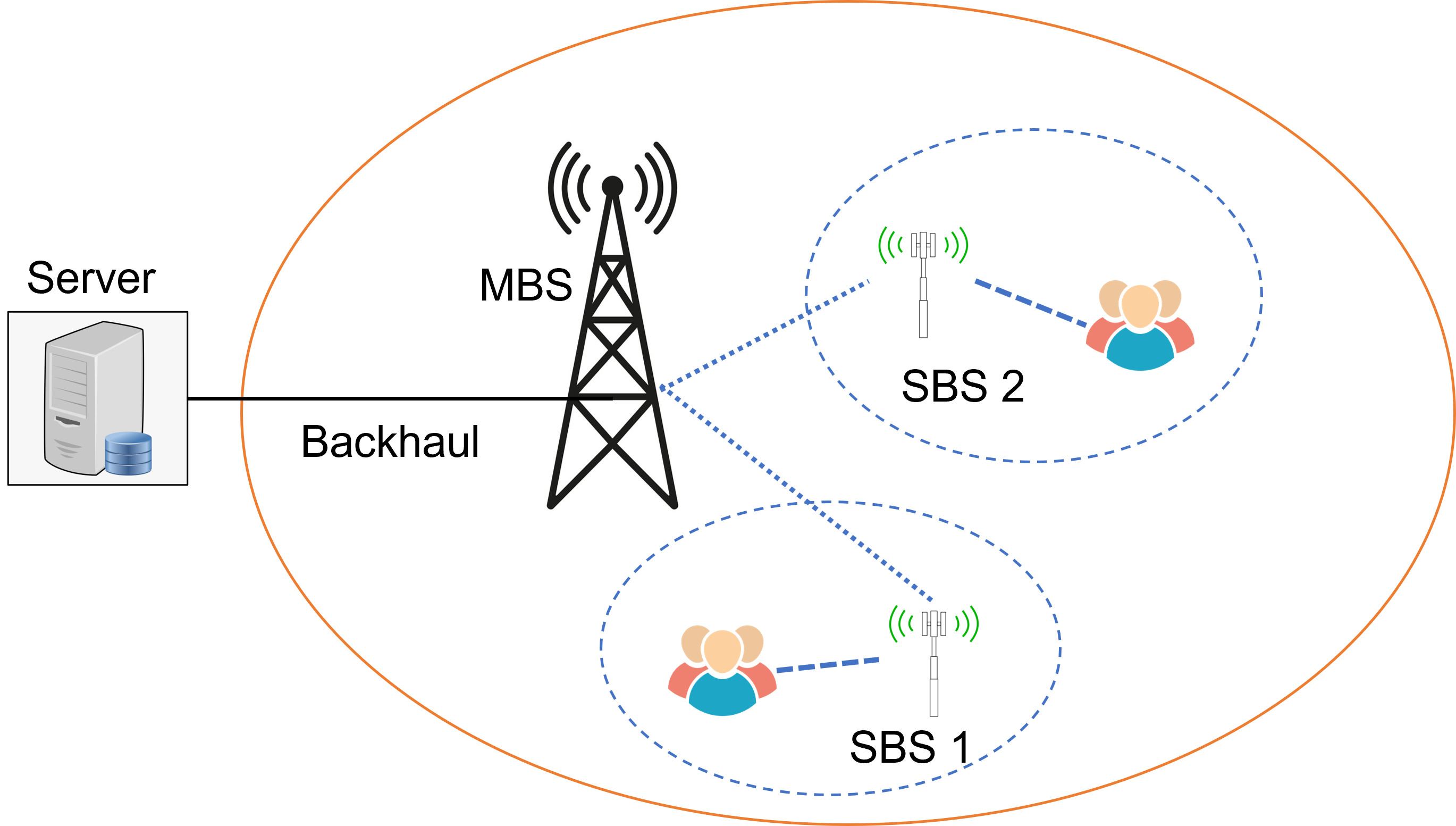
II System model

We consider a multi-cell network with one macro base station (MBS) and $N_{BS}$ small base stations (SBS), where each SBS serves multiple users. An example of this system is illustrated in Figure 1.

Figure 1: System model of the caching framework.

Each user requests contents from a fixed library. Let the content library be indexed by the set $\mathcal{F}=\left\{1,\ldots,F\right\}$, where each content is assumed to be of equal size .

In the time slot $t\in\left\{1,\ldots,T\right\}$, the $b^{th}$ SBS has a cache of size $L_{BS}$, and the $F\times 1$ vector $\mathbf{c}_{bt}$ describes the status of cache, that is, if the $f^{th}$ content is cached, $\mathbf{c}_{bt}(f)=1$ (else $0$ for not cached) with the cache size constraint $\mathbf{c}_{bt}^{T}\mathbf{1}_{F}=L_{BS}$. For fractional caching, where a portion of content is cached rather than the whole file, we have $\mathbf{c}_{bt}(f)\in\left[0,1\right]$ denoting the fraction of the $f^{th}$ content being cached, for each $f\in\mathcal{F}$. Before delivering the requested contents from users, a subset of popular contents are cached in the cache of the $b^{th}$ base station. Users are provided with the recommendations of the contents from library in a decreasing order of popularities at the local SBS. Based on the requested contents from the library, we define a direct hit to be the cache hit when the requested content is present in the cache, whereas indirect hits are the hits in cache for which users choose as an alternative to the requested content based on the recommendations when the requested content is unavailable in the cache. Each SBS collects the data about the direct and indirect hits for each time slot.

Let $\mathcal{D}_{t}=\big{\{}D_{fibj}\in\mathbb{R}_{+},\forall f,i\in\mathcal{F},b=1,\ldots,N_{BS},j=t-\tau+1,\ldots,t\big{\}}$ be a fourth-order tensor representing the aggregated data of number of direct and indirect content requests across all SBSs and for previous $\tau$ time slots ($t-\tau+1,\ldots,t$). The four dimensions of the tensor $\mathcal{D}_{t}$ respectively represent the requested content’s index, indices of requested contents based on recommendations, base station index, and time slot. In other words, in the $t^{th}$ time slot at $b^{th}$ BS, the number of recommended requests for the $i^{th}$ file, when the $f^{th}$ content is primarily requested, is denoted as $D_{fibt}$. Thus, the size of tensor is $I_{1}\times I_{2}\times I_{3}\times I_{4}$, where $I_{1}=I_{2}=F,\,I_{3}=N_{BS}$ and $I_{4}=\tau$. Note that only few entries of the tensor $\mathcal{D}_{t}$ can be observed, since the library is large and a few files are popular in a given time slot. Therefore, before processing this sparse tensor to derive the cache placement scheme, a tensor completion approach is essential. The following subsection describes the dynamics of the caching system.

II-A Edge caching procedures

The structure of the time slot is shown in Figure 2.

Figure 2: Time slot structure. CPL: content placement, CD: content delivery, IE: information exchange.

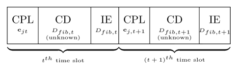
The first phase is the content placement (CPL) phase, where contents are placed in each BS’s cache based on the present information at base stations. The subsequent phase is the content delivery phase, where the content is delivered from the cache as per the requests from users. The next phase is dedicated for information exchange, where multiple base stations exchange the information about the number of hits and requests for better cache placements in the next time slot. For the CPL phase, the content placement strategy is chosen as a combination of two methods, that is, linear prediction of contents’ demands followed by most-popular caching (MPC) scheme. Since accurate prediction requires the data available for different contents, tensor completion problem is considered prior to performing prediction.

Moreover, in practice, the demands (number of requests for contents) are correlated across different contents and base stations, reducing the rank of the tensor $\mathcal{D}$. Thus, an independent prediction for individual base station and for each file can cause performance degradation. To deal with these correlation issues, authors in literature considers in-network caching [59], joint reinforcement learning [8], etc. However, in this work, we focus on improving the caching performance using tensor completion methods.

II-B Normalized cache hit rate and content placement

In literature [29, 16], to measure caching performance, several measures like cache hit (miss) rate, average success probability (ASP), etc have been considered. Improvements in these measures also relies on the prediction of demands. Cache hit rate at the $b^{th}$ base station in the $t^{th}$ time slot can be written as

$$\mathcal{H}_{bt}=\frac{\sum_{f,i\in\mathcal{F}}D_{fibt}\mathbf{c}_{bt}(f)}{\sum_{f,i\in\mathcal{F}}D_{fibt}},$$ (1)

which evaluates the cache placement policy.

Note that the number of requests at SBSs is random with unknown distribution, and not available in advance. That is, the decision for the $f^{th}$ file is set based on the previous number of requests. The objective of caching is to find the best content placement strategy to maximize the hit rate above. If in $(t+1)^{th}$ time slot the number of requests $D_{fib,t+1}$ is known in advance, we can choose $L_{BS}$ files with largest number of requests. On the other hand, when $D_{fib,t+1}$ is not known, it is natural to maximize the expected value given the previous information as

$$\arg\max_{\mathbf{c}_{b,t+1},\forall b}\mathbb{E}_{D}\left[\sum_{b}\mathcal{H}_{b,t+1}|\mathcal{D}_{t}\right]$$ (2a)

$$=\arg\max_{\mathbf{c}_{b,t+1},\forall b}\sum_{b}\sum_{f\in\mathcal{F}}\mathbf{c}_{bt}(f)\mathbb{E}_{D}\left[\frac{\sum_{i\in\mathcal{F}}D_{ifb,t+1}}{\sum_{f,i\in\mathcal{F}}D_{ifb,t+1}}|\mathcal{D}_{t}\right],$$ (2b)

in which $\mathbb{E}_{D}\left[\frac{\sum_{i\in\mathcal{F}}D_{ifb,t+1}}{\sum_{f,i\in\mathcal{F}}D_{ifb,t+1}}|\mathcal{D}_{t}\right]$ denotes the conditional mean estimate of the normalized number of requests. This estimate is the prediction of demands at $t+1$, given the past $\tau$ observations of demands until time slot $t$. Note that given the prediction estimates, the solution for caching strategy includes the $L_{BS}$ contents which have largest values in the estimate. To compute this estimate, the probability distribution of normalized requests must be known. However, the number of users’ requests are random and non-stationary with unknown distribution. Therefore, in the following, we obtain linear prediction estimation using least squares.

II-C Linear prediction

Let $\bar{D}_{fbt}=\frac{\sum_{i\in\mathcal{F}}D_{ifbt}}{\sum_{f,i\in\mathcal{F}}D_{ifbt}}$ denote the normalized number of requests, such that $\sum_{f\in\mathcal{F}}\bar{D}_{fbt}=1$. To obtain the linear predicton, the normalized demands are assumed to evolve as a linear combination of demands in the temporal dimension as

$$\bar{D}_{fb,t+1}\approx\sum_{m=1}^{M}c_{bm}\bar{D}_{fbm},\forall f\in\mathcal{F},$$ (3)

where $M$ is the order of prediction and $c_{bm}$ are the prediction coefficients. These coefficients are obtained by solving least squares fit problem, given the previous $\tau$ observations $\bar{D}_{fbj},j=t-\tau+1,\ldots,t$ for each $b$ as

$$\min_{c_{bi}\forall i} \sum_{f\in\mathcal{F}}\sum_{j=0}^{\tau-M-1}\left|\bar{D}_{fb,t-j}-\sum_{m=1}^{M}\bar{D}_{fb,t-j-m}c_{bm}\right|^{2}$$ (4a)

subject to $$\sum_{m=1}^{M}c_{bm}\bar{D}_{fbm}\geq 0,\forall f\in\mathcal{F}$$ (4b)

$$\sum_{f\in\mathcal{F}}\sum_{m=1}^{M}c_{bm}\bar{D}_{fbm}=1,$$ (4c)

where the constraints provides the non-negative values. Let the prediction estimate be denoted as $\hat{\bar{D}}_{fb,t+1}=\sum_{m=1}^{M}c_{bm}\bar{D}_{fbm}$. Mean based approach can be considered as a special case of linear prediction approach, i.e. $c_{bi}=\nicefrac{{1}}{{d}},\forall i=1,\ldots,d$. Since the data is sparse and correlated across files and base stations, it is difficult to directly obtain accurate predictions via these methods. Therefore, after filling the entries via tensor completion method, the above linear prediction can be used to find the future popularity estimates. For simplicity, in later sections, we recall this linear prediction method using the notation $\left\{\hat{\bar{D}}_{fb,t+1},\forall f,b\right\}\leftarrow LP\left\{\mathcal{D}_{t}\right\}$.

II-D Tensor preliminaries: Circular unfolding and folding

To efficiently represent the information in higher order tensors, authors in [52, 60] defined a balance unfolding scheme based on circular unfolding. For an $N$-order tensor $\mathcal{X}$, the tensor circular unfolding matrix, denoted by $\mathcal{X}_{(k,d)}$ of size $\bar{I}_{k}\times\bar{J}_{k}=I_{a}I_{a+1}\ldots I_{k}\times I_{k+1}\ldots I_{a-1}$, can be written as

$$\mathcal{X}_{\left(k,d\right)}\left(i_{a}i_{a+1}\ldots i_{k}\times i_{k+1}\ldots i_{a-1}\right)=\mathcal{X}\left(i_{1},i_{2},\ldots,i_{N}\right),$$ (5)

where $d$ is a positive integer and

$$a=\begin{cases}k-d+1,&d\leq k;\\ k-d+1+N,&d>k.\end{cases}$$ (6)

The above unfolding with the given mode $k$ and shift $d$ provides the balanced unfolding. Note that the balance of the above unfolding depends on the shift $d$. Similarly, the folding of a matrix $\mathbf{X}$ of size $I_{a}I_{a+1}\ldots I_{k}\times I_{k+1}\ldots I_{a-1}$ along the mode $k$ and shift $d$ provides the tensor $\left\llbracket\mathbf{X}\right\rrbracket_{\left(k,d\right)}$ of size $I_{1}\times\ldots\times I_{N}$.

II-E Latent nuclear norm with cyclic unfolding

The cyclic unfolding based latent nuclear norm is defined for an $N$-order tensor $\mathcal{X}$ as follows [36, 55]

$$\left\|\mathcal{X}\right\|_{TR}=\min_{\mathcal{X}_{1}+\ldots+\mathcal{X}_{N}=\mathcal{X}}\sum_{k=1}^{N}\left\|\mathcal{X}_{k,(k,d)}\right\|_{*},$$ (7)

where the minimum is over $N$ tensors $\left\{\mathcal{X}_{k}\right\}_{k=1}^{N}$, and $\mathcal{X}_{k,(k,d)}$ denotes the low-rank unfolding of $\mathcal{X}_{k}$ along the mode $k$ with a given value of $d$.

II-F Tensor completion problem

Let $\mathcal{T}\in\mathbb{R}^{I_{1}\times\cdots\times I_{N}}$ be an $N$-order sparse tensor with the observed entries. The location of entries in $\mathcal{T}$ is denoted by another indicator tensor $\mathcal{I}$, where $\mathcal{I}\left(i_{1},i_{2},\ldots,i_{N}\right)$ is 1 when $\mathcal{T}\left(i_{1},i_{2},\ldots,i_{N}\right)\neq 0$, and 0, otherwise. The notation $\left|\mathcal{I}\right|$ and $\mathcal{T}(\mathcal{I})$ define the number of non-zeros in the $\mathcal{I}$ and the entries of $\mathcal{T}$ for the corresponding non-zeros indices in $\mathcal{I}$, respectively.

The optimization problem for low-rank tensor completion using TR-latent nuclear norm is cast as

$$\min_{\mathcal{X}_{k},\forall k} \left\|\mathcal{X}\right\|_{TR}$$ (8a)

subject to $$\mathcal{X}=\sum_{k=1}^{N}\mathcal{X}_{k},\mathcal{X}(\mathcal{I})=\mathcal{T}(\mathcal{I}),$$ (8b)

where $\mathcal{X}_{k}$ are component tensors and unfolded cyclically. To solve the above optimization, recently in [55, 36], Frank Wolfe algorithm is used to obtain parameters independent iterative procedure for tensor completion. However, the computation complexity is large due to optimum mode selection $k$, which requires SVD of $\mathcal{X}_{k}$ along each of $N$ modes (since $k=1,\ldots,N$); and the iterative compression of basis matrices, where SVD, QR and a quadratic optimization is performed. In this work, we propose a procedure with much lower computational overhead and along with significantly better reconstruction error. The details are described in the following.

III Tensor completion algorithm

III-A Rank efficient modified FW algorithm

Under the Frank-Wolfe framework, the optimization problem in (8a) can be rewritten as

$$\min_{\mathcal{X}} F(\mathcal{X})$$ (9a)

subject to $$\left\|\mathcal{X}\right\|_{TR}\leq\beta,$$ (9b)

where $F(\mathcal{X})=\frac{1}{2}\left\|\mathcal{X}(\mathcal{I})-\mathcal{T}(\mathcal{I})\right\|_{F}^{2}$ and $\beta>0$. The constraint $\left\|\mathcal{X}\right\|_{TR}\leq\beta$ is also related to the rank constraint, that is, if the rank constraint is not specified, the rank of the solution can be high. However, for the proposed procedure, we will show that with the rank constraint specified, the above constraint can be relaxed; in other words, low rank solutions can be obtained with the specified $\beta$ limit.

The above optimization is solved via the gradient descent steps in the FW algorithm. It can be observed that the constraint $\mathcal{X}=\sum_{k=1}^{N}\mathcal{X}_{k}$ is also included in the TR-norm constraint. For the cyclic unfolding, we can write

$$\mathcal{X}=\sum_{k=1}^{N}\left\llbracket\mathcal{X}_{k,\left(k,d\right)}\right\rrbracket_{\left(k,d\right)},$$ (10)

where the matrices $\mathcal{X}_{k,\left(k,d\right)}$ are of low-rank, say $R_{k}$. Given the rank constraint of overall TC problem (say $R$), all $\mathcal{X}_{k}$ must satisfy $\sum_{k=1}^{N}R_{k}\leq R$. Note that for notational simplicity, we omit the iteration index. The update of the gradient descent can be given as

$$\mathcal{X}\leftarrow\mathcal{X}-\gamma\mathcal{S},$$ (11)

where $\gamma>0$ and the tensor $\mathcal{S}$ represent the gradient of $F(\mathcal{X})$, $\nabla F=\mathcal{X}(\mathcal{I})-\mathcal{T}(\mathcal{I}).$ The efficient representation of $F(\mathcal{X})$ with a decomposition and the TR-norm constraint can be obtained as follows.

III-A1 Constraint linear optimization

The problem of finding the tensor gradient of $F(\mathcal{X})$ to satisfy the constraint (9b) can be expressed as

$$\mathcal{S} =\arg\max_{\left\|\mathcal{S}\right\|_{TR}\leq\beta}\left\langle\mathcal{S},\nabla F\right\rangle,$$

where the objective is maximize the correlation between the above two tensors. Note that the objective function is linear. One possible solution is to choose $\mathcal{S}=\beta\frac{\nabla F}{\left\|\nabla F\right\|_{TR}}$. However, we also need low-rank decomposition of $\mathcal{S}$ for the tensor completion problem. Therefore, we first find the optimum mode for cyclic unfolding, and then, leverage SVD for decomposition components. To find the optimum mode, we compare the first dominant singular value of the unfolded tensor $\nabla F$ along different modes, that is,

$$k^{*}=\arg\max_{k}\sigma_{max}\left[\left(\nabla F\right)_{\left(k,d\right)}\right],$$

where the notation $\sigma_{max}(\mathbf{A})$ denotes the maximum eigenvalue of the matrix $\mathbf{A}$. Let the folded gradient has SVD as $\left(\nabla F\right)_{\left(k,d\right)}=\tilde{\mathbf{U}}_{k}\tilde{\Sigma}_{k}\tilde{\mathbf{V}}_{k}^{T}$, where the singular values are assumed in a descending order. For a low-rank tensor completion, rank is a constraint, say $r_{k}$. We will present how to obtain $r_{k}$ later. Therefore, we have the gradient solution as

$$\mathcal{S}=\beta\frac{\left\llbracket\tilde{\mathbf{U}}_{k^{*}}(1:r_{k^{*}})\tilde{\Sigma}_{k^{*}}(1:r_{k^{*}},1:r_{k^{*}})\tilde{\mathbf{V}}_{k^{*}}^{T}(1:r_{k^{*}})\right\rrbracket_{\left(k^{*},d\right)}}{\mathbf{1}_{r_{k^{*}}}^{T}\tilde{\Sigma}_{k^{*}}(1:r_{k^{*}},1:r_{k^{*}})\mathbf{1}_{r_{k^{*}}}},$$ (12)

where for a matrix $\mathbf{A}(1:m,1:n)$ denotes the submatrix with entries belonging to the first $m$ rows and first $n$ columns of $\mathbf{A}$; and $\mathbf{A}(1:n)$ is the submatrix with first $n$ columns of $\mathbf{A}$; $\mathbf{1}_{n}$ denotes $n\times 1$ vectors of ones.

Remark (rank-1 updates): For gradient representation $\mathcal{S}$, instead of choosing $r_{k}$ rank, rank-$1$ updates can be considered (for a suboptimal solution with larger overhead) as

$$\mathcal{S}=\beta\left\llbracket\tilde{\mathbf{U}}_{k^{*}}(1)\tilde{\mathbf{V}}_{k^{*}}^{T}(1)\right\rrbracket_{\left(k^{*},d\right)},$$ (13)

which is inefficient than as compared to (12) due to the fact that the structure of singular values $\tilde{\Sigma}_{k^{*}}$ is absent. Algorithm in [55, 36] gathers many such singular vector (and values), and find the structure of singular values via the compression step.

Remark (max-mode selection): In the above step, the mode $k^{*}$ is selected based on maximum singular value. For an $I_{1}\times\cdots\times I_{N}$ tensor, the singular value of an unfolding is maximum when its dimensions are minimum. If the $k^{th}$ unfolding has dimension $\bar{I}_{k}\times\bar{J}_{k}$, then the value $k^{*}$ can be selected as

$$k^{*}=\arg\min_{k}\min\left\{\bar{I}_{k},\bar{J}_{k}\right\},$$ (14)

which can significantly reduce the computational complexity of mode-selection, that is, the computations for $N$ singular values.

III-A2 Line search

The line search problem is to find the step size, which can be expressed as

$$\gamma =\arg\min_{\gamma\geq 0}\left\|\left\{\mathcal{X}\left(\mathcal{I}\right)-\gamma\mathcal{S}\right\}-\mathcal{T}\left(\mathcal{I}\right)\right\|_{F}^{2}$$ (15a)

$$=\arg\min_{\gamma\geq 0}\bar{a}\gamma^{2}-2\bar{b}\gamma$$ (15b)

$$=\max\left\{\frac{\bar{b}}{\bar{a}},0\right\},$$ (15c)

where $\bar{a}=\left\|\mathcal{S}\left(\mathcal{I}\right)\right\|_{F}^{2}$, $\bar{b}=\left\langle\mathcal{X}\left(\mathcal{I}\right)-\mathcal{T}\left(\mathcal{I}\right),\mathcal{S}\left(\mathcal{I}\right)\right\rangle$, and the solution is obtained by differentiation. The max-operator arises due to $\gamma\geq 0$ constraint. With $\gamma$ and $\mathcal{S}$ obtained, the tensor $\mathcal{X}$ can be updated using the equation (11).

III-A3 Decomposition update

Thanks to the decomposition, one does not need to store the whole tensor $\mathcal{S}$ or $\mathcal{X}$. We can store SVD components and step size as a representation of the update of the unfolded-component tensors. In other words, for the selected optimum mode-$k^{*}$, singular vectors along each mode are updated from, the update equation (11) can be simplified as

$$\mathcal{X}\leftarrow\mathcal{X}-\gamma\mathcal{S}$$ (16a)

$$=\sum_{k=1}^{N}\left\llbracket\mathcal{X}_{k,\left(k,d\right)}\right\rrbracket_{\left(k,d\right)}-\gamma\mathcal{S}$$ (16b)

$$=\sum_{k\neq k^{*}}\left\llbracket\mathcal{X}_{k,\left(k,d\right)}\right\rrbracket_{\left(k,d\right)}+\Bigg{\llbracket}\mathcal{X}_{k^{*},\left(k^{*},d\right)}-$$ (16c)

$$\gamma\beta\frac{\tilde{\mathbf{U}}_{k^{*}}(1:r_{k^{*}})\tilde{\Sigma}_{k^{*}}(1:r_{k^{*}},1:r_{k^{*}})\tilde{\mathbf{V}}_{k^{*}}^{T}(1:r_{k^{*}})}{\mathbf{1}_{r_{k^{*}}}^{T}\tilde{\Sigma}_{k^{*}}(1:r_{k^{*}},1:r_{k^{*}})\mathbf{1}_{r_{k^{*}}}}\Bigg{\rrbracket}_{\left(k^{*},d\right)}.$$

Since for each $k$, we have $\mathcal{X}_{k,\left(k,d\right)}=\mathbf{U}_{k}\boldsymbol{\Sigma}_{k}\mathbf{V}_{k}^{T}$, the above equation leads to the updation of singular vectors along only $k^{*}$-th mode as

$$\mathbf{U}_{k^{*}} \leftarrow\left[\mathbf{U}_{k^{*}},-\tilde{\mathbf{U}}_{k^{*}}(1:r_{k^{*}})\right],$$ (17a)

$$\mathbf{V}_{k^{*}} \leftarrow\left[\mathbf{V}_{k^{*}},\tilde{\mathbf{V}}_{k^{*}}(1:r_{k^{*}})\right],$$ (17b)

$$\boldsymbol{\Sigma}_{k^{*}} \leftarrow\left[\begin{array}[]{cc}\boldsymbol{\Sigma}_{k^{*}}&\mathbf{0}\\ \mathbf{0}&\frac{\gamma\beta\tilde{\Sigma}_{k^{*}}(1:r_{k^{*}},1:r_{k^{*}})}{\mathbf{1}_{r_{k^{*}}}^{T}\tilde{\Sigma}_{k^{*}}(1:r_{k^{*}},1:r_{k^{*}})\mathbf{1}_{r_{k^{*}}}}\end{array}\right],$$ (17e)

$$R_{k^{*}} \leftarrow R_{k^{*}}+r_{k^{*}},$$ (17f)

where the components $\mathbf{U}_{k},\boldsymbol{\Sigma}_{k},\mathbf{V}_{k},R_{k},k\neq k^{*}$ remains unchanged during this iteration. Regarding the update of $r_{k}$, there are two constraints, rank of the unfolded matrix $r_{k}\leq\min\left\{\bar{I}_{k},\bar{J}_{k}\right\}-R_{k}$, and the overall rank constraint $r_{k}\leq R-\sum_{k=1}^{N}R_{k}$. Thus, for the next iteration, the update for $r_{k}$ can be written as

$$r_{k}\leftarrow\min\left\{\bar{I}_{k}-R_{k},\bar{J}_{k}-R_{k},R-\sum_{i=1}^{N}R_{i}\right\},$$ (18)

which also defines the stopping criteria, that is, the iterative procedure stops if $r_{k}$ reaches $0$.

Remark (Compression step): It can be seen that due to rank constraint $r_{k}$, the above representation does not explode into many basis matrices. Thus, no-compression is required here, which significantly reduces the computational overhead, as compared to [55, 36]. Further, if the compression step is leveraged into the proposed algorithm, the reconstruction errors can be further reduced. However, for an online algorithm, this step is omitted.

III-A4 Algorithm

The Algorithm 1 presents the proposed TC procedure, which combines the steps obtained in the above subsections. In addition to the input observed tensor $\mathcal{T}$, the method requires to specify the required rank $R$ and the low-rank reconstruction error limit $\beta$. After the initialization of variables $\mathcal{X}=0$, $R_{k}=r_{k}=0,\mathbf{U}_{k}=\Sigma_{k}=\mathbf{V}_{k}=\emptyset,\forall k$, first the optimum mode $k^{*}$ is selected and the corresponding unfolded mode SVD of $\nabla F$ is computed. Based on the value of $r_{k}$, the gradient representation $\mathcal{S}$ and the step size $\gamma$ are calculated via rank-$r_{k}$ truncated SVD. Subsequently, the rest of variables are updated including $\mathcal{X}$, $\mathbf{U}_{k^{*}},\boldsymbol{\Sigma}_{k^{*}},\mathbf{V}_{k^{*}}$ and $R_{k^{*}}$. For usage, the algorithmic procedure is denoted as $\mathcal{X}\leftarrow TCA(\mathcal{T},R)$.

The value of $r_{k}$ denotes the number of available dimensions in the $k^{th}$ mode. The value $r_{k}=0$ means either, the overall rank constraint $R=\sum_{k}R_{k}$ is satisfied, or, mode-$k$ rank is reached, i.e., $R_{k}=\min\left\{\bar{I}_{k},\bar{J}_{k}\right\}$. The former constraint leads to the stopping criteria, while the latter adds the pruning step for the search space of optimum mode selection, that is, $\mathcal{N}\leftarrow\mathcal{N}\setminus\left\{k\right\}$.

Proposition 1.

Given the rank constraint $R$, the Algorithm 1 is independent of $\beta$.

Proof:

In the algorithm, the update equation (11) depends on the the product $\gamma\beta$. By the definition of $\gamma$, we write $\gamma=\frac{\left\langle\mathcal{X}\left(\mathcal{I}\right)-\mathcal{T}\left(\mathcal{I}\right),\mathcal{S}\left(\mathcal{I}\right)\right\rangle}{\left\|\mathcal{S}\left(\mathcal{I}\right)\right\|_{F}^{2}}.$ Substituting the value $\mathcal{S}$ from (12) provides $\beta\gamma=constant$, where the constant is specified via the singular values in the unfolding in $k^{*}$-mode of $\nabla F$. In other words, $\gamma$ adjusts itself according to $\beta$ in each iteration, leading to $\beta$-independent algorithm. This is also verified via simulations. ∎

1:$\mathcal{T}$, $\beta$, $R,d$.

2:$\mathbf{U}_{k},\boldsymbol{\Sigma}_{k},\mathbf{V}_{k},\forall k$:$\left\|\sum_{k=1}^{N}\left\llbracket\mathbf{U}_{k}\boldsymbol{\Sigma}_{k}\mathbf{V}_{k}^{T}\right\rrbracket_{\left(k,d\right)}\right\|_{TR}\leq\beta$.

3:Initialize $\mathcal{X}=0$, $R_{k}=r_{k}=0,\mathbf{U}_{k}=\Sigma_{k}=\mathbf{V}_{k}=\emptyset,\forall k$.

4:Initialize $\mathcal{N}=\left\{1,\dots,N\right\}.$

5:for $n=1,2,\ldots,n_{\max}$ do

6:     Set the tensor $\nabla F=\mathcal{X}(\mathcal{I})-\mathcal{T}(\mathcal{I})$.

7:     Obtain $k^{*}=\arg\max_{k\in\mathcal{N}}\sigma_{max}\left[\left(\nabla F\right)_{\left(k,d\right)}\right]$.

8:     Get the SVD $\left(\nabla F\right)_{\left(k^{*},d\right)}=\tilde{\mathbf{U}}_{k^{*}}\tilde{\Sigma}_{k^{*}}\tilde{\mathbf{V}}_{k^{*}}^{T}\in\mathbb{R}^{\bar{I}_{k^{*}}\times\bar{J}_{k^{*}}}$

9:     Update $r_{k}\leftarrow\min\left\{\bar{I}_{k}-R_{k},\bar{J}_{k}-R_{k},R-\sum_{k=1}^{N}R_{k}\right\}$.

10:     if $r_{k}\leq 0$ then

11:         Break the loop.

12:     end if

13:     Compute $\mathcal{S}$ from (12).

14:     Get step size $\gamma$ from (15c).

15:     Update $\mathcal{X}\leftarrow\mathcal{X}-\gamma\mathcal{S}$.

16:     Update $\mathbf{U}_{k^{*}},\boldsymbol{\Sigma}_{k^{*}},\mathbf{V}_{k^{*}}$.

17:     Update $R_{k^{*}}=R_{k^{*}}+r_{k^{*}}$.

18:     if $R_{k^{*}}=\min\left\{\bar{I}_{k^{*}},\bar{J}_{k^{*}}\right\}$ then

19:         $\mathcal{N}\leftarrow\mathcal{N}\setminus\left\{k^{*}\right\}$.

20:     end if

21:end for

22:Return $\mathbf{U}_{k},\boldsymbol{\Sigma}_{k},\mathbf{V}_{k},\forall k$.

Algorithm 1 Rank efficient modified FW algorithm, $TCA(\mathcal{T},R)$.

III-A5 Time and space complexity

Let $\mathcal{X}$ be an $N$-order tensor of dimension $I\times\ldots\times I$. In the algorithm 1, rank-$R$ SVD is computed for the cyclically unfolded matrix of size $I^{d}\times I^{N-d}$, which incurs the complexity $\mathcal{O}\left(I^{2d}I^{N-d}\right)=\mathcal{O}\left(I^{N+d}\right)$. Regarding space complexity for rank-$R$ decomposition, $I^{d}R+I^{N-d}R+R$ real valued space is required for $\mathbf{U}_{k},\mathbf{V}_{k},\Sigma_{k},\forall k$, and $\left|\mathcal{I}\right|$ space for the observable tensor.

III-B Online prediction and caching algorithm

Since the above tensor completion is fast, it can be used in an online manner for edge caching, as shown in the Algorithm 2. In this algorithm, the tensor completion and linear prediction methods are employed in the information exchange phase, whereas the cache placement phase is dedicated to placing the content according to the predicted number of normalized requests.

1:$\mathcal{D}_{t},\forall t$, $R$.

2:$\mathbf{c}_{bt},\forall b,t$

3:for $t=\tau,\tau+1,\ldots$ do

4:     IE phase: Observe the tensor $\mathcal{D}_{t}$.

5:     Apply $\mathcal{X}\leftarrow TCA(\mathcal{D}_{t},R)$.

6:     Employ $\left\{\hat{\bar{D}}_{fb,t+1},\forall f,b\right\}\leftarrow LP(\mathcal{X})$.

7:     CPL phase: Based on $\hat{\bar{D}}_{fb,t+1},\forall f$, obtain MPC placement $\mathbf{c}_{bt}$, for each $b$.

8:     CD phase: deliver contents from as per users’ requests.

9:end for

Algorithm 2 Online prediction and caching algorithm.

IV Simulation Results

Simulations are performed on the MovieLens dataset [61], where fourth order tensors ($N=4$) are constructed from the movie ratings with dimensions $F\times F\times N_{BS}\times\tau$, where $F=128$, $N_{BS}=3$, and $\tau=10$. Each time slot entry is set by aggregating the rating for 30 days based on the timestamps given. $M=6$-th order prediction is performed. For tensor completion, values $d=1$, $\beta=10^{5}$, $R=nN$, $n=2,4,6,8,10,12$ are chosen. For edge caching, $L_{BS}=32$ is chosen. The algorithm is compared for normalized reconstruction errors, defined as

$$RSE=\frac{\left\|\mathcal{X}(\mathcal{I})-\mathcal{T}(\mathcal{I})\right\|_{F}}{\left\|\mathcal{T}(\mathcal{I})\right\|_{F}},$$ (19)

which equals to $1$ at the start of first iteration, since $\mathcal{X}=0$. . Two prediction methods are chosen, that is, linear predictions with optimum coefficients (LP) and with equal coefficients (MP). The performance of edge caching is measured in terms of cache hit rate. Algorithms are run on a windows PC with Intel Xeon CPU E3-1230 v5 (3.40GHz, 32GB RAM).

IV-A Convergence

Figure 3: RSE versus the execution time (in MATLAB) for the proposed algorithm and the algorithm in [55], for $\beta=10^{5}$ and $R=nN$, $\forall n=2,4,6,8,10,12$.

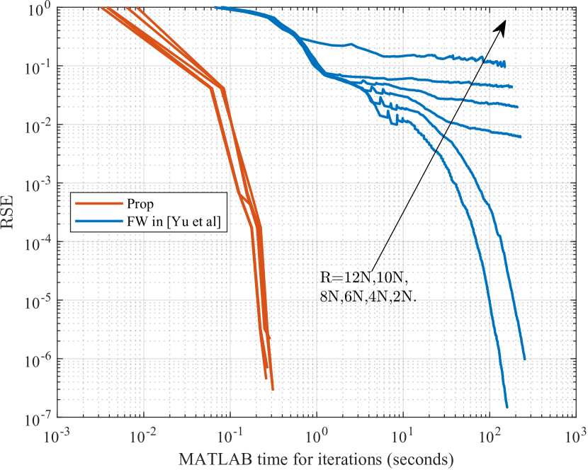
Figure 3 plots the convergence in terms of RSE for the proposed algorithm, and the FW algorithm in [55] for $\beta=10^{5}$ and $R=nN$, $\forall n=2,4,6,8,10,12$. It can be observed that the proposed algorithm outperforms significantly as compared to the one in [55]. It achieves less RSE in less iterations (e.g. at $R=2N=32$, $RSE\approx 10^{-1}$ for Yu et al, and $RSE<10^{-6}$ for the proposed one), and each iteration executes in less time as well (total time is 0.2 seconds versus 200 seconds approximately).

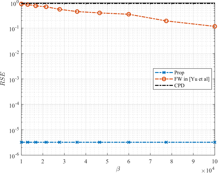
IV-B Effect of latent factors $R$ and $\beta$

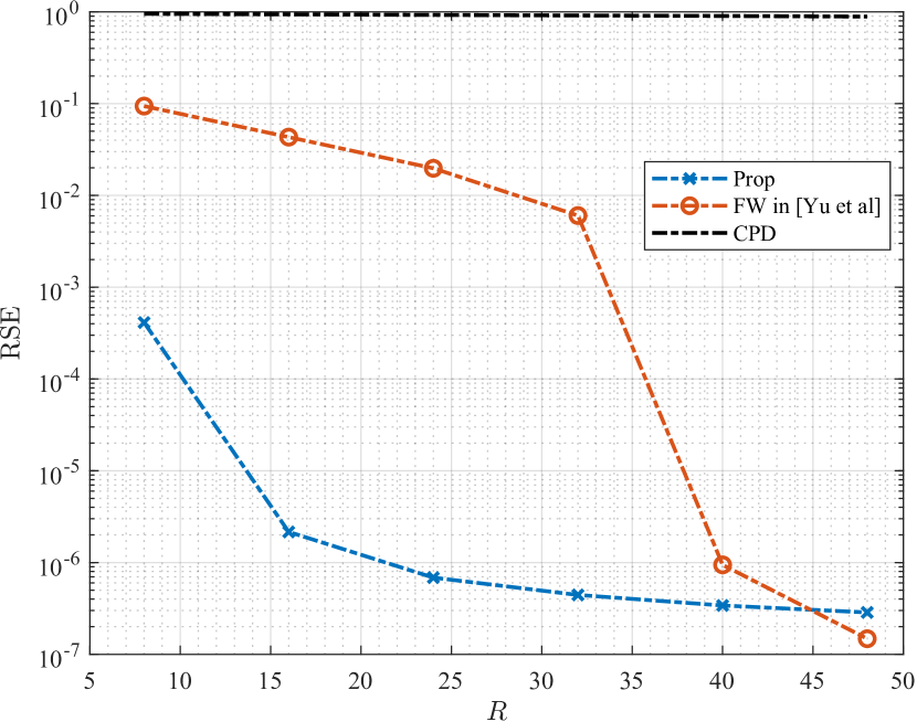
To observe the effect of the factor $\beta$, Figure 4 plots the RSE with respect to $\beta$ at $R=6N$ for all the three methods, while Figure 5 shows with respect to the rank $R$ with the fixed $\beta=10^{5}$. It can be seen that for all values of $\beta$, the proposed algorithm provides much less RSE than for CPD and the method in [55]. Moreover, the proposed algorithm is invariant to changes in $\beta$, as shown in Proposition 1. Regarding the plots versus rank-$R$, the proposed method performs significantly better at lower ranks. As the rank is increased, the performance difference between the proposed and the FW algorithm decreases. For sufficiently high rank $R>45$, FW provides minutely better performance, where the difference in RSE is the order of $10^{-6}$.

Figure 4: Relative and reconstruction errors with respect to $\beta$ at $R=6N$.

Figure 5: Relative and reconstruction errors versus different ranks with fixed $\beta$.

IV-C Cache hit rate

Figure 6: Average cache hit rate for two linear prediction methods with three different completion methods for MovieLens dataset with $R=2N,4N,6N$ ranks and $\beta=10^{5}$.

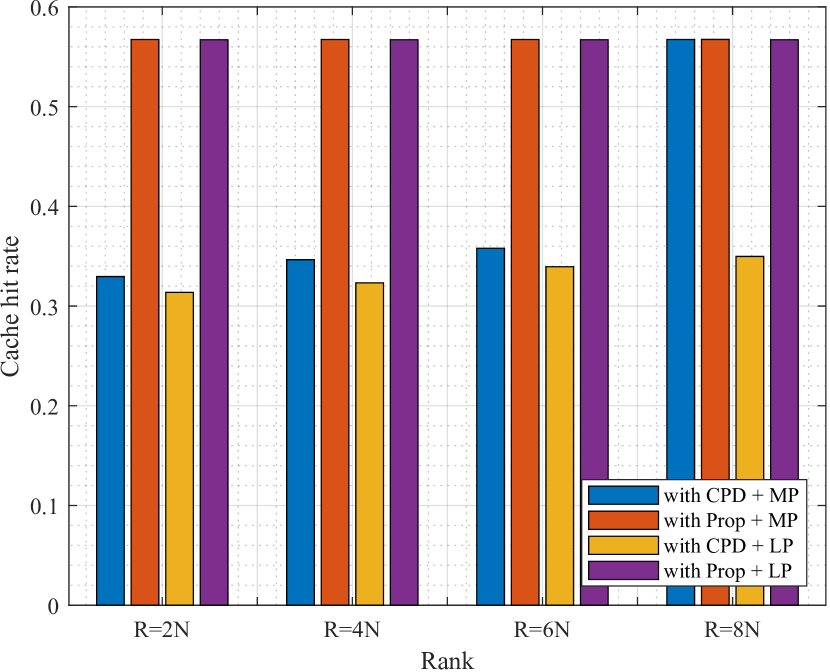
To evaluate the performance of the proposed method for edge caching scenario, Figure 6 shows the normalized cache hit rates averaged across time slots for three different methods with the cache size of $32$. The results are averaged over 220 time slots, wherein each time slot a tensor completion problem is solved and future popularity is predicted using linear prediction (LP) and mean-prediction (MP) methods. It can be observed that as compared to CPD, the CHR improvement is around 75.8%. Mean prediction and linear prediction perform approximately similar for CHR. As the rank of completion is increased, improvements in the CHR remains similar, which is due to rank-efficient tensor completion. In other words, the proposed low-rank completion is efficient at low ranks; and so, the completion at higher ranks yields similar CHR performance, which can also be concluded from Figure 5.

V Conclusion

In this paper, we have proposed an improved time complexity based modified FW algorithm based on gradient descent, which has been shown to significantly outperform in term of computational complexity and performance. This algorithm needs only a few iterations, which is of the order of the specified rank $R$. Further, for the wireless edge caching, we have formulated content recommendation and prediction problem into a tensor completion framework. Using the completed tensor, we have employed linear prediction methods to obtain future popularities. For this application, it is shown via simulations that after completion, the algorithm provides significantly better cache hit rate (75%) as compared to the CP decomposition.

For the edge caching, the library size is typically large of the order of $10^{4}$. Performing tensor completion on such a large tensor is both time and space intensive. Therefore, in future, we shall explore to find the independent blocks in the observed tensor. It will significantly reduce the time and space requirements and better tensor decomposition can be found for the remaining block tensors as compared to the full tensor.

References

- [1] H. S. Goian, O. Y. Al-Jarrah, S. Muhaidat, Y. Al-Hammadi, P. Yoo, and M. Dianati, “Popularity-based video caching techniques for cache-enabled networks: A survey,” IEEE Access, vol. 7, pp. 27 699–27 719, 2019.
- [2] L. Li, G. Zhao, and R. S. Blum, “A survey of caching techniques in cellular networks: Research issues and challenges in content placement and delivery strategies,” IEEE Communications Surveys & Tutorials, vol. 20, no. 3, pp. 1710–1732, 2018.
- [3] K. Shanmugam, N. Golrezaei, A. G. Dimakis, A. F. Molisch, and G. Caire, “Femtocaching: Wireless content delivery through distributed caching helpers,” IEEE Transactions on Information Theory, vol. 59, no. 12, pp. 8402–8413, 2013.
- [4] K. Poularakis and L. Tassiulas, “On the complexity of optimal content placement in hierarchical caching networks,” IEEE Transactions on Communications, vol. 64, no. 5, pp. 2092–2103, 2016.
- [5] B. Blaszczyszyn and A. Giovanidis, “Optimal geographic caching in cellular networks,” in IEEE International Conference on Communications (ICC), 2015, pp. 3358–3363.
- [6] B. Serbetci and J. Goseling, “Optimal geographical caching in heterogeneous cellular networks with nonhomogeneous helpers,” arXiv preprint arXiv:1710.09626, 2017.
- [7] A. Papazafeiropoulos and T. Ratnarajah, “Modeling and performance of uplink cache-enabled massive mimo heterogeneous networks,” IEEE Transactions on Wireless Communications, vol. 17, no. 12, pp. 8136–8149, 2018.
- [8] A. Sadeghi, F. Sheikholeslami, and G. B. Giannakis, “Optimal and scalable caching for 5G using reinforcement learning of space-time popularities,” IEEE Journal of Selected Topics in Signal Processing, vol. 12, no. 1, pp. 180–190, 2018.
- [9] N. Garg, M. Sellathurai, V. Bhatia, and T. Ratnarajah, “Function approximation based reinforcement learning for edge caching in massive mimo networks,” IEEE Transactions on Communications, 2020.
- [10] J. Yin, L. Li, H. Zhang, X. Li, A. Gao, and Z. Han, “A prediction-based coordination caching scheme for content centric networking,” in WOCC, 2018, pp. 1–5.
- [11] W.-X. Liu, J. Zhang, Z.-W. Liang, L.-X. Peng, and J. Cai, “Content popularity prediction and caching for ICN: A deep learning approach with SDN,” IEEE Access, vol. 6, pp. 5075–5089, 2018.
- [12] H. Nakayama, S. Ata, and I. Oka, “Caching algorithm for content-oriented networks using prediction of popularity of contents,” in IFIP/IEEE International Symposium on Integrated Network Management (IM), 2015, pp. 1171–1176.
- [13] Y. Zhang, X. Tan, and W. Li, “Ppc: Popularity prediction caching in icn,” IEEE Communications Letters, vol. 22, no. 1, pp. 5–8, Jan 2018.
- [14] R. Haw, S. M. A. Kazmi, K. Thar, M. G. R. Alam, and C. S. Hong, “Cache aware user association for wireless heterogeneous networks,” IEEE Access, vol. 7, pp. 3472–3485, 2019.
- [15] J. Wu, Y. Zhou, D. M. Chiu, and Z. Zhu, “Modeling dynamics of online video popularity,” IEEE Transactions on Multimedia, vol. 18, no. 9, pp. 1882–1895, Sep. 2016.
- [16] Y. Jiang, M. Ma, M. Bennis, F. Zheng, and X. You, “User preference learning-based edge caching for fog radio access network,” IEEE Transactions on Communications, vol. 67, no. 2, pp. 1268–1283, Feb 2019.
- [17] Y. Wang, M. Ding, Z. Chen, and L. Luo, “Caching placement with recommendation systems for cache-enabled mobile social networks,” IEEE Communications Letters, vol. 21, no. 10, pp. 2266–2269, 2017.
- [18] P. Sermpezis, T. Giannakas, T. Spyropoulos, and L. Vigneri, “Soft cache hits: Improving performance through recommendation and delivery of related content,” IEEE Journal on Selected Areas in Communications, vol. 36, no. 6, pp. 1300–1313, 2018.
- [19] L. E. Chatzieleftheriou, M. Karaliopoulos, and I. Koutsopoulos, “Jointly optimizing content caching and recommendations in small cell networks,” IEEE Transactions on Mobile Computing, vol. 18, no. 1, pp. 125–138, 2019.
- [20] P. Cheng, C. Ma, M. Ding, Y. Hu, Z. Lin, Y. Li, and B. Vucetic, “Localized small cell caching: A machine learning approach based on rating data,” IEEE Transactions on Communications, vol. 67, no. 2, pp. 1663–1676, 2019.
- [21] K. Guo and C. Yang, “Temporal-spatial recommendation for caching at base stations via deep reinforcement learning,” IEEE Access, vol. 7, pp. 58 519–58 532, 2019.
- [22] W. He, Y. Su, X. Xu, Z. Luo, L. Huang, and X. Du, “Cooperative content caching for mobile edge computing with network coding,” IEEE Access, vol. 7, pp. 67 695–67 707, 2019.
- [23] S. Mehrizi, T. X. Vu, S. Chatzinotas, and B. Ottersten, “Trend-aware proactive caching via tensor train decomposition: A bayesian viewpoint,” IEEE Open Journal of the Communications Society, vol. 2, pp. 975–989, 2021.
- [24] N. Garg and T. Ratnarajah, “Tensor completion based prediction in wireless edge caching,” in 2020 54th Asilomar Conference on Signals, Systems, and Computers, 2020, pp. 1579–1582.
- [25] L. Cai, X. Wang, J. Wang, M. Huang, and T. Yang, “Multidimensional data learning-based caching strategy in information-centric networks,” in 2017 IEEE International Conference on Communications (ICC), May 2017, pp. 1–6.
- [26] J. Yang, Z. Yao, B. Yang, X. Tan, Z. Wang, and Q. Zheng, “Software-defined multimedia streaming system aided by variable-length interval in-network caching,” IEEE Transactions on Multimedia, vol. 21, no. 2, pp. 494–509, 2019.
- [27] Y. Zhu, G. Zheng, L. Wang, K. Wong, and L. Zhao, “Performance analysis and optimization of cache-enabled small cell networks,” in GLOBECOM 2017 - 2017 IEEE Global Communications Conference, Dec 2017, pp. 1–6.
- [28] N. Garg, M. Sellathurai, and T. Ratnarajah, “Content placement learning for success probability maximization in wireless edge caching networks,” in IEEE ICASSP, May 2019, pp. 3092–3096.
- [29] N. Garg, M. Sellathurai, V. Bhatia, B. N. Bharath, and T. Ratnarajah, “Online content popularity prediction and learning in wireless edge caching,” IEEE Transactions on Communications, vol. 68, no. 2, pp. 1087–1100, 2020.
- [30] N. Garg, V. Bhatia, B. Bettagere, M. Sellathurai, and T. Ratnarajah, “Online learning models for content popularity prediction in wireless edge caching,” arXiv preprints, 2019.
- [31] Y. Liu, Z. Long, H. Huang, and C. Zhu, “Low cp rank and tucker rank tensor completion for estimating missing components in image data,” IEEE Transactions on Circuits and Systems for Video Technology, vol. 30, no. 4, pp. 944–954, 2020.
- [32] T. Yokota and H. Hontani, “Simultaneous tensor completion and denoising by noise inequality constrained convex optimization,” IEEE Access, vol. 7, pp. 15 669–15 682, 2019.
- [33] B. Romera-Paredes and M. Pontil, “A new convex relaxation for tensor completion,” in Advances in Neural Information Processing Systems, 2013, pp. 2967–2975.
- [34] Y. Liu, F. Shang, L. Jiao, J. Cheng, and H. Cheng, “Trace norm regularized candecomp/parafac decomposition with missing data,” IEEE Transactions on Cybernetics, vol. 45, no. 11, pp. 2437–2448, 2015.
- [35] R. Jenatton, N. L. Roux, A. Bordes, and G. R. Obozinski, “A latent factor model for highly multi-relational data,” in Advances in neural information processing systems, 2012, pp. 3167–3175.
- [36] X. Guo, Q. Yao, and J. T.-Y. Kwok, “Efficient sparse low-rank tensor completion using the frank-wolfe algorithm,” in Thirty-First AAAI Conference on Artificial Intelligence, 2017.
- [37] E. Frolov and I. Oseledets, “Tensor methods and recommender systems,” WIREs Data Mining and Knowledge Discovery, vol. 7, no. 3, p. e1201, 2017. [Online]. Available: https://onlinelibrary.wiley.com/doi/abs/10.1002/widm.1201
- [38] V. N. Ioannidis, A. S. Zamzam, G. B. Giannakis, and N. D. Sidiropoulos, “Coupled graph and tensor factorization for recommender systems and community detection,” IEEE Transactions on Knowledge and Data Engineering, 2019.
- [39] R. Bro, “Parafac. tutorial and applications,” Chemometrics and Intelligent Laboratory Systems, vol. 38, no. 2, pp. 149–171, 1997. [Online]. Available: http://www.sciencedirect.com/science/article/pii/S0169743997000324
- [40] L. R. Tucker, “Some mathematical notes on three-mode factor analysis,” Psychometrika, vol. 31, no. 3, pp. 279–311, 1966.
- [41] E. Acar, D. M. Dunlavy, T. G. Kolda, and M. Morup, “Scalable tensor factorizations for incomplete data,” Chemometrics and Intelligent Laboratory Systems, vol. 106, no. 1, pp. 41–56, Mar 2011. [Online]. Available: http://dx.doi.org/10.1016/j.chemolab.2010.08.004
- [42] Q. Zhao, L. Zhang, and A. Cichocki, “Bayesian cp factorization of incomplete tensors with automatic rank determination,” IEEE Transactions on Pattern Analysis and Machine Intelligence, vol. 37, no. 9, pp. 1751–1763, 2015.
- [43] Y. Chen, C. Hsu, and H. M. Liao, “Simultaneous tensor decomposition and completion using factor priors,” IEEE Transactions on Pattern Analysis and Machine Intelligence, vol. 36, no. 3, pp. 577–591, 2014.
- [44] Q. Zhao, G. Zhou, S. Xie, L. Zhang, and A. Cichocki, “Tensor ring decomposition,” arXiv preprint arXiv:1606.05535, 2016.
- [45] Q. Zhao, M. Sugiyama, L. Yuan, and A. Cichocki, “Learning efficient tensor representations with ring-structured networks,” in ICASSP 2019-2019 IEEE International Conference on Acoustics, Speech and Signal Processing (ICASSP). IEEE, 2019, pp. 8608–8612.
- [46] Y. Chen, T. Huang, W. He, N. Yokoya, and X. Zhao, “Hyperspectral image compressive sensing reconstruction using subspace-based nonlocal tensor ring decomposition,” IEEE Transactions on Image Processing, vol. 29, pp. 6813–6828, 2020.
- [47] Y. Chen, W. He, N. Yokoya, T. Huang, and X. Zhao, “Nonlocal tensor-ring decomposition for hyperspectral image denoising,” IEEE Transactions on Geoscience and Remote Sensing, vol. 58, no. 2, pp. 1348–1362, 2020.
- [48] L. Yuan, J. Cao, X. Zhao, Q. Wu, and Q. Zhao, “Higher-dimension tensor completion via low-rank tensor ring decomposition,” in 2018 Asia-Pacific Signal and Information Processing Association Annual Summit and Conference (APSIPA ASC), 2018, pp. 1071–1076.
- [49] W. Wang, V. Aggarwal, and S. Aeron, “Efficient low rank tensor ring completion,” in 2017 IEEE International Conference on Computer Vision (ICCV), 2017, pp. 5698–5706.
- [50] J. Liu, P. Musialski, P. Wonka, and J. Ye, “Tensor completion for estimating missing values in visual data,” IEEE Transactions on Pattern Analysis and Machine Intelligence, vol. 35, no. 1, pp. 208–220, 2013.
- [51] J. A. Bengua, H. N. Phien, H. D. Tuan, and M. N. Do, “Efficient tensor completion for color image and video recovery: Low-rank tensor train,” IEEE Transactions on Image Processing, vol. 26, no. 5, pp. 2466–2479, 2017.
- [52] J. Yu, C. Li, Q. Zhao, and G. Zhou, “Tensor-ring nuclear norm minimization and application for visual : Data completion,” ICASSP 2019 - 2019 IEEE International Conference on Acoustics, Speech and Signal Processing (ICASSP), pp. 3142–3146, 2019.
- [53] R. Tomioka and T. Suzuki, “Convex tensor decomposition via structured schatten norm regularization,” in Advances in Neural Information Processing Systems 26, C. J. C. Burges, L. Bottou, M. Welling, Z. Ghahramani, and K. Q. Weinberger, Eds. Curran Associates, Inc., 2013, pp. 1331–1339. [Online]. Available: http://papers.nips.cc/paper/4985-convex-tensor-decomposition-via-structured-schatten-norm-regularization.pdf
- [54] A. Wang, X. Song, X. Wu, Z. Lai, and Z. Jin, “Latent schatten tt norm for tensor completion,” in ICASSP 2019 - 2019 IEEE International Conference on Acoustics, Speech and Signal Processing (ICASSP), 2019, pp. 2922–2926.
- [55] J. Yu, W. Sun, Y. Qiu, and Y. Huang, “An efficient tensor completion method via new latent nuclear norm,” IEEE Access, vol. 8, pp. 126 284–126 296, 2020.
- [56] M. Jaggi, “Revisiting Frank-Wolfe: Projection-free sparse convex optimization,” in Proceedings of the 30th International Conference on Machine Learning, ser. Proceedings of Machine Learning Research, S. Dasgupta and D. McAllester, Eds., vol. 28, no. 1. Atlanta, Georgia, USA: PMLR, 17–19 Jun 2013, pp. 427–435. [Online]. Available: http://proceedings.mlr.press/v28/jaggi13.html
- [57] N. Vervliet, O. Debals, L. Sorber, M. Van Barel, and L. De Lathauwer. (2016, Mar.) Tensorlab 3.0. Available online. [Online]. Available: https://www.tensorlab.net
- [58] L. Yuan, C. Li, D. Mandic, J. Cao, and Q. Zhao, “Tensor ring decomposition with rank minimization on latent space: An efficient approach for tensor completion,” 2018.
- [59] N. Garg, M. Sellathurai, and T. Ratnarajah, “In-network caching for hybrid satellite-terrestrial networks using deep reinforcement learning,” in ICASSP 2020 - 2020 IEEE International Conference on Acoustics, Speech and Signal Processing (ICASSP), 2020, pp. 8797–8801.
- [60] J. Yu, G. Zhou, Q. Zhao, and K. Xie, “An effective tensor completion method based on multi-linear tensor ring decomposition,” in 2018 Asia-Pacific Signal and Information Processing Association Annual Summit and Conference (APSIPA ASC), 2018, pp. 1344–1349.
- [61] F. M. Harper and J. A. Konstan, “The movielens datasets: History and context,” ACM Trans. Interact. Intell. Syst., vol. 5, no. 4, pp. 19:1–19:19, Dec. 2015. [Online]. Available: http://doi.acm.org/10.1145/2827872