Theory of heterogeneous circuits with stochastic memristive devices
Abstract
We introduce an approach based on the Chapman-Kolmogorov equation to model heterogeneous stochastic circuits, namely, the circuits combining binary or multi-state stochastic memristive devices and continuum reactive components (capacitors and/or inductors). Such circuits are described in terms of occupation probabilities of memristive states that are functions of reactive variables. As an illustrative example, the series circuit of a binary memristor and capacitor is considered in detail. Some analytical solutions are found. Our work offers a novel analytical/numerical tool for modeling complex stochastic networks, which may find a broad range of applications.
I Introduction
The well-known cycle-to-cycle variability of memristive devices is one of the major obstacles for their use in non-volatile memories and other potential applications. While, traditionally, the memristive devices (memristors) and their circuits have been mostly described in terms of deterministic models Chua and Kang (1976); Kvatinsky et al. (2015); Pershin et al. (2009); Strachan et al. (2013), there is a growing evidence that at least in a certain large group of memristive devices (such as the electrochemical metallization (ECM) cells Valov et al. (2011)) the resistance switching occurs stochastically, namely, at a random time interval from the pulse edge Jo et al. (2009); Gaba et al. (2013, 2014). Theoretically, the randomness in the resistance switching was implemented in several models Menzel et al. (2014); Naous and Salama (2016); Dowling et al. (2021, 2020); Ntinas et al. (2020).
Mathematically, stochastic processes can be described by introducing a noise term Van Kampen (2007) into the equations of memristor dynamics. Usually these noise terms correspond to a white or, in a more complicated case, colored noise. In the case of linear equations (with respect to the internal state variables), the noisy dynamics can be effectively analysed or even solved analytically. For non-linear stochastic differential equations, mainly numerical solutions can be found. This complicates tremendously the analysis of general properties of processes that such equations describe. In the cases when the stochastic processes are markovian, the evolution of probability distributions can be described by a master equation, which was first applied to stochastic memristive networks by the present authors together with V. Dowling Dowling et al. (2021). However, the application range of such approach Dowling et al. (2021) is limited to circuits composed of binary or multi-state stochastic memristors, current and/or voltage sources, and non-linear components such as diodes.
The purpose of the present paper is to generalize the method of master equation Dowling et al. (2021) to more complex circuits that include also capacitors and/or indictors. Our main goal is to understand the behavior of complex stochastic circuits on average, as each particular realization of the circuit dynamics is not representative of the circuit behavior overall (as it depends on the particular realization of switching probabilities). The difficulty stems from the fact that in any particular realization of circuit dynamics, the switching of memristive components depends on the values of reactive variables, and vice-versa. Therefore, the statistical description is also necessary for the description of reactive variables. For this purpose, we utilize a set of probability distribution functions.
This paper is organized in the following sections. In Sec. II, the model of binary and multi-state stochastic memristors is presented. Section III is the main part of this work, where the evolution equations for a binary memristor-capacitor circuit are derived from the Chapman-Kolmogorov equation (Subsec. III.1), and their analytical solutions are found (Subsec. III.2). The application of Sec. III approach to more complex circuits is discussed in Sec. IV that concludes.
II Stochastic memristor model
In the present paper we consider discrete stochastic memristors, whose resistance is characterized by values , . The transitions between two states, and , are described in terms of the voltage-dependent transition rates, , where is the voltage across the memristor. Only transitions between the adjacent states are allowed (e. g., , , …, at , etc.). The transition from one boundary state to another occurs sequentially through all intermediate states.
The binary stochastic memristors Dowling et al. (2021) are the simplest case of discrete stochastic memristors. Experiments have shown Jo et al. (2009); Gaba et al. (2013, 2014) that in some electrochemical metallization cells the switching can be described by a probabilistic model with voltage-dependent switching rates
| (3) | |||
| (6) |
Here, and are constants. The interpretation of the above equations is following: The probability to switch from (state 0) to (state 1) within the infinitesimal time interval is . The probability to switch in the opposite direction is defined similarly. Equations similar to Eqs. (3)-(6) can be used for multi-state () stochastic memristors Dowling et al. (2020); Ntinas et al. (2020).
III Binary Memristor-Capacitor Circuit
In this Section we consider the circuit shown in Fig. 1(a), where M is a stochastic binary memristor (described by Eqs. (3) and (6)), and C is a linear capacitor. It is assumed that the circuit is driven by a time-dependent voltage .
III.1 Dynamical equations
The circuit description is based on the probability distribution functions, , . The meaning of these functions is that is the probability to find the memristor in state , and capacitor charge in the interval from to at time . For the full probabilistic description of memristive switching it is necessary to introduce the transition probabilities from the memristor state and capacitor charge at time to the memristor state and capacitor charge at time .
The Chapman-Kolmogorov equation Van Kampen (2007) describing the Markov process of stochastic switching can be written as
| (7) |
In order to satisfy the normalization condition at any time
| (8) |
the transition probabilities must satisfy for any , , , and the corresponding conditions
| (9) |
It is easy to find the transition probabilities for infinitesimally small . There are four transition probabilities as the memristive system is binary. For example, the transitional probability for switching from to is equal to
| (10) |
where is the voltage drop across the memristor, and the Dirac delta function represents the change in the capacitor charge that is defined by Kirchhoff’s law
| (11) |
(a)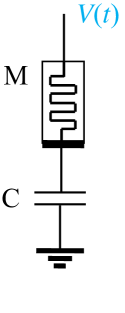 (b)
(b)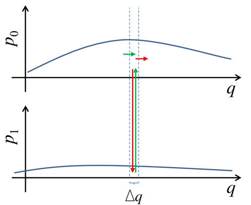
Then, for the transitional probability from to (no switching) we can write (similarly to Eq. (10))
| (12) |
The transitional probabilities and are obtained by replacing and in Eqs. (10) and (12). Note that such expressions for the transitional probabilities satisfy normalization conditions (9). Also we should note that Eqs. (10) and (12) are valid only up to the first order of magnitude of time , i.e. we should omit -terms or higher while using these equations.
By substituting Eqs. (10) and (12) into the Chapman-Kolmogorov equation (7) with , and expanding it with respect to up to the first order in magnitude, we get the following partial differential equation for the probability distribution function
| (13) |
where is the voltage across the memristor.
The other equation is obtained by replacing and in Eq. (13):
| (14) |
The system of Eqs. (13) and (14) must be supplemented with the initial distributions: and .
We note that Eqs. (13) and (14) can be considered as generalized continuity equations. Schematically, the interpretation of various terms in Eq. (13) is presented in Fig. 1(b). The second term in the left-hand side of Eq. (13) describes the flow of probability density through the boundaries of a small charge interval (the horizontal arrows in Fig. 1(b)). The right-hand side of Eq. (13) represents the flow of probability density between and (the vertical arrows in Fig. 1(b)).
III.2 Analytical solutions
While the fundamental solution of Eqs. (13) and (14) delivers the complete description of circuit behavior, it cannot be found analytically in a closed form for an arbitrary . Thus we confine ourselves to some important particular cases, when such solution can be found. They are i) the limit of small voltages when no transition occurs, and ii) unidirectional switching case, when transitions go only from one state to another.
III.2.1 No switching case
For those moments of time , capacitor charge , and applied voltage when no switching practically occurs, Eqs. (13)-(14) can be simplified to the following independent equations:
| (15) | |||
| (16) |
The general solution of Eqs. (15)-(16) can be found by the method of characteristics Strauss (2007) and presented as
| (17) |
| (18) |
where and are two arbitrary functions (initial conditions). We reiterate that Eqs. (17) and (18) with and provide the full solution in the case when the transitions between the states can be neglected.
To illustrate the above solution, we consider the step-like initial probability distribution
| (19) | |||||
| (20) |
Then in accordance with Eq. (17) we get the following expression for the charge probability distribution at any moment of time:
| (21) | |||
| (22) |
where
| (23) |
with . Eq. (23) is similar to the time-dependence of capacitor charge in the classical RC-circuit subjected to the voltage .
From Eq. (22) we see that the dissipative nature of memristor-capacitor circuit leads to the exponential narrowing of the probability distributions with time. At long times, , the distribution approaches Dirac delta function
| (24) |
It is clear Eq. (24) is valid for any initial distribution in the absence of resistance switching events.
III.2.2 Unidirectional switching
Next we consider the region in phase plane, where the transitions from to are forbidden, but the opposite transitions may occur. In this situation Eqs. (13) and (14) can be rewritten as
| (28) | |||||
| (29) |
Eqs. (28) and (29) are valid when . The general solution of Eqs. (28) and (29) can be derived by using the method of characteristics Strauss (2007). As a result we get
| (30) | |||||
| (31) | |||||
which are valid in the region , where , and and are two arbitrary functions.
By the interchanging indexes and in Eqs. (30) and (31) we can also find the solutions of Eqs. (13) and (14) for the region , where . Note that if there are no transitions at all (), then the results (30) and (31) coincide with Eqs. (17) and (18).
As an example of the theory above let us consider the case of deterministic initial conditions and constant applied voltage: , , and . Then, Eq. (30) simplifies to
| (32) |
where is the exponential integral function and
| (33) |
The integral of Eq. (32) over from minus to plus infinity gives the probability to find the memristor in the state 0 at time :
| (34) |
where is defined by Eq. (33). We note that can be found from .
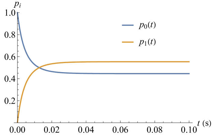
Fig. 2 shows the evolution of and found with the help of Eq. (34). While it may look that the memristor switching is incomplete on average, in fact, the circuit dynamics is a two-time-scale process where the fast initial relaxation (such as the visible one in Fig. 2) transforms into a very slow one occurring on the time scale of (as a consequence of Eq. (3)). Clearly, the fast initial relaxation decelerates with time as the voltage builds up across the capacitor.
The mean switching time for the dynamics in Fig. 2 can be calculated using
| (35) |
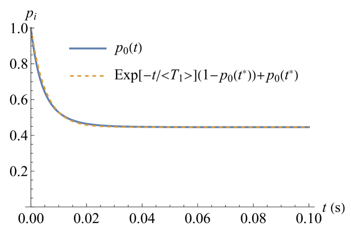
where is the characteristic saturation time for the fast initial dynamics of . Taking s, one can find that ms, which is in perfect agreement with the behavior in Fig. 2. The exponential relaxation with the mean switching time provides an excellent approximation for the initial interval of fast evolution of , see Fig. 3. On long times, the relaxation can be approximated by .
Moreover, by using Eq. (34) one can find in the most interesting parameter region corresponding to the initial interval of fast evolution. This is accomplished employing the asymptotic expansion of the exponential integral function , when . For the time interval , we can omit the second term in the square brackets in Eq. (34) and use the asymptotic expansion for the first one. This leads us to the following expression for the probability of no switching event
| (36) |
For the same parameter values as in Fig. 2, Eq. (36) gives , which is in an excellent agreement with the result obtained numerically from Eq. (34) .
IV Discission
The method used to model the memristor-capacitor circuit above can be straightforwardly extended to other circuits. Consider, for instance, a circuit composed of -state stochastic memristors, capacitors and inductors. In the general case, the simulation of such a circuit requires probability distribution functions of variables and time. Circuits with symmetries may require less functions to represent their states (see Ref. Dowling et al., 2021 for examples). The number of independent reactive variables can be less than . For example, if the external voltage is applied directly across some capacitor, then its charge is not an independent variable.
It is anticipated that the general evolution equation can be written similarly to Eqs. (13) and (14). Introducing the sets of capacitive and inductive variables, and , the evolution equation for a particular state is formulated as
| (37) |
where the memristive switching rates corresponds to the flip of a single memristor and depend on the voltage across the same memristor in a particular circuit configuration. In order to close Eq. (37) we need to express the full derivatives and as functions of by using the Kirchhoff’s circuit laws. If there are no transitions, then the RHS of Eq. (37) turns to zero and this equation coincides with the continuity equation for the probability density as it should be.
In conclusion, we have introduced a powerful analytical approach to model heterogeneous stochastic circuits. A simple example was considered in detail and the recipe to apply the approach to other circuits has been formulated. Compared to the traditional Monte Carlo simulations, the proposed approach can be used to derive analytical expressions describing the circuit dynamics on average.
The data that support the findings of this study are available from the corresponding author upon reasonable request.
References
- Chua and Kang (1976) L. O. Chua and S. M. Kang, Proc. IEEE 64, 209 (1976).
- Kvatinsky et al. (2015) S. Kvatinsky, M. Ramadan, E. G. Friedman, and A. Kolodny, IEEE Transactions on Circuits and Systems II: Express Briefs 62, 786 (2015).
- Pershin et al. (2009) Y. V. Pershin, S. La Fontaine, and M. Di Ventra, Phys. Rev. E 80, 021926 (2009).
- Strachan et al. (2013) J. P. Strachan, A. C. Torrezan, F. Miao, M. D. Pickett, J. J. Yang, W. Yi, G. Medeiros-Ribeiro, and R. S. Williams, IEEE Transactions on Electron Devices 60, 2194 (2013).
- Valov et al. (2011) I. Valov, R. Waser, J. R. Jameson, and M. N. Kozicki, Nanotechnology 22, 254003 (2011).
- Jo et al. (2009) S. H. Jo, K.-H. Kim, and W. Lu, Nano letters 9, 496 (2009).
- Gaba et al. (2013) S. Gaba, P. Sheridan, J. Zhou, S. Choi, and W. Lu, Nanoscale 5, 5872 (2013).
- Gaba et al. (2014) S. Gaba, P. Knag, Z. Zhang, and W. Lu, in 2014 IEEE International Symposium on Circuits and Systems (ISCAS) (IEEE, 2014) pp. 2592–2595.
- Menzel et al. (2014) S. Menzel, I. Valov, R. Waser, B. Wolf, S. Tappertzhofen, and U. Böttger, in 2014 IEEE 6th International Memory Workshop (IMW) (2014) pp. 1–4.
- Naous and Salama (2016) R. Naous and K. N. Salama, in CNNA 2016; 15th International Workshop on Cellular Nanoscale Networks and their Applications (2016) pp. 1–2.
- Dowling et al. (2021) V. J. Dowling, V. A. Slipko, and Y. V. Pershin, Chaos, Solitons & Fractals 142, 110385 (2021).
- Dowling et al. (2020) V. J. Dowling, V. A. Slipko, and Y. V. Pershin, Radioengineering (in press); arXiv:2009.05189 (2020).
- Ntinas et al. (2020) V. Ntinas, A. Rubio, and G. C. Sirakoulis, arXiv:2009.06325 (2020).
- Van Kampen (2007) N. G. Van Kampen, Stochastic Processes in Physics and Chemistry, 3rd ed. (North Holland, 2007).
- Strauss (2007) W. A. Strauss, Partial differential equations: An introduction (John Wiley & Sons, 2007).