Solution methods for the growth of a repeating imperfection in the line of a strut on a nonlinear foundation

Solution methods for the growth of a repeating imperfection in the line of a strut on a nonlinear foundation

Abstract

This paper is a theoretical and numerical study of the uniform growth of a repeating sinusoidal imperfection in the line of a strut on a nonlinear elastic Winkler type foundation. The imperfection is introduced by considering an initially deformed shape which is a sine function with an half wavelength. The restoring force is either a bi-linear or an exponential profile. Periodic solutions of the equilibrium problem are found using three different approaches: a semi-analytical method, an explicit solution of a Galerkin method and a direct numerical resolution. These methods are found in very good agreement and show the existence of a maximum imperfection size which leads to a limit point in the equilibrium curve of the system. The existence of this limit point is very important since it governs the appearance of localization phenomena.

Using the Galerkin method, we then establish an exact formula for this maximum imperfection size and we show that it does not depend on the choice of the restoring force. We also show that this method provides a better estimate with respect to previous publications. The decrease of the maximum compressive force supported by the beam as a function of the imperfection magnitude is also determined. We show that the leading term of the development has a different exponent than in subcritical buckling of elastic systems, and that the exponent values depend on the choice of the restoring force.

url]http://rlagrange.perso.centrale-marseille.fr/visible/Site/

1 Introduction

The subject of beam buckling can be found in several situations in industrial applications. Among the most studied are the thermal track buckling and the buckling of subsea pipelines under the effect of temperature and/or pressure. In the latter case, buckling can appear and in both the vertical and horizontal planes, according to the existing restraints imposed by the environment and the backfill. Numerous authors have studied these two applications due to their high practical importance, and have proposed solution methods to determine buckling loads and post-buckling situations. Along time, the techniques used have progressed, based firstly on analytical analyses and latter on numerical methods mostly derived from finite elements models. Thus, based on some early work by Kerr (1974, 1978) studying the stability of railway tracks subjected to thermal buckling, several authors such as Bournazel (1982); Hobbs (1981, 1984) have proposed solution methods where the equilibrium equations were solved in post-buckling configurations to establish relevant buckling loads. In these works, the soil was supposed rigid, while the external forces acting on the beam was assumed as constant as a dead weight or constant friction force. One of the key features of these theories is the fact that the loss of contact (or movement) induces a loss of global stiffness of the structure which leads to subcritical buckling and infinite buckling loads if no imperfection is assumed. Using slightly different arguments, other models were proposed in Croll (1997) and Maltby and Calladine (1995b). In the latter work, equilibrium equations were obtained by assuming sine deflections in the post-buckling situations and using an approximate Galerkin solution method. This method was compared with numerical solutions in Maltby and Calladine (1995a) and against experimental results in Maltby and Calladine (1995b). Though using an approximate solution method, the approach showed good results with respect to the numerical simulation. In order to improve the earlier methods, numerical models were developed in Ju and Kyriakides (1988); Klever et al. (1990); Leroy and Putot (1992); Yun and Kyriakides (1985) to incorporate for instance additional non linear effects in the models, such as non linear geometric and material models. One of the key aspects of work related to the study of the upheaval buckling is the study of the localization phenomenon, which was suspected early in the pioneering work of Tveergard and Needleman (1980, 1981). This aspect was analyzed through numerical simulations in these first papers and in Hunt and Wadee (1991); Hunt and Blackmore (1996), and through analytical approaches based on a double scale expansion of the equilibrium equations in Potier-Ferry (1987), for a beam resting on an elastic non-linear foundation. Based on these results, the study of the localization phenomenon, was continued by using Galerkin techniques (see Wadee, 2000; Whiting, 1997) using the displacement envelopes obtained through the double-scale expansion of Potier-Ferry (1987). A lot of attention has also been paid to the estimation of the mechanical restraint induced by the soil friction and to the effect of backfill on the pipeline behavior, since the corresponding forces were found to highly influence the mechanical behavior of the pipe. In order to feed the corresponding models, experiments were performed (see Palmer et al., 2003; Schaminee et al., 1990; Trautmann et al., 1985a, b) either through centrifuge testing of small-scale pipeline models or through direct testing of buried full scale pipe sections.

The present paper is an attempt to provide additional solutions for the study of the growth of a repeating imperfection in the line of a strut on a nonlinear foundation. In this work, the foundation is supposed to act through an either bi-linear or exponential regularized friction model relating the interaction line force to the transverse displacement (see section 2). These two kinds of models are indeed found in the above mentioned papers describing the soil-pipe interaction models. In the former case, a solution method (piecewise solution) in section 3 is proposed by explicitly solving the equilibrium equation in the regions where the foundation acts linearly and where the friction force is constant, and by connecting the two solutions by adequate boundary solutions. Alternatively, a Galerkin approach of the same problem is developed in section 3 and leads to an explicit solution of the problem, which is developed for the two regularization models. The piecewise solution and the Galerkin approach are consequently compared together and with numerical solutions of the problem in section 4. The post-buckling problem is then studied through the Galerkin approach which provides precise analytical solutions, focusing on the characteristics of a limit point (see section 5) in the equilibrium curve depending on the magnitude of the initial imperfection.

2 Formulation of the differential equation

Figure 1: Half-wavelength imperfection in the line of a strut resting on an elastic foundation. The imperfection is $W_{0}$, the compressive load is $P$ and the buckling displacement is $W$. Springs have a nonlinear elastic force-displacement relationship $\overline{P}\left(W\right)$.

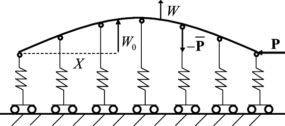
This section formulates the differential equation for the growth of an imperfection in the line of a strut on a nonlinear Winkler-type foundation, see figure 1. The imperfection is introduced by supposing an initially deformed shape $W_{0}$ whose form is

$$W_{0}=A_{0}\sin\left(\frac{\pi}{L}X\right),$$ (1)

with $A_{0}$ the amplitude of the imperfection, $L$ its length and $X$ the longitudinal coordinate. The compressive load is $P$ and the restoring force per unit length is $\overline{P}$. These two forces are assumed to be conservative. The differential equation governing the deflection $W$ may be derived either: directly by equilibration of forces; or from the Principal of Virtual Work; or using an energy formulation. The latter approach is adopted here; the total potential energy at first order being

$$V=\int\limits_{0}^{L}{\left[{\frac{1}{2}EI{W^{{}^{\prime\prime}}}^{2}-P\left({\frac{1}{2}{W^{{}^{\prime}}}^{2}+{{W_{0}}^{{}^{\prime}}}{{W}^{{}^{\prime}}}}\right)-\int\limits_{0}^{W}{\overline{P}\left(t\right)dt}}\right]{\rm{dX}}},$$ (2)

where a prime indicates differentiation with respect to $X$. The first term is the strain energy of bending ($EI$ is the bending stiffness of the strut), the second is the work done by the load $P$ and the remainder is the energy stored in the elastic foundation. Equilibrium is given by stationary values of $V$. In what follows the strut is assumed to be simply supported, such that the conditions at the boundaries are $W\left(0\right)=W\left(L\right)=0$. The calculus of variations on (2) gives, for a virtual displacement $\delta W$ such that $\delta W\left(0\right)=\delta W\left(L\right)=0$

$$\delta V=EI{\left[{\delta W^{{}^{\prime}}W^{{}^{\prime\prime}}}\right]_{0}}^{L}+\int\limits_{0}^{L}{\left[{EI{\rm{}}W^{{}^{\prime\prime\prime\prime}}+P\left({W^{{}^{\prime\prime}}+W_{0}^{{}^{\prime\prime}}}\right)-\overline{P}\left(W\right)}\right]\delta W{\rm{dX}}},$$ (3)

so that the Euler-Lagrange equation and the conditions at the boundaries for a simply supported strut are

$$EIW^{{}^{\prime\prime\prime\prime}}+PW^{{}^{\prime\prime}}-\overline{P}\left(W\right) = -PW_{0}^{{}^{\prime\prime}},$$ (4a)

$$W\left(0\right) = 0,$$ (4b)

$${{W^{\prime\prime}}}\left(0\right) = 0,$$ (4c)

$$W\left(L\right) = 0,$$ (4d)

$${{W^{\prime\prime}}}\left(L\right) = 0.$$ (4e)

In equation (4a), $P$ is the compressive load before buckling. The compressive load after buckling, considering a strut of section $S$, should be written as $N=P-\frac{{ES}}{{2L}}\int\limits_{0}^{L}{\left({W_{,X}}\right)^{2}dX}$, last term of this expression being a geometric shortening which allows for the additional length introduced by the lateral movement. Therefore, $N$ should be used in the equation for equilibrium. However, Tveergard and Needleman (1981) have shown that the buckle will only become unstable if $N(y)$ has a maximum is correct for an isolated half-wave but is not correct for a long strut which contains a sequence of half-waves end-to-end. In such a case the key point is that a localization of the buckling, in which one particular half-wave grows at the expenses of its neighbours, can occur whenever the curve $P(y)$ has a maximum. Under this consideration, and as Maltby and Calladine (1995b) did, we use $P$ instead of $N$ as the load parameter.

2.1 The restoring force

Figure 2: (a) Restoring force. (b) Dimensionless restoring force. Bi-linear profile (solid line), exponential profile (dashed line). Dotted lines: limiting plateau (horizontal line), mobilization (vertical line).

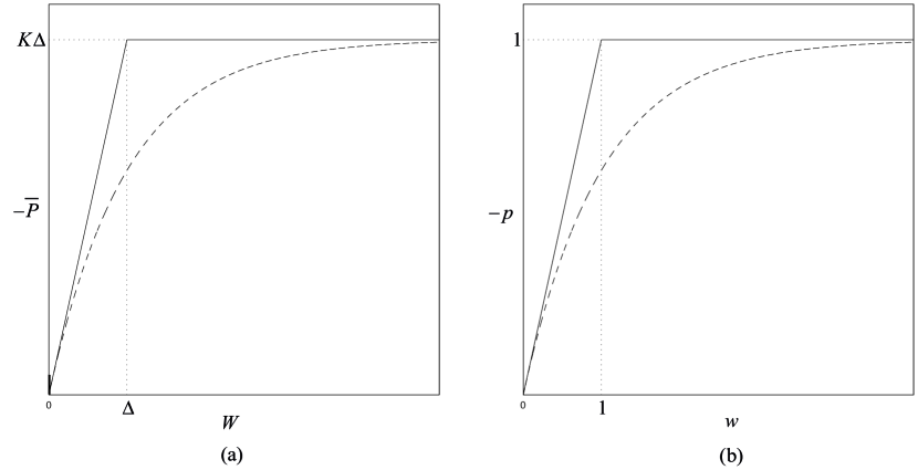
The restoring force per unit length is assumed to be nonlinear and two particular $\overline{P}$ functions are considered. The first one is referred as the bi-linear function and is defined by

$$\overline{P}\left(W\right)=\left\{\begin{array}[]{l}-KW\hskip 28.45274pt{\rm{if}}\hskip 2.84544pt\left|W\right|<\Delta,\\ -K\Delta\hskip 31.2982pt{\rm{if}}\hskip 10.81218ptW>\Delta{\rm{}},\\ K\Delta\hskip 39.83368pt{\rm{if}}\hskip 10.81218ptW<-\Delta,\end{array}\right.$$ (8)

where $K$ is the linear stiffness and $\Delta$ the mobilization. These two constants are positive. The second $\overline{P}$ function considered in this paper is referred as the exponential profile and is defined by

$$\overline{P}\left(W\right)=\left\{\begin{array}[]{l}-K\Delta\left({1-e^{-\frac{W}{\Delta}}}\right)\hskip 24.18501pt{\rm{if}}\hskip 10.81218ptW>0{\rm{}},\\ K\Delta\left({1-e^{\frac{W}{\Delta}}}\right)\hskip 39.83368pt{\rm{if}}\hskip 10.81218ptW<0.\end{array}\right.$$ (11)

The two $\overline{P}$ functions share the same initial slope and limiting force (see figure 2(a)).

2.2 Nondimensionalization

Let’s introduce a characteristic length $L_{char}=\left({\frac{{EI}}{K}}\right)^{\frac{1}{4}}$ and nondimensional quantities

$$l=\frac{{L}}{{L_{char}}},x=\frac{{X}}{{L_{char}}},w=\frac{{W}}{{\Delta}},w_{0}=\frac{{W_{0}}}{{\Delta}},\lambda=\frac{P}{{K{L_{char}}^{2}}},p=\frac{\overline{P}}{{K\Delta}}.$$ (12)

Hence, from (4) the deflection $w$ is solution of the differential problem

$$w^{{}^{\prime\prime\prime\prime}}+\lambda w^{{}^{\prime\prime}}-p\left(w\right) = -\lambda w_{0}^{{}^{\prime\prime}},$$ (13a)

$$w\left(0\right) = 0,$$ (13b)

$${{w^{\prime\prime}}}\left(0\right) = 0,$$ (13c)

$$w\left(l\right) = 0,$$ (13d)

$${{w^{\prime\prime}}}\left(l\right) = 0,$$ (13e)

the dimensionless imperfection being

$$w_{0}=a_{0}\sin\left(\frac{\pi}{l}x\right),$$ (14)

with $a_{0}=\frac{A_{0}}{\Delta}$.

After nondimensionalization, the bi-linear function rewrites

$$p\left(w\right)=\left\{\begin{array}[]{l}-w\hskip 38.41139pt{\rm{if}}\hskip 2.84544pt\left|w\right|<1,\\ -1\hskip 40.68723pt{\rm{if}}\hskip 10.81218ptw>1,\\ 1\hskip 49.79231pt{\rm{if}}\hskip 10.81218ptw<-1,\\ \end{array}\right.$$ (18)

such that the dimensionless mobilization and limiting force equal 1. The nondimensional exponential profile is given by

$$p\left(w\right)=\left\{\begin{array}[]{l}-\left({1-e^{-w}}\right)\hskip 23.61583pt{\rm{if}}\hskip 10.81218ptw>0{\rm{}},\\ {1-e^{w}}\hskip 52.63777pt{\rm{if}}\hskip 10.81218ptw<0.\end{array}\right.$$ (21)

Figure 2(b) shows the evolution of these two dimensionless restoring forces for $w>0$.

3 Theoretical resolution

In this paper, imperfections with dimensionless lengths $l<\sqrt{2}\pi$ are considered. In order to give a practical meaning to this inequation, let’s consider the case of an imperfect railway. The most common rails in France (rail type 50E6) have a weight per meter of about $m=500$ N m^-1, a length from $10$ to $400$ m (length between two joints connection) and a bending stiffness of about $EI=4\times 10^{6}$ N m². Considering a coefficient of friction $\varphi$ between steel and concrete of $0.4$ and a mobilization $\Delta$ from $0.1$ to $1$ mm it comes a linear stiffness $K=\frac{mg\varphi}{\Delta}$ ($g$ being the gravity) from $2\times 10^{5}$ to $2\times 10^{6}$ N m^-2 and a characteristic length $L_{char}$ from $1$ to $2$ m. Therefore $l<\sqrt{2}\pi$ would correspond to a repeating sinusoidal imperfection in the railway whose half-wavelength is no more than $10$ m. In a more general way, $l<\sqrt{2}\pi$ deals with imperfections whose length does not exceed some meters. Therefore the specific calculations described in this paper have been made in the context of a small-scale experimental setup.

For $l<\sqrt{2}\pi$, the first buckling mode predicted by the linear analysis is excited when

$$\lambda=\lambda_{c}=\left({\frac{{\pi}}{l}}\right)^{2}+\left({\frac{{\pi}}{l}}\right)^{-2},$$ (22)

and it has the same shape as the imperfection. In what follows we will also introduce the Euler load $\lambda_{e}$

$$\lambda_{e}=\left({\frac{{\pi}}{l}}\right)^{2},$$ (23)

which is the buckling load of the first mode when the restoring force equals 0.

Two theories are developed to solve the equilibrium problem. The first one, named piecewise solution theory is an exact resolution of the equilibrium problem when the bi-linear restoring force is considered. The second theory is based on a Galerkin method: it leads to an approximate resolution of the equilibrium problem by considering equally the bi-linear or the exponential restoring force. To initiate this method, the deflection shape is assumed to be a sinusoid, as the imperfection. Explicit solutions of the Galerkin equation are obtained without any assumptions.

3.1 Piecewise solution theory

The principle of the piecewise solution theory is to solve (13a) on each piece of the bi-linear function. Then, the solutions are connected thanks to the boundary conditions and assuming the continuity of $w$, $w^{{}^{\prime}}$, $w^{{}^{\prime\prime}}$ and $w^{{}^{\prime\prime\prime}}$ at two connecting points $x_{1}$ and $x_{2}$.

Substituting $p\left(w\right)$ by $-w$ and by $-1$ in (13a) yields respectively

$${{w_{1}^{{}^{\prime\prime\prime\prime}}}}+\lambda{{w_{1}^{{}^{\prime\prime}}}}+w_{1} = -\lambda{w_{0}^{{}^{\prime\prime}}},$$ (24a)

$${{w_{2}^{{}^{\prime\prime\prime\prime}}}}+\lambda{{w_{2}^{{}^{\prime\prime}}}} = -1-\lambda{w_{0}^{{}^{\prime\prime}}}.$$ (24b)

The solutions $w_{1}$ and $w_{2}$ belong to two affine spaces of dimension 4 given by

$$w_{1} = {w_{1}}_{\rm{h}}+{{w_{1}}_{\rm{part}}},$$ (25a)

$$w_{2} = {w_{2}}_{\rm{h}}+{{w_{2}}_{\rm{part}}},$$ (25b)

where ${w_{1}}_{\rm{h}}$ and ${w_{2}}_{\rm{h}}$ satisfy the homogeneous equations

$${{{{w_{1}}_{\rm{h}}}^{{}^{\prime\prime\prime\prime}}}}+\lambda{{{{w_{1}}_{\rm{h}}}^{{}^{\prime\prime}}}}+{w_{1}}_{\rm{h}} = 0,$$ (26a)

$${{{{w_{2}}_{\rm{h}}}^{{}^{\prime\prime\prime\prime}}}}+\lambda{{{{w_{2}}_{\rm{h}}}^{{}^{\prime\prime}}}} = 0.$$ (26b)

Inserting ${w_{1}}_{\rm{h}}=A{\rm{e}}^{r_{1}x}$ and ${w_{2}}_{\rm{h}}=B{\rm{e}}^{r_{2}x}$ in (26) yields two algebraic equations

$$r_{1}^{4}+\lambda{r_{1}}^{2}+1 = 0,$$ (27a)

$$r_{2}^{4}+\lambda{r_{2}}^{2} = 0,$$ (27b)

whose solutions are

$${r_{1}}^{\left(1\right)} = \frac{1}{2}\left[{-2\lambda+2\left({\lambda^{2}-4}\right)^{{1\mathord{\left/{\vphantom{12}}\right.\kern-1.2pt}2}}}\right]^{{1\mathord{\left/{\vphantom{12}}\right.\kern-1.2pt}2}},$$ (28a)

$${r_{1}}^{\left(2\right)} = -\frac{1}{2}\left[{-2\lambda+2\left({\lambda^{2}-4}\right)^{{1\mathord{\left/{\vphantom{12}}\right.\kern-1.2pt}2}}}\right]^{{1\mathord{\left/{\vphantom{12}}\right.\kern-1.2pt}2}},$$ (28b)

$${r_{1}}^{\left(3\right)} = \frac{1}{2}\left[{-2\lambda-2\left({\lambda^{2}-4}\right)^{{1\mathord{\left/{\vphantom{12}}\right.\kern-1.2pt}2}}}\right]^{{1\mathord{\left/{\vphantom{12}}\right.\kern-1.2pt}2}},$$ (28c)

$${r_{1}}^{\left(4\right)} = -\frac{1}{2}\left[{-2\lambda-2\left({\lambda^{2}-4}\right)^{{1\mathord{\left/{\vphantom{12}}\right.\kern-1.2pt}2}}}\right]^{{1\mathord{\left/{\vphantom{12}}\right.\kern-1.2pt}2}},$$ (28d)

and

$$r_{2}=0,\pm\sqrt{\lambda}{\rm{i}}.$$ (29)

Let’s introduce $\alpha_{i}$ and $\omega_{i}$ the real and imaginary parts of ${r_{1}}^{\left(i\right)}$. For $\lambda<2$, the roots $r_{1}$ are complex numbers and the function ${{w_{1}}_{\rm{h}}}$ is

$${{w_{1}}_{\rm{h}}}=A_{1}e^{\alpha_{1}x}\cos\left({\omega_{1}x}\right)+A_{2}e^{\alpha_{2}x}\cos\left({\omega_{2}x}\right)+A_{3}e^{\alpha_{1}x}\sin\left({\omega_{1}x}\right)$$

$$+A_{4}e^{\alpha_{2}x}\sin\left({\omega_{2}x}\right),$$ (30)

with $A_{1}$, $A_{2}$, $A_{3}$ and $A_{4}$ four real constants. For $\lambda=2$, the roots $r_{1}$ are double imaginary numbers (${r_{1}}^{\left(1\right)}={r_{1}}^{\left(3\right)}$ and ${r_{1}}^{\left(2\right)}={r_{1}}^{\left(4\right)}$). The function ${{w_{1}}_{\rm{h}}}$ is

$${{w_{1}}_{\rm{h}}}=\left({A_{1}x+A_{2}}\right)\cos\left(x\right)+\left({A_{3}x+A_{4}}\right)\sin\left(x\right).$$ (31)

For $\lambda>2$, the roots $r_{1}$ are imaginary numbers. The solution ${{w_{1}}_{\rm{h}}}$ is

$${{w_{1}}_{\rm{h}}}=A_{1}\cos\left({\omega_{1}x}\right)+A_{2}\cos\left({\omega_{3}x}\right)+A_{3}\sin\left({\omega_{1}x}\right)+A_{4}\sin\left({\omega_{3}x}\right).$$ (32)

For $\lambda\neq 0$ the function ${{w_{2}}_{\rm{h}}}$ is given by

$${{w_{2}}_{\rm{h}}}=B_{1}+B_{2}x+B_{3}\cos\left({\sqrt{\lambda}x}\right)+B_{4}\sin\left({\sqrt{\lambda}x}\right),$$ (33)

with $B_{1}$, $B_{2}$, $B_{3}$ and $B_{4}$ four real constants.

Since ${{w_{1}}_{\rm{h}}}$ and ${{w_{2}}_{\rm{h}}}$ depend on 4 undetermined constants, these functions will be noted ${{w_{1}}_{\rm{h}}}\left(x,A_{1},A_{2},A_{3},A_{4}\right)$ and ${{w_{2}}_{\rm{h}}}\left(x,B_{1},B_{2},B_{3},B_{4}\right)$.

The functions ${{w_{1}}_{\rm{part}}}$ and ${{w_{2}}_{\rm{part}}}$ appearing in (25a) and (25b) are particular solutions of (24a) and (24b), with $w_{0}$ given by (14). Searching ${{w_{1}}_{\rm{part}}}$ and ${{w_{2}}_{\rm{part}}}$ as ${{w_{1}}_{\rm{part}}}=Aw_{0}$ and ${{w_{2}}_{\rm{part}}}=Cx^{2}+Aw_{0}$, yields

$${{w_{1}}_{\rm{part}}} = \frac{{\lambda}}{{\lambda_{c}-\lambda}}w_{0},$$ (34a)

$${{w_{2}}_{\rm{part}}} = -\frac{1}{\lambda}\frac{{x^{2}}}{2}+\frac{{\lambda}}{{{\lambda_{e}}-\lambda}}w_{0}.$$ (34b)

Finally, the functions $w_{1}$ and $w_{2}$, defined by (25a) and (25b), are

$$w_{1} = {{w_{1}}_{\rm{h}}}\left({x,A_{1},A_{2},A_{3},A_{4}}\right)+\frac{{\lambda}}{{\lambda_{c}-\lambda}}w_{0},$$ (35a)

$$w_{2} = {{w_{2}}_{\rm{h}}}\left({x,B_{1},B_{2},B_{3},B_{4}}\right)-\frac{1}{\lambda}\frac{{x^{2}}}{2}+\frac{{\lambda}}{{\lambda_{e}-\lambda}}w_{0}.$$ (35b)

In what follows, we will introduce the function $w_{3}$ defined as

$$w_{3}={{w_{1}}_{\rm{h}}}\left({x,C_{1},C_{2},C_{3},C_{4}}\right)+\frac{{\lambda}}{{\lambda_{c}-\lambda}}w_{0}.$$ (36)

This function is a solution of (24a), as $w_{1}$, but with 4 different undetermined constants $C_{1}$, $C_{2}$, $C_{3}$ and $C_{4}$.

The aim of the piecewise solution theory is to search for a deflection $w$ solution of (13) by connecting the functions $w_{1}$, $w_{2}$ and $w_{3}$ at two unknown points $x_{1}$ and $x_{2}$ such that

$$w=\left\{\begin{array}[]{l}w_{1}\hskip 38.98013pt{\rm{if}}\hskip 2.84544ptx\in\left[{0,x_{1}}\right[,\\ 1\hskip 44.9554pt{\rm{if}}\hskip 2.84544ptx=x_{1},\\ w_{2}\hskip 38.98013pt{\rm{if}}\hskip 2.84544ptx\in\left]{x_{1},x_{2}}\right[,\\ 1\hskip 44.9554pt{\rm{if}}\hskip 2.84544ptx=x_{2},\\ w_{3}\hskip 38.98013pt{\rm{if}}\hskip 2.84544ptx\in\left]{x_{2},l}\right].\\ \end{array}\right.$$ (37)

With these notations, the boundary conditions (13b), (13c), (13d) and (13e) rewrites

$$w_{1}\left(0\right) = 0,$$ (38a)

$${{w_{1}^{{}^{\prime\prime}}}}\left(0\right) = 0,$$ (38b)

$$w_{3}\left(l\right) = 0,$$ (38c)

$${{w_{3}^{{}^{\prime\prime}}}}\left(l\right) = 0.$$ (38d)

The continuity of the displacement, the tangent, the curvature and the shear at $x_{1}$ yields

$$w_{1}\left(x_{1}\right)-w_{2}\left(x_{1}\right) = 0,$$ (39a)

$${{w_{1}^{{}^{\prime}}}}\left(x_{1}\right)-{{w_{2}^{{}^{\prime}}}}\left(x_{1}\right) = 0,$$ (39b)

$${{w_{1}^{{}^{\prime\prime}}}}\left(x_{1}\right)-{{w_{2}^{{}^{\prime\prime}}}}\left(x_{1}\right) = 0,$$ (39c)

$${{w_{1}^{{}^{\prime\prime\prime}}}}\left(x_{1}\right)-{{w_{2}^{{}^{\prime\prime\prime}}}}\left(x_{1}\right) = 0,$$ (39d)

and at $x_{2}$

$$w_{2}\left(x_{2}\right)-w_{3}\left(x_{2}\right) = 0,$$ (40a)

$${{w_{2}^{{}^{\prime}}}}\left(x_{2}\right)-{{w_{3}^{{}^{\prime}}}}\left(x_{2}\right) = 0,$$ (40b)

$${{w_{2}^{{}^{\prime\prime}}}}\left(x_{2}\right)-{{w_{3}^{{}^{\prime\prime}}}}\left(x_{2}\right) = 0,$$ (40c)

$${{w_{2}^{{}^{\prime\prime\prime}}}}\left(x_{2}\right)-{{w_{3}^{{}^{\prime\prime\prime}}}}\left(x_{2}\right) = 0.$$ (40d)

Equations (38), (39) and (40) lead to a linear system with 12 equations and 12 unknowns (i.e. the amplitudes $A_{i}$, $B_{i}$ and $C_{i}$). A matrix representation of this system is

$${\bf{G}}\left({x_{1},x_{2}}\right){\bf{a}}={\bf{b}}\left({w_{0},x_{1},x_{2}}\right),$$ (41)

with ${\bf{G}}$ a 12 by 12 real matrix and ${\bf{a}}$ the vector of the unknown amplitudes. The vector ${\bf{b}}$ contains the particular solutions ${{w_{1}}_{\rm{part}}}$ and ${{w_{2}}_{\rm{part}}}$ which depend on $w_{0}$, $x_{1}$ and $x_{2}$.

If $\det\left({\bf{G}}\right)\neq 0$ then

$${\bf{a}}\left({w_{0},x_{1},x_{2}}\right)={\bf{G}}^{-1}\left({x_{1},x_{2}}\right){\bf{b}}\left({w_{0},x_{1},x_{2}}\right).$$ (42)

Equation (42) express the amplitudes as functions of $x_{1}$ and $x_{2}$. These two connecting points are obtained by solving the nonlinear system

$$f_{1}\left(w_{0},x_{1},x_{2}\right) = w_{1}\left({x_{1}}\right)-1=0,$$ (43a)

$$f_{2}\left(w_{0},x_{1},x_{2}\right) = w_{2}\left({x_{2}}\right)-1=0.$$ (43b)

The numerical resolution of this system has been carried out with Matlab, using the fzero function. This function tries to find a zero of (43) near $X_{0}$, $X_{0}$ being a vector of length two. Depending on $\lambda$ (43) has 0 or several solutions. For small $\lambda$, the restoring force $p$ remains linear, such that $w=w_{1}$ for any $x\in[0,l]$. Thus, (43) has no solution. For high $\lambda$, the restoring force $p$ is nonlinear: the existence and the uniqueness of a solution for (43) is not trivial. In this paper, we only search for a solution which satisfies $x_{1}\in[0,l/2]$, $x_{2}\in[l/2,l]$ and $x_{2}=l-x_{1}$: the connecting points are symmetric relative to $x=l/2$. This condition is specified adjusting the $X_{0}$ vector used by the fzero function. Typically, $X_{0}=[l/2;l/2]$ is a good candidate to easily find the symmetric connecting points. Once the connecting points are calculated, we determine the amplitudes $A_{i}$, $B_{i}$ and $C_{i}$ thanks to (42), the functions $w_{1}$, $w_{2}$ and $w_{3}$ thanks to (35a), (35b), (36) and finally the deflection $w$ via (37).

3.2 Galerkin method

The Galerkin procedure (see Fox, 1987) may be seen as being derived from (3) by assuming that the modes which go to make up $w$ are given by

$$w=\sum\limits_{i=1}^{n}{y_{i}\phi_{i}},$$ (44)

where each $y_{i}$ is an undetermined amplitude of each shape function $\phi_{i}$. Depending on the form of $w$ in (44), we can perform periodic or localized buckling analysis. For a very long imperfection in the line of a strut on a cubic foundation, Whiting (1997) performed the latter, using the functions predicted by the asymptotical analysis (see Wadee et al., 1997) as test functions. The amplitudes of each shape function are determined numerically using a variable-order variable-step Adams method. In this paper we do not search for localized solutions: we use a unique test function which has the same shape as the imperfection. It means that the deflection $w$ is searched as

$$w=y\sin\left(\frac{\pi}{l}x\right),$$ (45)

with $y>0$.

Inserting $\delta w$ in the dimensionless form of (3) gives

$$\int\limits_{0}^{l}{\sin\left({\frac{\pi}{l}x}\right)\left[{w^{{}^{\prime\prime\prime\prime}}+\lambda\left({w^{{}^{\prime\prime}}+w_{0}^{{}^{\prime\prime}}}\right)-p\left(w\right)}\right]{\rm{dx}}=0}.$$ (46)

Writing the restoring force as $p\left(w\right)=-w-N\left(w\right)$ yields a relation between the load $\lambda$ and the amplitude $y$

$$\lambda=\frac{1}{a_{0}+y}\left[\lambda_{c}y+\frac{Q\left(y\right)}{\lambda_{e}}\right],$$ (47)

with

$$Q\left(y\right)=\frac{2}{l}\int_{0}^{l}\sin\left(\frac{\pi}{l}x\right)N\left(y\sin\left(\frac{\pi}{l}x\right)\right){\rm{dx}}.$$ (48)

The assumption $N\left(y\sin\left(\frac{\pi}{l}x\right)\right)=N\left(y\right)\sin\left(\frac{\pi}{l}x\right)$ introduced by Maltby and Calladine (1995b) yields $N=Q$. Such an assumption will not be introduced in this paper. However, we will see how this assumption affects the result.

Note that since the integrand function in (48) is $l/2$-periodic, the $Q$ function does not change when the deflection is searched as $w=y\sin\left(\frac{n\pi}{l}x\right)$. Then, when the imperfection is $w_{0}=a_{0}\sin\left(\frac{n\pi}{l}x\right)$, the equilibrium paths are still given by (47) with $\lambda_{e}=\left({\frac{{n\pi}}{l}}\right)^{2}$ and $\lambda_{c}=\lambda_{e}+\lambda_{e}^{-1}$.

In practice, the equilibrium paths predicted by the Galerkin method are plotted using (47), varying $y$ and evaluating $\lambda$.

3.2.1 Bi-linear restoring force

Considering the bi-linear restoring force, the $Q$ function rewrites

$$Q\left(y\right)=\frac{2{\rm{H}}\left(y-1\right)}{\pi}\left\{y\left[\arcsin\left(\frac{1}{y}\right)-\frac{\pi}{2}\right]+\left(\frac{y^{2}-1}{y^{2}}\right)^{\frac{1}{2}}\right\},$$ (49)

where ${\rm{H}}$ is the Heaviside function defined by ${\rm{H}}\left({y-1}\right)=0$ if $y<1$ and ${\rm{H}}\left({y-1}\right)=1$ if $y\geq 1$. The proof of this result is reported in A.

3.2.2 Exponential restoring force

Considering the exponential restoring force, the $Q$ function rewrites

$$Q\left(y\right)=2\left[{{\mathop{{\rm I}}\nolimits}_{1}\left(y\right)-{\mathop{{\rm L}}\nolimits}_{1}\left(y\right)}\right]-y,$$ (50)

where ${\rm{I}}_{1}$ and ${\rm{L}}_{1}$ are respectively the modified Bessel and Struve functions of parameter 1. The proof of this result is reported in B.

4 Theoretical and numerical results

In this section, the equilibrium paths predicted by the piecewise solution theory, the Galerkin procedure and a numerical resolution of (13) are compared. We also determine the influence of the restoring force (bi-linear or exponential) on the shape of the equilibrium paths.

4.1 Piecewise solution theory

Figure 3: Equilibrium paths predicted by (a) the piecewise solution theory, (b) the Galerkin method, (c) the numerical resolution of (13), case of a bi-linear restoring force. On each graph, the equilibrium paths are plotted (from top to bottom) for $a_{0}=0$, $a_{0}=0.0238$, $a_{0}=0.595$, $a_{0}=1.19$ and $l=3$. Dotted lines: critical load (upper line), Euler load (lower line), mobilization (vertical line).

Figure 4: Deflection predicted by the piecewise solution theory. (b) is a zoom of (a). Function $w_{1}$ (solid line), function $w_{2}$ (dashed line), function $w_{3}$ (dash-dotted line). The functions $w_{1}$ and $w_{2}$ are connected at $x=x_{1}\approx 0.618$ (first vertical dotted line). The functions $w_{2}$ and $w_{3}$ are connected at $x=x_{2}\approx 2.382$ (second vertical dotted line). The horizontal dotted line represents the mobilization. $l=3$, $a_{0}=0$, $\lambda=1.75$.

The equilibrium paths predicted by the piecewise solution theory are depicted in figure 3(a) for $a_{0}$ from 0 to 1.19. For a small imperfection size, the equilibrium path shows the load increasing at first but then hits a maximum (limit point, or saddle-node bifurcation point) that is below $\lambda_{c}$ (or equals for $a_{0}=0$), and the rest of the path asymptotically decreases to the Euler load when $\max\left(w\right)\rightarrow\infty$. Thus, the system is subcritical. Moreover, the greater the imperfection size, the greater the reduction in the maximum load. Thus the system is imperfection sensitive. For high imperfection sizes, the equilibrium path increases monotically and $\lambda\rightarrow\lambda_{e}<\lambda_{c}$ when $\max\left(w\right)\rightarrow\infty$.

From these observations we infer the existence of a critical amplitude $a_{0c}$ such that

• if $a_{0}>a_{0c}$ then the equilibrium paths do not have a limit point and the equilibrium states are stable,

• if $a_{0}<a_{0c}$ then the equilibrium paths have a limit point $\left(y_{m},\lambda_{m}\right)$. For $y<y_{m}$ (resp. $y>y_{m}$) the equilibrium states are stable (resp. unstable). An unstable equilibrium state is represented in figure 4 by connecting the functions $w_{1}$, $w_{2}$, and $w_{3}$.

The determination of $a_{0c}$ is reported in section 5.

4.2 Galerkin method and numerical results

4.2.1 Bi-linear restoring force

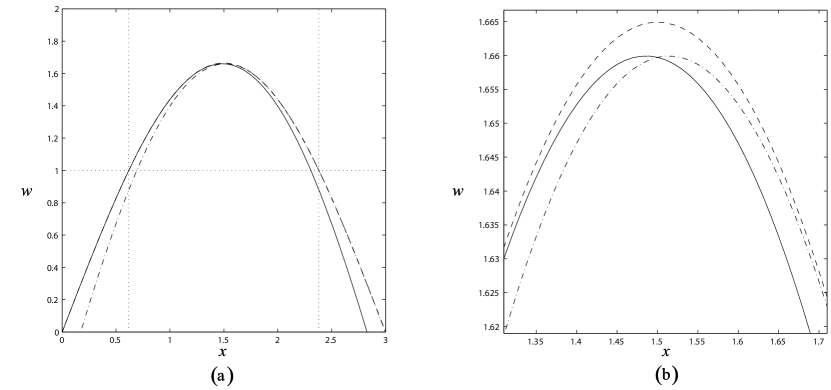
For the bi-linear function, the equilibrium paths predicted by the Galerkin method and those obtained via a numerical resolution of (13), using the ODE45 solver from Matlab (this routine uses a variable step Runge-Kutta method), are represented in figures 3(b) and 3(c). The equilibrium paths are identical to those predicted by the piecewise solution theory (the relative error between the two theories and the numerical resolution being less than $0.1\%$). Since the Galerkin test function and the imperfection have the same shape, in the case of a bi-linear restoring force the deflection is an amplification of the imperfection.

4.2.2 Exponential restoring force

Figure 5: Equilibrium paths predicted by the Galerkin method. Bi-linear restoring force (solid line), exponential restoring force (dashed lines). Galerkin method (upper dashed line), Galerkin method with the Maltby and Calladine (1995b) assumption (lower dashed line). Dotted lines: critical load (upper line), Euler load (lower line), mobilization (vertical line). $l=3$, $a_{0}=0$ (a), $a_{0}=0.0238$ (b), $a_{0}=0.595$ (c), $a_{0}=1.19$ (d).

Figure 6: Equilibrium paths obtained via a numerical resolution of (13), case of an exponential restoring force. Dotted lines: critical load (upper line), Euler load (lower line), mobilization (vertical line). $l=3$, $a_{0}=0$ (a), $a_{0}=0.0238$ (b), $a_{0}=0.595$ (c), $a_{0}=1.19$ (d).

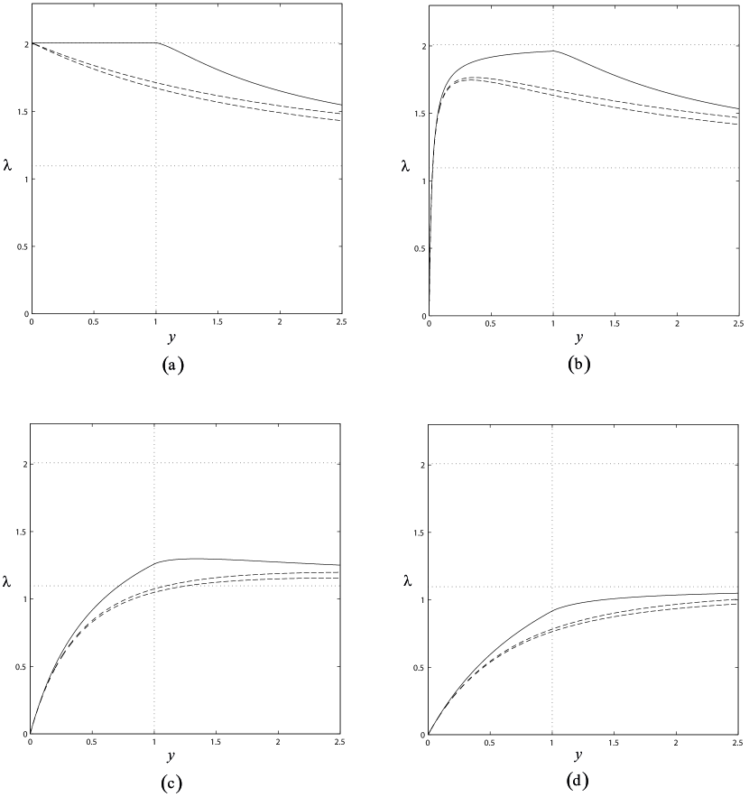
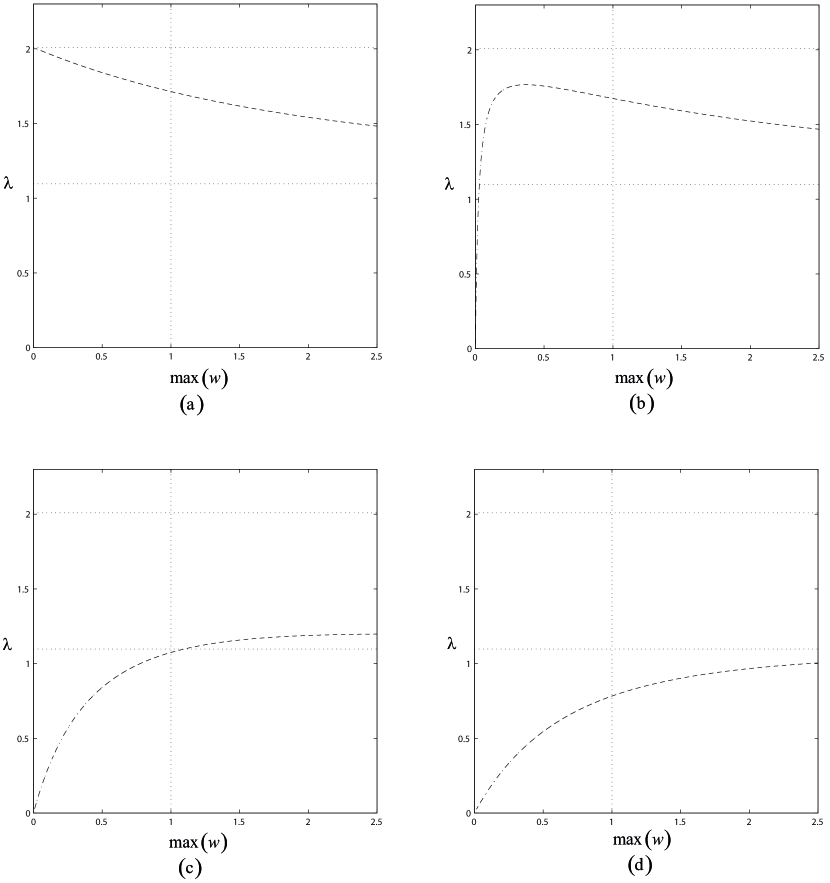
For the exponential profile, the equilibrium paths predicted by the Galerkin method and those obtained via a numerical resolution of (13), are represented in figures 5 and 6. Once again they are identical, thus the deflection $w$ is an amplification of the imperfection. The equilibrium paths predicted by Maltby and Calladine (1995b) have also been reported in figure 5. The assumption introduced by Maltby and Calladine (1995b) (see section 3.2) leads to an underestimation of the load. In section 5 we will show that the existence of a limit point is also affected by this assumption.

In figure 5 the equilibrium paths predicted for a bi-linear restoring force have been reported in order to discuss the influence of the restoring force. It appears that the restoring force (bi-linear or exponential) has no influence on the shape of the equilibrium paths (the variations are preserved, it always exists a limit point for small imperfection sizes, the same asymptotes are recovered). Nevertheless, the equilibrium paths for an exponential profile are below the equilibrium paths for a bi-linear profile. Therefore, the choice of the restoring force has a non negligible influence on the maximal load acceptable by the system. This point is the purpose of the next section.

5 Limit point

Figure 7: Limit point as a function of the amplitude of the imperfection. Bi-linear restoring force (solid line), exponential restoring force (dashed line), exponential restoring force with the assumption introduced by Maltby and Calladine (1995b) (dash-dotted line). Dotted lines: (a) critical amplitudes, (b) critical load (upper line), Euler load (lower line), critical amplitudes (vertical lines). l=3.

Figure 8: Scaling of the limit point. Bi-linear restoring force (solid line), exponential restoring force (dashed line), exponential restoring force with the assumption introduced by Maltby and Calladine (1995b) (dash-dotted line), critical amplitudes (dotted lines). l=3.

Figure 9: Equilibrium paths predicted by the exact Galerkin method (solid curve) and the Galerkin method with the assumption introduced by Maltby and Calladine (1995b) (dashed line). The dotted line corresponds to the Euler load. $a_{0}=0.9$, $l=3$.

A limit point corresponds to a maximum of $\lambda$. Therefore, if it exists, this point $\left(y_{m},\lambda_{m}\right)$ satisfies $\frac{{d\lambda}}{{dy}}\left(y_{m}\right)=0$, that is to say using (47)

$$\left({a_{0}+y_{m}}\right)\frac{{dQ}}{{dy}}\left({y_{m}}\right)-Q\left({y_{m}}\right)=-a_{0}\lambda_{c}\lambda_{e}.$$ (51)

This equation yields $\frac{{Q\left({y_{m}}\right)}}{{\lambda_{e}}}=a_{0}\lambda_{c}-\left({a_{0}+y_{m}}\right){\mathop{{\rm f}}\nolimits}\left({a_{0}}\right)$ with ${\rm{f}}$ a function of $a_{0}$. Inserting this last expression in (47) yields

$$\lambda_{m}=\lambda\left(y_{m}\right)=\lambda_{c}-{\rm{f}}\left(a_{0}\right).$$ (52)

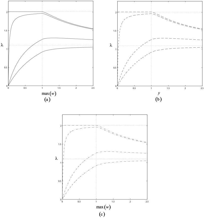
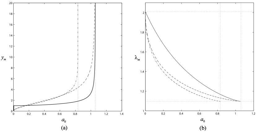
In practice, the coordinates of a limit point are obtained by varying $y_{m}$ and looking for an amplitude $a_{0}$ which satisfies (51). Figure 7(a) represents the evolution of $y_{m}$ as a function of $a_{0}$. For the two restoring forces it appears that $y_{m}$ is an increasing function of $a_{0}$ and diverges for the same critical amplitude. This amplitude is determined by enforcing $y_{m}\rightarrow\infty$ in (51). It yields

$$a_{0c}=\frac{4}{\pi}\lambda_{e}^{-2},$$ (53)

whose dimensional equivalent form is

$$A_{0c}=\frac{4}{\pi}\frac{{L^{4}}}{{\pi^{4}EI}}K\Delta.$$ (54)

This result is of great importance since it governs the appearance of localized solutions, as demonstrated in Tveergard and Needleman (1981). In that paper, they indeed showed the close link between the existence of a limit point in the $\lambda\left(y\right)$ curve and localization, the bifurcation into a localized form occurring a little way beyond this limit point.

Considering the bi-linear restoring force, when $a_{0}\rightarrow 0$, equation (51) has an infinity of solutions $y_{m}$ in $\left]{0,1}\right]$. This observation is coherent with the equilibrium paths depicted in figures 3 since the points lying on the plateau $\lambda=\lambda_{c}$ are a maximum.

Considering the exponential restoring force, $y_{m}\rightarrow 0$ when $a_{0}\rightarrow 0$. This result is coherent with the equilibrium paths depicted in figures 5(a) and 6(a) since $(0,\lambda_{c})$ is a maximum.

Substituting $Q\left(y_{m}\right)$ by $N\left(y_{m}\right)=-y_{m}+1-e^{-y_{m}}$ in (51) (assumption made by Maltby and Calladine (1995b)) and enforcing $y_{m}\rightarrow\infty$ yields

$$a_{0c}=\lambda_{e}^{-2},$$ (55)

whose dimensional equivalent form is

$$A_{0c}=\frac{{L^{4}}}{{\pi^{4}EI}}K\Delta,$$ (56)

which is $\frac{4}{\pi}$ times smaller than the exact prediction (53). This result means that a stable equilibrium (i.e. an equilibrium path without a limit point) predicted with the assumption introduced by Maltby and Calladine (1995b), could in fact be unstable (see figure 9).

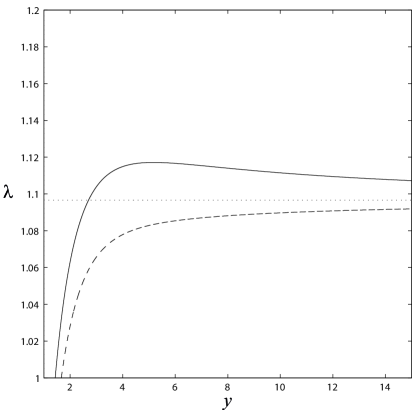
Figure 7(b) represents the evolution of the limit point $\lambda_{m}$ as a function of $a_{0}$. Considering the two restoring forces, the same asymptotes are observed: $\lambda_{m}\rightarrow\lambda_{e}$ when $a_{0}\rightarrow a_{0c}$ and $\lambda_{m}\rightarrow\lambda_{c}$ when $a_{0}\rightarrow 0$. We also observe that the assumption introduced by Maltby and Calladine (1995b) (see section 3.2) leads to an underestimation of the limit load. These observations are coherent with the equilibrium paths depicted in figures 3, 5 and 6.

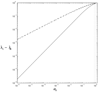
Figure 8 shows the evolution of $\lambda_{c}-\lambda_{m}$ as a function of $a_{0}$, in a logarithmic scale. This picture allows to determine a scaling for the function ${\rm{f}}$ appearing in (52). Considering the bi-linear restoring force, for small amplitudes $a_{0}$, $\lambda_{m}-\lambda_{c}$ scales as

$$\lambda_{m}-\lambda_{c}\sim-a_{0}.$$ (57)

When the exponential restoring force is considered this scaling becomes

$$\lambda_{m}-\lambda_{c}\sim-a_{0}^{{1\mathord{\left/{\vphantom{12}}\right.\kern-1.2pt}2}}.$$ (58)

We observe in figure 8 that the assumption introduced by Maltby and Calladine (1995b) has no influence on this last scaling.

6 Conclusion

In this paper, the growth of a repeating sinusoidal imperfection in the line of a strut on a nonlinear elastic Winkler type foundation is considered. The imperfection is introduced by considering an initially sinusoidal deformed shape with an half wavelength. The imperfection length is chosen such that the buckle mode predicted by the linear theory has the same shape as the imperfection (first buckle mode). The nonlinearities are only due to the restoring force provided by the foundation. This restoring force is expressed as a force-displacement relationship which is either a bi-linear or an exponential function. The equilibrium problem is solved using three different methods. The first one, named piecewise solution theory, is dedicated to the bi-linear profile and leads to an exact resolution of the equilibrium problem. The second one is available whatever the restoring force and is based on a Galerkin procedure. This procedure is initiated with a test function which has the same shape as the imperfection. It yields an explicit relation between the compressive load and the amplitude of the test function. This expression is an exact solution of the Galerkin equation and gives an approximate solution of the equilibrium problem. The last method is a numerical resolution of the equilibrium problem, using the ODE45 solver from Matlab. These three solving methods yield the same results: whatever the restoring force (bi-linear or exponential), the bifurcation is subcritical, the system is imperfection sensitive and the deformed shape is an amplification of the default. Moreover, it exists a critical imperfection size $a_{0c}=\frac{4}{\pi}\lambda_{e}^{-2}$ ($\lambda_{e}$ being the Euler load) which does not depend on the restoring force and such that

• if $a_{0}>a_{0c}$, then the equilibrium path shows the load increasing monotically and remains asymptotic to the Euler load.

• if $a_{0}<a_{0c}$, then the equilibrium path shows the load increasing at first but then hits a limit point and the rest of the path is asymptotic to the Euler load.

This paper provides a better estimate of $a_{0c}$ with respect to previous publications.

For each restoring fore, an approximate mathematical rule is derived relating the imperfection size $a_{0}$ to the corresponding limit load $\lambda_{m}$. Considering the bi-linear profile (resp. the exponential profile) the limit point scales as $\lambda_{m}-\lambda_{c}\sim-a_{0}$ (resp. $\lambda_{m}-\lambda_{c}\sim-a_{0}^{1/2}$), where $\lambda_{c}$ is the critical load issued from the classical linear analysis. Therefore, the scaling of the limit point depends on the regularization method.

In this paper, the restoring force and the compressive load are independent. Nevertheless, in some industrial applications (such as in drilling problems) the restoring force slightly depends on the axial compressive load. Therefore, we are currently carrying out a study with a bi-linear restoring force proportional to the axial load. First results issued from the Galerkin approach indicate that it is necessary to redefine the dimensionless parameters, leading to new scalings for the critical imperfection size and the limit load.

Appendix A Function $Q$, bi-linear restoring force

The aim of this Appendix is to calculate the function $Q$ appearing in (49) when the bi-linear restoring force is considered.

Introduce ${\rm{H}}$ the Heaviside function defined as ${\rm{H}}\left(x\right)=0$ if $x<0$ and ${\rm{H}}\left(x\right)=1$ if $x\geq 0$. The restoring force $p$ rewrites

$$p=-w-\left({{\rm{Sgn}}\left(w\right)-w}\right){\rm{H}}\left({\left|w\right|-1}\right),$$ (59)

where ${\rm{Sgn}}$ is the sign function. Since $p=-w-N\left(w\right)$ it comes

$$N\left(w\right)=\left({{\rm{Sgn}}\left(w\right)-w}\right){\rm{H}}\left({\left|w\right|-1}\right).$$ (60)

For an imperfection with an half-wavelength, it can be assumed that $w>0$. Then, the $Q$ function is (see (48))

$$Q\left(y\right)=-\frac{2}{l}\int_{0}^{l}\left[y\sin\left(\frac{\pi}{l}x\right)-1\right]\sin\left(\frac{\pi}{l}x\right){\rm{H}}\left({y\sin\left(\frac{\pi}{l}x\right)-1}\right){\rm{dx}}.$$ (61)

If $y<1$ then ${y\sin\left({\frac{\pi}{l}x}\right)-1}<0$ so ${\rm{H}}\left({y\sin\left({\frac{\pi}{l}x}\right)-1}\right)=Q=0$. Therefore, the function $Q$ can be written as

$$Q\left(y\right)=-\frac{2{\rm{H}}\left(y-1\right)}{l}\int\limits_{0}^{l}{\left[{y\sin\left({\frac{\pi}{l}x}\right)-1}\right]}\sin\left({\frac{\pi}{l}x}\right){\rm{H}}\left({y\sin\left({\frac{\pi}{l}x}\right)-1}\right){\rm{dx}}.$$ (62)

The change of variable $t=\frac{\pi}{l}x$ gives

$$Q\left(y\right)=-\frac{2}{\pi}{\rm{H}}\left(y-1\right)\int\limits_{0}^{\pi}{\left[{y\sin\left(t\right)-1}\right]}\sin\left(t\right){\rm{H}}\left({y\sin\left(t\right)-1}\right){\rm{dt}}.$$ (63)

The argument of the Heaviside function under the integral sign equals 0 when $\sin\left(t\right)=\frac{1}{y}$, that is to say for $t=t_{1}=\arcsin\left(\frac{1}{y}\right)$ and $t={\pi}-t_{1}$. It comes that the function $Q$ is non zero between $t_{1}$ and ${\pi}-t_{1}$

$$Q\left(y\right)=-\frac{2}{\pi}{\rm{H}}\left(y-1\right)\int\limits_{t_{1}}^{{\pi}-t_{1}}{\left[{y\sin\left(t\right)-1}\right]}\sin\left(t\right){\rm{dt}}.$$ (64)

Finally, this integral yields

$$Q\left(y\right)=\frac{2}{\pi}{\rm{H}}\left({y-1}\right)\left\{{y\left[\arcsin\left({\frac{1}{y}}\right)-\frac{\pi}{2}\right]+\left({\frac{{y^{2}-1}}{{y^{2}}}}\right)^{\frac{1}{2}}}\right\},$$ (65)

and the result from (49) is recovered.

Appendix B Function $Q$, exponential restoring force

The aim of this Appendix is to calculate the function $Q$ appearing in (50) when the exponential restoring force is considered. For this calculus, we recall that the modified Struve and Bessel functions of parameter 1 can be expended as power series

$${\rm{L}}_{1}\left(y\right) = \sum\limits_{p=1}^{+\infty}{\frac{2}{\pi}\frac{{\left({p!}\right)^{2}}}{{\left({2p+1}\right)\left[{\left({2p}\right)!}\right]^{2}}}\left({2y}\right)^{2p}},$$ (66a)

$${\rm{I}}_{1}\left(y\right) = \sum\limits_{p=0}^{+\infty}{\frac{1}{{p!\left({p+1}\right)!}}\left({\frac{y}{2}}\right)^{2p+1}}.$$ (66b)

Substituting the exponential function in (21) by its power series yields

$$p\left(w\right)=-w+\sum_{n=2}^{+\infty}\frac{\left(-1\right)^{n}w^{n}}{n!},$$ (67)

so that

$$N\left(w\right)=\sum_{n=2}^{+\infty}\frac{\left(-1\right)^{n+1}w^{n}}{n!}.$$ (68)

Therefore, (48) gives

$$Q\left(y\right)=\frac{2}{l}\int_{0}^{l}\sum_{n=2}^{+\infty}\frac{\left(-1\right)^{n+1}\sin\left(\frac{\pi}{l}x\right)^{n+1}}{n!}y^{n}{\rm{dx}}.$$ (69)

Inverting the sum and integral signs and introducing the change of variable $t=\frac{\pi}{l}x$ yields

$$Q\left(y\right)=\frac{4}{\pi}\sum_{n=2}^{+\infty}\frac{\left(-1\right)^{n+1}W_{n+1}}{n!}y^{n},$$ (70)

with $W_{n}$ the Wallis integral

$$W_{n}=\int\limits_{0}^{{\pi\mathord{\left/{\vphantom{\pi 2}}\right.\kern-1.2pt}2}}{\sin^{n}\left(x\right){\rm{dx}}}.$$ (71)

The terms $W_{n}$ are classical to calculate. For $n=2p$ and $n=2p+1$ it yields

$$W_{2p} = \frac{{\left({2p}\right)!}}{{2^{2p}\left({p!}\right)^{2}}}\frac{\pi}{2},$$ (72a)

$$W_{2p+1} = \frac{{2^{2p}\left({p!}\right)^{2}}}{{\left({2p+1}\right)!}}.$$ (72b)

Splitting the serie appearing in (70) into odd and even indices gives $Q\left(y\right)=\Sigma_{1}\left(y\right)+\Sigma_{2}\left(y\right)$ with

$$\Sigma_{1}\left(y\right) = -\frac{4}{\pi}\sum\limits_{p=1}^{+\infty}{\frac{{W_{2p+1}}}{{\left({2p}\right)!}}y^{2p}},$$ (73a)

$$\Sigma_{2}\left(y\right) = \frac{4}{\pi}\sum\limits_{p=1}^{+\infty}{\frac{{W_{2\left({p+1}\right)}}}{{\left({2p+1}\right)!}}y^{2p+1}}.$$ (73b)

Inserting (72a) in (73a) yields

$$\Sigma_{1}\left(y\right) = -2\sum\limits_{p=1}^{+\infty}{\frac{2}{\pi}\frac{{\left({p!}\right)^{2}}}{{\left({2p+1}\right)\left[{\left({2p}\right)!}\right]^{2}}}\left({2y}\right)^{2p}},$$ (74a)

$$\Sigma_{2}\left(y\right) = 2\sum\limits_{p=0}^{+\infty}{\frac{1}{{p!\left({p+1}\right)!}}\left({\frac{y}{2}}\right)^{2p+1}}-y.$$ (74b)

Equation (66) gives

$$\Sigma_{1}\left(y\right) = -2{\mathop{{\rm L}}\nolimits}_{1}\left(y\right),$$ (75a)

$$\Sigma_{2}\left(y\right) = 2{\mathop{{\rm I}}\nolimits}_{1}\left(y\right)-y,$$ (75b)

with respectively ${\mathop{{\rm L}}\nolimits}_{1}$ and ${\mathop{{\rm I}}\nolimits}_{1}$ the modified Struve and Bessel functions of parameter 1. Finally

$$Q\left(y\right)=\Sigma_{1}\left(y\right)+\Sigma_{2}\left(y\right)=2\left[{{\mathop{{\rm I}}\nolimits}_{1}\left(y\right)-{\mathop{{\rm L}}\nolimits}_{1}\left(y\right)}\right]-y,$$ (76)

and the result from (50) is recovered.

References

• Bournazel (1982) Bournazel, C., 1982. Vertical buckling of buried pipes. Revue de l’Institut Francais du Pétrole. 37(1), 113–122.
• Croll (1997) Croll, J. G. A., 1997. A simplified model of upheaval thermal buckling of subsea pipelines. Thin-Walled Structures. 29, 59–78.
• Fox (1987) Fox, C., 1987. An introduction to the Calculus of Variations. Dover, New York.
• Hobbs (1981) Hobbs, R. E., 1981. Pipeline buckling caused by axial loads. Journal of Constructional Steel Research. 1(2), 2–10.
• Hobbs (1984) Hobbs, R. E., 1984. In-service buckling of heated pipelines. Journal of Transportation Engineering. 110, 175–189.
• Hunt and Blackmore (1996) Hunt, G. W., Blackmore, A., 1996. Principles of localized buckling for a strut on an elastoplastic foundation. Journal of Applied Mechanics. 63(1), 234–239.
• Hunt and Wadee (1991) Hunt, G. W., Wadee, M. K., 1991. Comparative lagrangian formulations for localized buckling. In: Proceedings of The Royal Society of London. Vol. 434 of A Mathematical Physical and Engineering Sciences. pp. 485–502.
• Ju and Kyriakides (1988) Ju, G. T., Kyriakides, S., 1988. Thermal buckling of offshore pipelines. Journal of Offshore Mechanics and Arctic Engineering. 110, 355–364.
• Kerr (1974) Kerr, A. D., 1974. On the stability of the railroad track in the vertical plane. Rail International. 5, 131–142.
• Kerr (1978) Kerr, A. D., 1978. Analysis of thermal track buckling in the lateral plane. Acta Mechanica. 30, 17–50.
• Klever et al. (1990) Klever, F. J., Van Helvoirt, L. C., Sluyterman, A. C., 1990. A dedicated finite-element model for analyzing buckling response of submarine pipelines. In: Proceedings from the Offshore Technology Conference, Houston. pp. 6333–MS.
• Leroy and Putot (1992) Leroy, J. M., Putot, C. J. M., 1992. Behavior of buried flexible pipelines. In: Proceedings from the Offshore Mechanics and Arctic Engineering Conference, Calgary.
• Maltby and Calladine (1995a) Maltby, T. C., Calladine, C. R., 1995a. An investigation into upheaval buckling of buried pipelines: experimental apparatus and some observations. International Journal of Mechanical Sciences. 37, 943–963.
• Maltby and Calladine (1995b) Maltby, T. C., Calladine, C. R., 1995b. An investigation into upheaval buckling of buried pipelines: theory and analysis of experimental observations. International Journal of Mechanical Sciences. 37, 965–983.
• Palmer et al. (2003) Palmer, A. C., White, D. J., Baumgard, A. J., Bolton, M. D., Barefoot, A. J., Finch, M., Powell, T., Faranski, A. S., Baldry, J. A. S., 2003. Uplift resistance of buried submarine pipelines: comparison between centrifuge modeling and full-scale tests. Geotechnique. 53(10), 877–883.
• Potier-Ferry (1987) Potier-Ferry, M., 1987. Foundations of elastic postbuckling theory. In: Lecture notes in Physics. Vol. 288 of Buckling and Post-buckling. pp. 1–82.
• Schaminee et al. (1990) Schaminee, P. E. L., Zorn, N. F., Schotman, G. J. M., 1990. Soil response for pipeline upheaval buckling analyses: full-scale laboratory tests and modelling. In: Proceedings from the Offshore Technology Conference, Houston. pp. 6486–MS.
• Trautmann et al. (1985a) Trautmann, C. H., O’Rourke, T. D., Kulhawy, F. H., 1985a. Lateral force-displacement response of buried pipe. Journal of Geotechnical Engineering. 111(9), 1077–1092.
• Trautmann et al. (1985b) Trautmann, C. H., O’Rourke, T. D., Kulhawy, F. H., 1985b. Uplift force-displacement response of buried pipe. Journal of Geotechnical Engineering. 111(9), 1061–1076.
• Tveergard and Needleman (1980) Tveergard, V., Needleman, A., 1980. On the localization of buckling patterns. Journal of Applied Mechanics. 47(3), 613–619.
• Tveergard and Needleman (1981) Tveergard, V., Needleman, A., 1981. On localized thermal track buckling. International Journal of Mechanical Sciences. 23, 577–587.
• Wadee (2000) Wadee, M. A., 2000. Effects of periodic and localized imperfections on struts on nonlinear foundations and compression sandwich panels. International Journal of Solids and Structures. 37, 1191–1209.
• Wadee et al. (1997) Wadee, M. K., Hunt, G. W., Whiting, A. I. M., 1997. Asymptotic and rayleigh-ritz routes to localized buckling solutions in an elastic instability problem. In: Proceedings of The Royal Society of London. Vol. 453 of A Mathematical Physical and Engineering Sciences. pp. 2085–2107.
• Whiting (1997) Whiting, A. I. M., 1997. A galerkin procedure for localized buckling of a strut on a nonlinear elastic foundation. International Journal of Solids and Structures. 34, 727–739.
• Yun and Kyriakides (1985) Yun, H., Kyriakides, S., 1985. Model for beam-mode buckling of buried pipelines. Journal of Engineering Mechanics. 111(2), 235–253.