Outperforming classical estimation of Post-Newtonian parameters of Earth’s gravitational field using quantum metrology

Abstract

The Hong-Ou-Mandel (HOM) effect is analyzed for photons in a modified Mach-Zehnder setup with two particles experiencing different gravitational potentials, which are later recombined using a beam-splitter. It is found that the HOM effect depends directly on the relativistic time dilation between the arms of the setup. This temporal dilation can be used to estimate the $\gamma$ and $\beta$ parameters of the parameterized post-Newtonian formalism. The uncertainty in the parameters $\gamma$ and $\beta$ are of the order $10^{-8}-10^{-12}$, depending on the quantum state employed.

1 Introduction

General Relativity is a non-linear and metric theory of the gravitational field. The non-linear character of General Relativity has as consequence that very few analytical solutions are known most of which require a high degree of symmetry. In order to compare the predictions of the theory with observational data certain approximations have become invaluable tools. For instance, gravitational waves are often described by solutions to linear approximations of the Einstein equations and do not arise as solutions of the exact equations [1]. Another very useful approximation of General Relativity is the so called post-Newtonian approximation, a method for solving Einstein’s field equations for sources that move slowly compared to the speed of light and that generate weak gravitational fields[2, 3]. This approximation has been intensively employed as a tool to interpret experimental tests of General Relativity and to test alternative metric theories of gravity[4, 5, 6, 7]. Furthermore, this approximation is considered to be sufficiently precise for explaining most solar-system tests that will be carried out in the foreseeable future [3]. The Hong-Ou-Mandel (HOM) effect is a purely quantum effect with no classical counterpart. This effect is observed in an optical arrangement consisting of two photons arriving at a beam-splitter. Classically, the photons should exit the system and be detected at two different ports. Nevertheless, the quantum mechanical description allows for the possibility that the photons emerge at the same output port or at different output ports, depending on whether there are differences in the length of the arms of the array [8]. In the HOM effect we are interested in the measurement of the coincidence probability, that is, the event in which a single photon is detected at each output port. Several applications of HOM effect have been proposed, such as, for instance, measuring the difference of arrival times between photons, that is, a time sensor [9], and applications to quantum information tasks, such as implementation of Bell measurements [10] and the generation of high-dimensional entangled states [11, 12]. Recently, a large improvement on the measurement resolution of arrival times has been reported [9, 13].

Modern studies concerning quantum information techniques in relativistic contexts have been performed by Fuentes et al. [14], where acceleration effects on quantum entanglement in massless two-mode quantum fields were studied. Refinements using massive particles and particles with spin have been carried out [15]. Furthermore, these predictions have already been experimentally confirmed [16]. On the other hand, recent studies focused instead in effects induced by gravity in large-scale optical arrays [17, 18, 19], developing potential applications of quantum entanglement in general relativity such as the estimation of the gravitational acceleration utilizing photons [20], the usage of optical arrays in the post-Newtonian formalism [17, 18, 19], the implementation of Sagnac arrays to measure a rotation parameter of Gödel metric [21, 22], the usage of optical arrays to generate a path-entangled state induced by gravitational time delay in photons [23], and the proposal of a HOM array to study the effect of the gravitational drag [18]. Furthermore, quantum metrology has been considered as a tool for the estimation of gravitational parameters. Kohlrus et al. studied how photons propagating between satellites in a Kerr spacetime can be used to estimate the equatorial velocity and Schwarzschild radius of the gravitational source. In a further study, the same group showed how the rotation in the photon’s polarization induced by the Kerr metric can be utilized to estimate values of Earth’s radius and the distance between satellites [24]. Finally, Kish et al. studied the Kerr rotation parameter by using a Mach-Zehnder interferometer [25].

Motivated by studies of quantum metrology applied in estimation of spacetime parameters and taking into account the need for enhancing parameter estimation with respect to classical estimations in General Relativity, we study the quantum estimation of post-Newtonian parameters using a HOM array. We show how the HOM effect is produced by a path difference between the arms of the interferometer induced by the gravitational field. This effect depends on the gravitational time dilation between the arrival of photons to the detectors, and the wavepacket dispersion. We use this effect to estimate the arrival times in order to calculate the bounds for the precision of the estimation of the post-Newtonian parameters. In order to compare the quantum and classical bounds for the precision we utilize a scheme which only measures arrival times and we compare it with a scheme that relies on the HOM effect. To improve the estimation using the HOM effect, we consider separable and two-mode squeezing vacuum states. Finally, we compare our results with current values and discuss the implications and improvements of applying quantum metrology to this problem for the first time.

This article is organized as follows: in Sec. 2 we compute the temporal delay in a HOM array. In Sec. 3 we calculate the HOM effect induced by the gravitational time dilation. In Sec. 4 we estimate the post-Newtonian parameters using the HOM array. In Sec. 5 we calculate the uncertainties in the measurement of the parameters. Finally, in Sec. 6 we summarize our results and conclude.

2 Temporal delay in a Hong-Ou-Mandel array

In this section we describe the weak field approximation and the metric utilized to calculate the temporal delays of photons that travel in a Hong-Ou-Mandel array.

The post-Newtonian (PN) formalism is a framework that allows us to describe the effects of the gravitational field using a perturbative expansion, which in its simpler form, depends on the Newtonian gravitational potential. We shall use the following spacetime metric in isotropic coordinates within the PN formalism,

$$ds^{2}=\left(1+2\frac{\phi(x)}{c^{2}}+2\beta\frac{\phi^{2}(x)}{c^{4}}\right)c^{2}dt^{2}-\left(1-2\gamma\frac{\phi(x)}{c^{2}}\right)\delta_{ij}dx^{i}dx^{j},$$ (1)

where $\gamma$ is a constant that parametrizes how much spatial curvature is generated by the gravitating mass, and $\beta$ characterizes the non-lineal contribution to the metric field. Our main goal is to use the HOM effect to determine deviations of both parameters from the values within Einstein’s theory, $\gamma=\beta=1$.

Let us consider a HOM interferometer with light sources located at a height $R$, detectors at $R+\Delta h$ and two paths/arms $(\gamma_{2},\gamma_{1})$, as shown in 1. We use the defining property of photons, that is, the fact they move along light-like curves ($ds^{2}=0$), which implies that the change in temporal coordinates is given by

$$\Delta t = \frac{1}{c}\int dx\left(1+2\frac{\phi}{c^{2}}+2\beta\frac{\phi^{2}}{c^{4}}\right)^{-1/2}\left(1-2\gamma\frac{\phi}{c^{2}}\right)^{1/2}$$ (2)

$$\approx \frac{1}{c}\int dx\left(1+\frac{\phi}{c^{2}}+(\frac{3}{2}-\beta)\frac{\phi^{2}}{c^{4}}\right)\left(1-\gamma\frac{\phi}{c^{2}}-\frac{\gamma^{2}}{2}\frac{\phi^{2}}{c^{4}}\right).$$

Furthermore, the proper length of an arbitrary interval in this metric is given by

$$L = \int dx\left(1-2\gamma\frac{\phi}{c^{2}}\right)^{1/2}$$ (3)

$$\approx \int dx\left(1-\gamma\frac{\phi}{c^{2}}-\frac{\gamma^{2}}{2}\frac{\phi^{2}}{c^{4}}\right).$$

Hence, in the HOM interferometer, the proper length of each arm is

$$L_{\gamma_{1}} \approx \left(1-\gamma\frac{\phi(R)}{c^{2}}-\frac{\gamma^{2}\phi^{2}(R)}{2c^{4}}\right)\Delta x_{\gamma_{1}},$$ (4)

$$L_{\gamma_{2}} \approx \left(1-\gamma\frac{\phi(R+\Delta h)}{c^{2}}-\frac{\gamma^{2}\phi^{2}(R+\Delta h)}{2c^{4}}\right)\Delta x_{\gamma_{1}},$$ (5)

where $\Delta x_{\gamma_{1}}$ is the interval of spatial coordinates in the horizontal path.

For each one of the paths $\gamma_{1}$ and $\gamma_{2}$ in the interferometer we have that the interval of temporal coordinates (2) in terms of the proper lengths (4) and (5) become

$$\Delta t_{\gamma_{2}} \approx (1-\frac{\phi(R+\Delta h)}{c^{2}}+(\frac{3}{2}-\beta)\frac{\phi^{2}(R+\Delta h)}{c^{4}})\frac{L_{\gamma_{2}}}{c},$$ (6)

and

$$\Delta t_{\gamma_{1}}\approx(1-\frac{\phi(R)}{c^{2}}+(\frac{3}{2}-\beta)\frac{\phi^{2}(R)}{c^{4}})\frac{L_{\gamma_{2}}}{c}.$$ (7)

In order to observe interference, we demand the condition $\Delta x_{\gamma_{1}}=\Delta x_{\gamma_{2}}$, that is, an array placed on a equipotencial surface is balanced and there is no difference of optical length between the arms of the array. With this constraint, the proper length $L_{\gamma_{1}}$, to second second order in $\phi/c^{2}$, can be written in terms of $L_{\gamma_{2}}$ as

$$\frac{L_{\gamma_{1}}}{L_{\gamma_{2}}} \approx 1+\gamma\frac{g\Delta h}{c^{2}}+2\gamma^{2}\frac{g\Delta h\phi(R)}{c^{4}}.$$ (8)

Then, the proper length of $\gamma_{1}$ becomes

$$L_{\gamma_{1}}\approx\left(1+\gamma\frac{g\Delta h}{c^{2}}+2\gamma^{2}\frac{g\Delta h\phi(R)}{c^{4}}\right)L_{\gamma_{2}}.$$ (9)

Moreover, proper time measured by a clock located at the detectors, which are at the gravitational potential $\phi(R+\Delta h)$, is given by

$$\Delta\tau = \left(1+2\frac{\phi}{c^{2}}+2\beta\frac{\phi^{2}}{c^{4}}\right)^{1/2}\Delta t,$$ (10)

where $\Delta t=\Delta t^{\rm H}_{\gamma_{1}}-\Delta t^{\rm H}_{\gamma_{2}}$ is the difference of temporal coordinates between paths $\gamma_{1}$ and $\gamma_{2}$. Thus, using Eqs. (6) and (7) we have

$$\Delta\tau = \left((\gamma+1)\frac{g\Delta h}{c^{2}}+2(\gamma^{2}-1+\beta)\frac{\phi(R)g\Delta h}{c^{4}}\right)\frac{L_{\gamma_{2}}}{c}.$$ (11)

This expression can be recast considering the effective area $A=L_{\gamma_{2}}\times\Delta h$ of the interferometer. We obtain the expression

$$\Delta\tau = \left((\gamma+1)+2(\gamma^{2}-1+\beta)\frac{\phi(R)}{c}\right)\frac{Ag}{c^{3}}.$$ (12)

As we can see from Eq. (12), this depends on the PN parameters $\gamma$ and $\beta$, where the parameter $\gamma$ is only present to first order in the the gravitational potential and we have contributions of $\gamma$ and $\beta$ to second order in the gravitational potential. According to Eq. (12), given a measurement of the temporal delay $\Delta\tau$ the considered PN parameters are not independent.

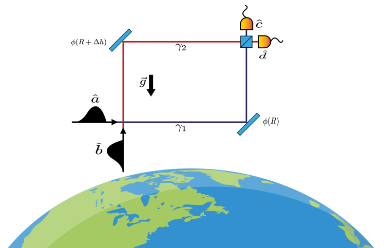
Figure 1: HOM interferometer: two photons are injected to the array. Each photon follows different paths. Each photon experiences a different gravitational potential, for photons moving through horizontal part of path $\gamma_{1}$ experience a gravitational potential $\phi(R)$, and for photons moving along horizontal part of path $\gamma_{2}$ experience a potential $\phi(R+\Delta h)$. Finally photons are recombined at the beam-splitter localized at that potential. The temporal delay in the arrival time of photon is measured by a clock localized besides the detectors.

3 HOM effect induced by gravitational time dilation

Gravitational fields shift the phase of quantum states [17]. This shift is accumulated through different paths of the interferometer and is the source of interference in our system. To calculate the probability of detection in the interferometer we incorporate the effect of gravity by using a unitary operator $U(\varphi)$, where $\varphi$ is the phase. As we know, if we are working in regime where quantum gravity effects are not relevant [26], the propagation of an electromagnetic field is described by the classical wave equations on a curved background. The usual approach consists in describing the propagation of an electromagnetic wave by means of geometric optics [27]. In this approximation, the phase of the vector potential satisfies the eikonal equation, which corresponds to the Hamilton-Jacobi equation for massless particles. In the case of an interferometric experiment, and in a static spacetime, the gravitationally induced phase shift is given by $\Delta\Psi=\bar{\omega}\Delta t$, where $\bar{\omega}$ is the frequency measured by an observer at the infinity and $\Delta t$ is the interval of difference of temporal coordinate between paths of the array. The phase shift can be recast, considering the frequency $\omega$ and the proper time $\Delta\tau$ measured by an observer experiencing a specific gravitation potential, as $\Delta\Psi=\omega\Delta\tau$, with $\omega=\bar{\omega}/\sqrt{g_{00}}$ and $\Delta\tau=\sqrt{g_{00}}$.

3.1 Two-photon separable state

Let us consider an initial two-photon wave packet of the form

$$\ket{\Psi}_{\rm in}=\int d\omega_{1}\phi(\omega_{1})\hat{v}^{\dagger}(\omega_{1})\int d\omega_{2}\phi(\omega_{2})\hat{u}^{\dagger}(\omega_{2})\ket{0}_{12},$$ (13)

where $\hat{v}^{\dagger}$ creates a photon with frequency $\omega_{1}$, and $\hat{u}^{\dagger}$ creates a photon with frequency $\omega_{2}$. The state that describes the photons after the phase shift produced by the gravitational field and the recombination produced by the beam-splitter is

$$\ket{\Psi}_{\rm out} = \frac{1}{2}\iint f(\omega_{1},\omega_{2})e^{-i(\omega_{1}\Delta\tau_{\gamma_{1}}+\omega_{2}\Delta\tau_{\gamma_{2}}+\phi)}\left[ia^{\dagger}(\omega_{1})+b^{\dagger}(\omega_{1})\right]\left[a^{\dagger}(\omega_{1})+ib^{\dagger}(\omega_{1})\right]|0\rangle_{12},$$

where $a,a^{\dagger},b$ and $b^{\dagger}$ are creation and annihilation operators of modes at the output ports of the beam-splitter.

Hence, using Born’s rule, the probability of simultaneous detection is given by

$$p_{cd} = \frac{1}{4}\iint d\omega_{1}d\omega_{2}|\phi(\omega_{1},\omega_{2})|^{2}\left[2-e^{i\left(\omega_{1}-\omega_{2}\right)\tau_{\gamma_{2}}}e^{-i\left(\omega_{1}-\omega_{2}\right)\tau_{\gamma_{1}}}-e^{-i\left(\omega_{1}-\omega_{2}\right)\tau_{\gamma_{2}}}e^{i\left(\omega_{1}-\omega_{2}\right)\tau_{\gamma_{1}}}\right].$$

If the photons have Gaussian frequency distributions, with possibly different spectral distributions $\sigma_{1}$ and $\sigma_{2}$ and mean frequencies $\omega_{1}$ and $\omega_{2}$, the detection probability becomes

$$p_{cd} = \frac{1}{2}\left(1-\cos((\omega_{1}-\omega_{2})\Delta\tau)e^{-\frac{\Delta\tau(\sigma^{2}_{1}+\sigma^{2}_{2})}{4}}\right),$$ (16)

where $\Delta\tau$ is the difference of arrival time measured by a clock placed at the detectors. In the case of photons with the same spectral distributions $\sigma_{1}=\sigma_{2}=\sigma$ and equal mean frequencies $\omega_{1}=\omega_{2}$, the probability of coincidence detection Eq.  (16) becomes

$$p_{cd} = \left(1-e^{-\sigma^{2}\Delta\tau^{2}/2}\right)/2.$$ (17)

According to Eq. (16) the coincidence detection probability decreases exponentially as the temporal delay between photons increases. Moreover, the coincidence detection probability also exhibits an harmonic oscillation given by a cosine function, which depends on the temporal delay times the difference between the mean frequency of the photons. This last feature vanishes if we have twin photons with the same frequency, and only the exponential decrease of the probability is present, according to Eq.  (17). The HOM effect is produced here by the gravitational time dilation, even if both arms have the same proper lengths. If we consider the array placed on a gravitational equipotential surface, there is no difference of proper time, both arms have the same proper length and consequently the coincidence detection probability given by Eq.  (17) vanishes.

Fig. 2 shows behavior of the coincidence detection probability according to Eq. (17) for different values of the parameters $\beta$ and $\gamma$. The range of values for $\gamma$ and $\beta$ is selected between 0.8 and 1.2 in order to visualize the sensitivity of the HOM array to small deviations of these parameters with respect to prediction of General Relativity. In Fig. 3 we plot different values of the parameters $\gamma$ and $\beta$ in terms of the effective area of the HOM interferometer, considering small deviations of actual values of the PN parameters [3]. As is apparent from this figure, the coincidence detection probability of Eq. (17) has nearly the same variation for each value of $\gamma$ and $\beta$ in the case of both parameter with the same values.

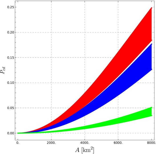
Figure 2: Probability of detection in coincidence for HOM interferometer according to Eq. (17) for different values of $\gamma$ and $\beta$ in the interval $[0.8,1.2]$ and different wavelength width. For each color, upper line represents $\beta=\gamma=1.2$ and mean wavelength $\lambda=3.3\;[\rm\mu m]$, and lower line $\beta=\gamma=0.8$. Red lines $\delta\lambda=0.370\;[\mu m]$, blue lines $\delta\lambda=0.296\;[\mu m]$ and green lines $\delta\lambda=0.148\;[\mu m]$ .

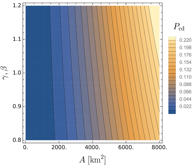
Figure 3: Contour plot for the probability of detection in coincidence for HOM interferometer according to Eq. (17) in terms of different values of $\gamma$ and $\beta$ in the interval $[0.8,1.2]$ and the area $A=L_{\gamma_{2}}\times\Delta h$. The mean wavelength is $\lambda=3.3\;[\rm\mu m]$, and $\delta\lambda=0.370\;[\mu m]$.

To take advantage of the HOM effect, we measure the coincidence detection probability given by the operator

$$\hat{S} = \int d\omega a^{\dagger}(\omega)|0\rangle\langle 0|a(\omega)\otimes\int d\omega b^{\dagger}(\omega)|0\rangle\langle 0|b(\omega).$$ (18)

This is such that,

$$\langle\hat{S}^{2}\rangle=\langle\hat{S}\rangle.$$ (19)

Therefore,

$$\langle\hat{S}\rangle = \frac{1}{2}\left(1-e^{-\sigma^{2}\Delta\tau^{2}/2}\right),$$ (20)

and

$$\langle(\Delta\hat{S})^{2}\rangle = \frac{1}{4}\left(1-e^{-\sigma^{2}\Delta\tau^{2}}\right).$$ (21)

Considering Eqs. (20) and (21) we can calculate the root mean square of the coincidence operator in Eq. (18), where as the elapsed proper time increases, the dispersion present in the observable increases. It is interesting to note that considering Eq. (20) we can obtain an estimation of the temporal delay $\Delta\tau$ through the mean value of the coincidence operator $\hat{S}$.

3.2 Two-mode squeezed-vacuum state

Let us assume that the HOM array is fed a two-mode squeezed-vacuum state, which in the Fock basis is given by

$$|\zeta\rangle = \frac{1}{\cosh(r)}\sum_{n=0}^{\infty}(-1)^{n}e^{in\theta}\left(\tanh(r)\right)^{n}|n,n\rangle.$$ (22)

Here, $\theta$ is a controllable phase for the squeezed vacuum, $r$ is the squeezing parameter of the two-mode squeezer, and $n$ labels Fock states. The probability of detection (for further details see appendix A) of the two photons in coincidence is given by $p_{\rm cd}=\operatorname{Tr}\left(\rho_{\rm squeezing}\hat{S}\right)$, where the operator $\hat{S}$ is given by Eq. (18) and $\rho_{\rm squeezing}=|\zeta\rangle\langle\zeta|$. The probability of coincidence detection in the case of different frequencies, that is, $\omega_{1}\neq\omega_{2}$, becomes

$$\langle S\rangle = \frac{1}{2}\left(\frac{\tanh(r)}{\cosh(r)}\right)^{2}\left(1-\cos((\omega_{1}-\omega_{2})\Delta\tau)e^{-\frac{\Delta\tau(\sigma^{2}_{1}+\sigma^{2}_{2})}{4}}\right).$$ (23)

If the mean frequencies of the Gaussian wave packets are equal, then we obtain

$$\langle S\rangle = \frac{1}{2}\left(\frac{\tanh(r)}{\cosh(r)}\right)^{2}\left(1-\exp\left(-\sigma^{2}\Delta\tau^{2}/2\right)\right).$$ (24)

We can recast Eqs. (23) and (24) considering Eqs. (16) and (17), respectively. In this case, we finally have that the expectation value is given by

$$\langle S\rangle = \left(\frac{\tanh(r)}{\cosh(r)}\right)^{2}P_{cd}.$$ (25)

Thus, the coincidence detection probability of two-mode squeezed-vacuum state is equal to the coincidence detection probability for a two-photo state times a function that depends on the squeezing parameter $r$. In the limit where $r\rightarrow 0$, that is, the squeezing parameter vanishes, the coincidence detection probabilities Eqs. (24) and (23) become Eqs. (17) and (16), respectively.

4 Estimation of $\gamma$ and $\beta$ parameters

4.1 Parameter estimation by an external clock

Considering the temporal delay given by Eq. (11) we use a quantum protocol to obtain an estimate of the parameters $\gamma$ and $\beta$. We consider two different arrival times, for each one we set the HOM interferometer with the lower arm experiencing a gravitational potential $\phi(R_{i})$, with $i=1,2$, and the upper arm experiencing the potential $\phi(R_{i}+\Delta h)$ such that the difference of gravitational potential between each arm (for both interferometers) is (at first order) $g\Delta h$ and each upper arm of the different arrays has a proper length $L_{\gamma_{2}}$ and $L_{\gamma^{\prime}_{2}}$, respectively. A classical approach consists in measuring the time delay of a light wave-packet in the HOM interferometer, but a quantum approach would be based on measuring the difference of proper time through the probability of detection in the HOM array. Having an estimate of the temporal delays in each array, we solve the following system of equations

$$\Delta\tau_{1} = \left((\gamma+1)\frac{g\Delta h}{c^{2}}+2(\gamma^{2}-1+\beta)\frac{\phi(R_{1})g\Delta h}{c^{4}}\right)\frac{L_{\gamma_{2}}}{c},$$ (26)

$$\Delta\tau_{2} = \left((\gamma+1)\frac{g\Delta h}{c^{2}}+2(\gamma^{2}-1+\beta)\frac{\phi(R_{2})g\Delta h}{c^{4}}\right)\frac{L_{\gamma^{\prime}_{2}}}{c}.$$ (27)

Where $\Delta\tau_{1}$ and $\Delta\tau_{2}$ are the differences of arrival time between each configuration of the array, respectively. $\phi(R_{1})$ and $\phi(R_{2})$ are the gravitational potential that is experimented by the lower path of each array, and $\Delta h$ is the difference of spatial coordinate in the z direction (see Fig. (4)). Solving for $\gamma$ and $\beta$, we obtain the following solutions

$$\gamma = \frac{c^{3}\left(L_{\gamma_{2}}\Delta\tau_{2}\phi(R_{1})-L_{\gamma^{\prime}_{2}}\Delta\tau_{1}\phi(R_{2})\right)}{gL_{\gamma_{2}}L_{\gamma^{\prime}_{2}}\Delta h\left(\phi(R_{1})-\phi(R_{2})\right)}-1,$$ (28)

and

$$\beta = \frac{2c^{3}\left(L_{\gamma_{2}}\Delta\tau_{2}\phi(R_{1})-L_{\gamma^{\prime}_{2}}\Delta\tau_{1}\phi(R_{2})\right)}{L_{\gamma_{2}}L_{\gamma^{\prime}_{2}}g\Delta h\left(\phi(R_{1})-\phi(R_{2})\right)}+\frac{c^{5}\left(L_{\gamma^{\prime}_{2}}\Delta\tau_{1}-L_{\gamma_{2}}\Delta\tau_{2}\right)}{2L_{\gamma_{2}}L_{\gamma^{\prime}_{2}}g\Delta h\left(\phi(R_{1})-\phi(R_{2})\right)}$$ (29)

$$-\frac{c^{6}\left(L_{\gamma_{2}}\Delta\tau_{2}\phi(R_{1})-L_{\gamma^{\prime}_{2}}\Delta\tau_{1}\phi(R_{2})\right)^{2}}{L^{2}_{\gamma_{2}}L^{2}_{\gamma^{\prime}_{2}}g^{2}\Delta h^{2}_{1}\left(\phi(R_{1})-\phi(R_{2})\right)^{2}}.$$

In terms of the areas $A_{1}$ and $A_{2}$ of each array the parameters $\gamma$ and $\beta$ become

$$\gamma = \frac{c^{3}\left(A_{1}\Delta\tau_{2}\phi(R_{1})-A_{2}\Delta\tau_{1}\phi(R_{2})\right)}{gA_{1}A_{2}(\phi(R_{1})-\phi(R_{2}))}-1,$$ (30)

$$\beta = \frac{2c^{3}\left(A_{1}\Delta\tau_{2}\phi(R_{1})-A_{2}\Delta\tau_{1}\phi(R_{2})\right)}{A_{1}A_{2}g(\phi(R_{1})-\phi(R_{2}))}+\frac{c^{5}\left(A_{2}\Delta\tau_{1}-A_{1}\Delta\tau_{2}\right)}{2A_{1}A_{2}(\phi(R_{1})-\phi(R_{2}))}$$ (31)

$$-\frac{c^{6}\left(A_{1}\Delta\tau_{2}\phi(R_{1})-A_{2}\Delta\tau_{1}\phi(R_{2})\right)^{2}}{A^{2}_{1}A^{2}_{2}(\phi(R_{1})-\phi(R_{2}))^{2}}.$$

As we can see in the expressions for $\gamma$ and $\beta$, the $\beta$ parameter can be recast in terms of $\gamma$. Thereby, $\beta$ as given by Eq. (31) becomes

$$\beta = \frac{c^{5}\left(A_{2}\Delta\tau_{1}-A_{1}\Delta\tau_{2}\right)}{2A_{1}A_{2}(\phi(R_{1})-\phi(R_{2}))}+2\left(\gamma+1\right)-\left(\gamma+1\right)^{2}.$$ (32)

Consequently, our estimates of $\gamma$ and $\beta$ are dependent, because they arise from an estimate of the same observable, which in our case is the elapsed proper time $\Delta\tau$ of Eq. (12).

4.2 Parameter estimation employing a two-photon separable state

A second way to obtain $\gamma$ and $\beta$ is a slight deviation from the previous one. Instead of considering the time delays of each interferometer (measured with an external clock), we obtain the temporal delay from the probability of detection in the HOM array. Consider the probability of detection in coincidence of Eq. (17), from this probability the time delay (in case of a Gaussian wave-packet) is

$$\Delta\tau_{\rm sep}=\pm\frac{\sqrt{2}}{\sigma}\sqrt{\ln\left(\frac{1}{1-2\langle S\rangle}\right)},$$ (33)

where $\langle S\rangle$ is the expectation value of the coincidence observable (see Eq. 20), and $\sigma$ is the dispersion of the photons. Replacing Eq. (33) for each HOM interferometer in (28) and (29) we obtain

$$\gamma = -1+\frac{c^{3}\Delta h}{gL_{\gamma_{2}}L_{\gamma^{\prime}_{2}}\Delta h^{2}\left(\phi(R_{2})-\phi(R_{1})\right)}$$

$$\times\left(\frac{L_{\gamma^{\prime}_{2}}\phi(R_{1})}{\sigma_{1}}\sqrt{\ln\left(\frac{1}{1-2\langle S_{1}\rangle}\right)}-\frac{L_{\gamma_{2}}\phi(R_{2})}{\sigma_{2}}\sqrt{\ln\left(\frac{1}{1-2\langle S_{2}\rangle}\right)}\right),$$

where $\sigma_{1}$, and $\sigma_{2}$ are the spectral width of the photons employed in the first and second configuration, respectively. $\langle S_{1}\rangle$ and $\langle S_{2}\rangle$ are the expectation values of the coincidence observable for the first and second configuration, respectively. This expression can be recast as

$$\gamma = -1+\frac{c^{3}\Delta h}{gL_{\gamma_{2}}L_{\gamma^{\prime}_{2}}\Delta h^{2}\left(\phi(R_{2})-\phi(R_{1})\right)}$$

$$\times\left(\frac{L_{\gamma^{\prime}_{2}}\phi(R_{1})}{\sigma_{1}}\ln\left(\frac{1}{1-2\langle S_{1}\rangle}\right)-\frac{L_{\gamma_{2}}\phi(R_{2})}{\sigma_{2}}\ln\left(\frac{1}{1-2\langle S_{2}\rangle}\right)\right).$$

Analogously for $\beta$, we obtain

$$\beta = \frac{c^{3}}{2g^{2}L_{\gamma_{2}}L_{\gamma^{\prime}_{2}}\Delta h^{2}\sigma_{1}\sigma_{2}\left(\phi(R_{1})-\phi(R_{2})\right)^{2}}\left[c^{2}gL_{\gamma_{2}}L_{\gamma^{\prime}_{2}}\Delta h\sigma_{1}\sigma_{2}\left(L_{\gamma^{\prime}_{2}}\sigma_{2}\sqrt{\ln\left(\frac{1}{1-2\langle S_{1}\rangle}\right)}\right.\right.$$ (36)

$$\left.\left.-L_{\gamma_{2}}\sigma_{1}\sqrt{\ln\left(\frac{1}{1-2\langle S_{2}\rangle}\right)}\right)\left(\phi(R_{1})-\phi(R_{2})\right)+4gL_{\gamma_{2}}L_{\gamma^{\prime}_{2}}\Delta h\sigma_{1}\sigma_{2}[\phi(R_{1})-\phi(R_{2})]\right.$$

$$\left.\times\left(L_{\gamma_{2}}\sigma_{1}\sqrt{\ln\left(\frac{1}{1-2\langle S_{1}\rangle}\right)}\phi(R_{1})-L_{\gamma^{\prime}_{2}}\sigma_{2}\sqrt{\ln\left(\frac{1}{1-2\langle S_{2}\rangle}\right)}\phi(R_{2})\right)\right.$$

$$\left.-2c^{3}\left(L_{\gamma_{2}}\sigma_{1}\sqrt{\ln\left(\frac{1}{1-2\langle S_{1}\rangle}\right)}\phi(R_{1})-L_{\gamma^{\prime}_{2}}\sigma_{2}\sqrt{\ln\left(\frac{1}{1-2\langle S_{2}\rangle}\right)}\phi(R_{2})\right)\right].$$

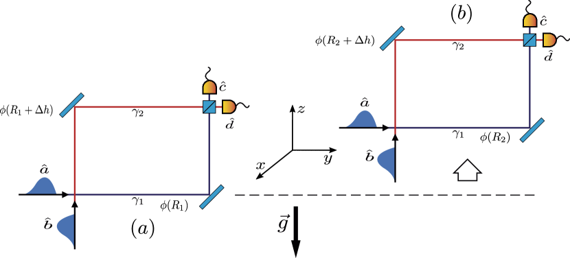
Figure 4: HOM interferometer configuration: in order to obtain the values of the PN parameters $\gamma$ and $\beta$ we measure two different times $\Delta\tau_{1}$ (26) and $\Delta\tau_{2}$ (27) (or the probability of detection in coincidence (17) for each arrival time) for each configuration (a) and (b), respectively. In (a) two photons enter to HOM interferometer, bottom path is in a potential $\phi(R_{1})$ and the upper path in $\phi(R_{1}+\Delta h)$. Both photons are recombined at this potential. For (b) all array is moved a distance such that both photons enter to the array at $\phi(R_{2})$, and finally they are recombined at $\phi(R_{2}+\Delta h)$.

4.3 Parameter estimation employing a two-mode squeezed-vacuum state

In this subsection we employ the probability of detection in coincidence when the HOM array is injected two single-mode vacuum states. Considering the probability of detection given by the Eq. (24), the temporal delay becomes

$$\Delta\tau_{\rm squeezing} = \left(\frac{\sqrt{2}}{\sigma}\right)\sqrt{\ln\left(\frac{\tanh^{2}(r)}{2\langle S\rangle\cosh^{2}(r)-\tanh^{2}(r)}\right)},$$ (37)

where $\langle S\rangle$ is the probability of detection in coincidence. Replacing the temporal delay Eq. (37) the parameter $\gamma$ becomes

$$\gamma = \frac{A_{1}c^{3}\phi(R_{1})\ln\left(\frac{1}{1-2\langle S_{2}\rangle\operatorname{sech}^{4}(r_{2})}\right)-A_{2}c^{3}\phi(R_{2})\ln\left(\frac{1}{1-2\langle S_{1}\rangle\operatorname{sech}^{4}(r_{1})}\right)}{A_{1}A_{2}g\sigma\phi(R_{1})-A_{1}A_{2}g\sigma\phi(R_{2})}-1,$$

where $\langle S_{1}\rangle$ and $\langle S_{2}\rangle$ are the probabilities of detection in coincidence for the first and second configuration of the HOM array, respectively. $r_{1}$ and $r_{2}$ are the expectation values of the squeezing parameter in the first and second configuration, respectively. For the parameter $\beta$ we obtain

$$\beta = -\frac{c^{6}\left(A_{1}\phi(R_{1})\ln\left(\frac{1}{1-2\langle S_{2}\rangle\operatorname{sech}^{4}(R_{2})}\right)-A_{2}\phi(R_{2})\ln\left(\frac{1}{1-2\langle S_{1}\rangle\operatorname{sech}^{4}(R_{1})}\right)\right)^{2}}{A_{1}^{2}A_{2}^{2}g^{2}\sigma^{2}\Delta\phi_{12}^{2}}$$

$$+\frac{A_{2}c^{5}\ln\left(\frac{1}{1-2\langle S_{1}\rangle\operatorname{sech}^{4}(R_{1})}\right)-A_{1}c^{5}\ln\left(\frac{1}{1-2\langle S_{2}\rangle\operatorname{sech}^{4}(R_{2})}\right)}{2A_{1}A_{2}g\sigma\phi(R_{1})-2A_{1}A_{2}g\sigma\phi(R_{2})}$$

$$+\frac{2A_{1}c^{3}\phi(R_{1})\ln\left(\frac{1}{1-2\langle S_{2}\rangle\operatorname{sech}^{4}(R_{2})}\right)-2A_{2}c^{3}\phi(R_{2})\ln\left(\frac{1}{1-2\langle S_{1}\rangle\operatorname{sech}^{4}(R_{1})}\right)}{A_{1}A_{2}g\sigma\phi(R_{1})-A_{1}A_{2}g\sigma\phi(R_{2})}.$$

5 Uncertainties and relative errors of $\gamma$ and $\beta$

In this section, we calculate the uncertainties of the PN parameters $\gamma$ and $\beta$. In the first part we consider errors in the measurement of the arrival time of photons of a classical wave. In the second part we focus on the arrival time obtained from the probability of detection in coincidence, but employing several schemes.

5.1 Errors in the arrival times

To calculate the uncertainty of $\gamma$ and $\beta$ , we consider errors only in the measuring process of the proper time of each HOM interferometer. Moreover the uncertainties of the measurement of the arrival time in each configuration of the HOM array are considered independently, therefore we are assuming that there is no correlation between them. In this case the uncertainty of the parameters $\gamma$ and $\beta$ is given by

$$\delta\epsilon(\Delta\tau_{1},\Delta\tau_{2}) = \sqrt{\left(\frac{\partial\epsilon}{\partial\Delta\tau_{1}}\right)^{2}\delta\Delta^{2}\tau_{1}+\left(\frac{\partial\epsilon}{\partial\Delta\tau_{2}}\right)^{2}\delta\Delta^{2}\tau_{2}},$$ (40)

where $\epsilon=(\gamma,\beta)$ corresponds to each parameter $\gamma$ and $\beta$, $\delta\Delta\tau_{1}$ and $\delta\Delta\tau_{2}$ are the uncertainties on the measurement of the temporal delays $\Delta\tau_{1}$ and $\Delta\tau_{2}$, respectively. Therefore, given the uncertainties $\delta\Delta\tau_{1}$ and $\delta\Delta\tau_{2}$ for the two configurations of the HOM array, the uncertainty in the estimation of $\gamma$ becomes

$$\delta\gamma = \frac{c^{3}}{gL_{\gamma_{2}}L_{\gamma^{\prime}_{2}}\Delta h\left[\phi(R_{1})-\phi(R_{2})\right]}\sqrt{\left(L^{2}_{\gamma_{2}}\delta\Delta\tau^{2}_{1}\phi^{2}(R_{1})+L^{2}_{\gamma^{\prime}_{2}}\delta\Delta\tau^{2}_{1}\phi^{2}(R_{2})\right)}.$$

For the $\beta$ parameter we obtain

$$\delta\beta = \frac{c^{3}}{2g^{2}L^{2}_{\gamma_{2}}L^{2}_{\gamma^{\prime}_{2}}\Delta h^{2}\left[\phi(R_{1})-\phi(R_{2})\right]^{2}}$$

$$\left(L^{2}_{\gamma_{2}}\delta\Delta^{2}\tau_{2}\left[L_{\gamma_{2}}\phi(R_{1})\left(c^{2}gL_{\gamma^{\prime}_{2}}\Delta h+4\phi(R_{1})(c^{3}\Delta\tau_{2}-gL_{\gamma^{\prime}_{2}}\Delta h)\right)\right.\right.$$

$$\left.\left.-L_{\gamma^{\prime}_{2}}\left(c^{2}gL_{\gamma_{2}}\Delta h+4(c^{3}\Delta\tau_{1}-gL_{\gamma_{2}}\Delta h)\phi(R_{1})\right)\phi(R_{2})\right]^{2}\right.$$

$$\left.+L^{2}_{\gamma^{\prime}_{2}}\delta\Delta^{2}\tau_{1}\left[L_{\gamma^{\prime}_{2}}\phi(R_{2})\left((c^{2}gL_{\gamma_{2}}\Delta h+4\phi(R_{2})(c^{3}\Delta\tau_{1}-gL_{\gamma_{2}}\Delta h)\right)\right)\right.$$

$$\left.\left.-L_{\gamma_{2}}\left(c^{2}gL_{\gamma_{2}}\Delta h+4(c^{3}\Delta\tau_{1}-gL_{\gamma_{2}}\Delta h)\phi(R_{2})\right)\phi(R_{1})\right]^{2}\right)^{1/2}.$$

The relative error for the parameter $\gamma$, in terms of the uncertainties $\delta\Delta\tau_{1}$ and $\delta\Delta\tau_{2}$, reads

$$\frac{\delta\gamma}{\gamma} = \frac{\sqrt{c^{6}\left(L^{2}_{\gamma_{2}}\delta^{2}\Delta\tau_{2}\phi^{2}(R_{1})+L^{\prime 2}_{\gamma_{2}}\delta^{2}\Delta\tau_{1}\phi^{2}(R_{2})\right)}}{L^{\prime}_{\gamma_{2}}\left(gL_{\gamma_{2}}\Delta h-c^{3}\Delta\tau_{1}\right)\phi(R_{2})-L_{\gamma_{2}}\left(gL^{\prime}_{\gamma_{2}}\Delta h-c^{3}\Delta\tau_{2}\right)\phi(R_{1})},$$ (43)

or in terms of the proper area

$$\frac{\delta\gamma}{\gamma} = \frac{\sqrt{c^{6}\left(A_{1}^{2}\delta^{2}\Delta\tau_{2}\phi^{2}(R_{1})+A_{2}^{2}\delta^{2}\Delta\tau_{1}\phi^{2}(R_{2})\right)}}{A_{2}\left(gA_{1}-c^{3}\Delta\tau_{1}\right)\phi(R_{2})-A_{1}\left(gA_{2}-c^{3}\Delta\tau_{2}\right)\phi(R_{1})}.$$ (44)

The relative error for the parameter $\beta$ is given by

$$\frac{\delta\beta}{\beta} = -\left(c^{3}\left(2\Delta\tau_{2}L_{\gamma_{2}}^{2}\phi(R_{1})^{2}\left(c^{3}\Delta\tau_{2}-2\Delta hgL^{\prime}_{\gamma_{2}}\right)\right.\right.$$ (45)

$$\left.\left.+L_{\gamma_{2}}L^{\prime}_{\gamma_{2}}\phi(R_{1})\left(4\phi(R_{2})\left(c^{3}(-\Delta\tau_{1})\Delta\tau_{2}+\Delta h\Delta\tau_{2}gL_{\gamma_{2}}+\Delta h\Delta\tau_{1}gL^{\prime}_{\gamma_{2}}\right)\right.\right.\right.$$

$$\left.\left.\left.+c^{2}\Delta hg(\Delta\tau_{2}L_{\gamma_{2}}-\Delta\tau_{1}L^{\prime}_{\gamma_{2}})\right)+L^{\prime}_{\gamma_{2}}\phi(R_{2})\left(2\Delta\tau_{1}L^{\prime}_{\gamma_{2}}\phi(R_{2})\left(c^{3}\Delta\tau_{1}-2\Delta hgL_{\gamma_{2}}\right)\right.\right.\right.$$

$$\left.\left.\left.+c^{2}\Delta hgL_{\gamma_{2}}(\Delta\tau_{1}L^{\prime}_{\gamma_{2}}-\Delta\tau_{2}L_{\gamma_{2}})\right)\right)\right)^{-1}$$

$$\times\left[c^{6}\left(\delta\Delta\tau_{2}^{2}L^{2}_{\gamma_{2}}\left(L_{\gamma_{2}}\phi(R_{1})\left(\phi(R_{1})\left(4c^{3}\Delta\tau_{2}-4\Delta hgL^{\prime}_{\gamma_{2}}\right)+c^{2}\Delta hgL^{\prime}_{\gamma_{2}}\right)\right.\right.\right.$$

$$\left.\left.\left.-L^{\prime}_{\gamma_{2}}\phi(R_{2})\left(\phi(R_{1})\left(4c^{3}\Delta\tau_{1}-4\Delta hgL_{\gamma_{2}}\right)+c^{2}\Delta hgL_{\gamma_{2}}\right)\right)^{2}\right.\right.$$

$$\left.\left.+\delta\Delta\tau_{1}^{2}L^{{}^{\prime}2}_{\gamma_{2}}\left(L^{\prime}_{\gamma_{2}}\phi(R_{2})\left(\phi(R_{2})\left(4c^{3}\Delta\tau_{1}-4\Delta hgL_{\gamma_{2}}\right)+c^{2}\Delta hgL_{\gamma_{2}}\right)\right.\right.\right.$$

$$\left.\left.\left.-L_{\gamma_{2}}\phi(R_{1})\left(\phi(R_{2})\left(4c^{3}\Delta\tau_{2}-4\Delta hgL^{\prime}_{\gamma_{2}}\right)+c^{2}\Delta hgL^{\prime}_{\gamma_{2}}\right)\right)^{2}\right)\right]^{1/2}.$$

This expression can be written in terms of the proper area $A$ of each array as

$$\frac{\delta\beta}{\beta} = -\left(c^{3}\left(2\Delta\tau_{2}A_{1}^{2}\phi(R_{1})^{2}\left(c^{3}\Delta\tau_{2}-2gA_{2}\right)\right.\right.$$ (46)

$$\left.\left.+A_{1}A_{2}\phi(R_{1})\left(4\phi(R_{2})\left(c^{3}(-\Delta\tau_{1})\Delta\tau_{2}+\Delta\tau_{2}gA_{1}+\Delta\tau_{1}gA_{2}\right)+c^{2}g(\Delta\tau_{2}A_{1}-\Delta\tau_{1}A_{2})\right)\right.\right.$$

$$\left.\left.+A_{2}\phi(R_{2})\left(2\Delta\tau_{1}A_{2}\phi(R_{2})\left(c^{3}\Delta\tau_{1}-2gL_{\gamma_{2}}\right)+c^{2}\Delta hgA_{1}(\Delta\tau_{1}A_{2}-\Delta\tau_{2}A_{1})\right)\right)\right)^{-1}$$

$$\times\left[c^{6}\left(\delta\Delta\tau_{2}^{2}A_{1}^{2}\left(A_{1}\phi(R_{1})\left(\phi(R_{1})\left(4c^{3}\Delta\tau_{2}-4gA_{2}\right)+c^{2}gA_{2}\right)\right.\right.\right.$$

$$\left.\left.\left.-A_{2}\phi(R_{2})\left(\phi(R_{1})\left(4c^{3}\Delta\tau_{1}-4gA_{1}\right)+c^{2}gA_{2}\right)\right)^{2}\right.\right.$$

$$\left.\left.+\delta\Delta\tau_{1}^{2}A_{2}^{2}\left(A_{2}\phi(R_{2})\left(\phi(R_{2})\left(4c^{3}\Delta\tau_{1}-4gA_{1}\right)+c^{2}gA_{1}\right)\right.\right.\right.$$

$$\left.\left.\left.-A_{1}\phi(R_{1})\left(\phi(R_{2})\left(4c^{3}\Delta\tau_{2}-4gA_{2}\right)+c^{2}gA_{2}\right)\right)^{2}\right)\right]^{1/2}.$$

Fig. 5 shows the relative error of the parameters $\gamma$ and $\beta$ in accordance with Eqs. (44) and (46), respectively, in terms of the proper area of the first configuration. In the simulation we consider an external clock that measures the arrival times of the photons, which has an uncertainty $\delta\tau_{\rm clock}=10^{-18}\;[s]$, and we consider the same uncertainty for both configurations of the HOM array. In order to simplify the analysis we configure the area of the second array as $A_{2}=\eta\times A_{1}$, with $\eta=1,1/2,1/4,1/8$. As we can see from the figure, the configuration with a lower relative error for the parameters $\gamma$ and $\beta$ is reached with $A_{1}=A_{2}$. In Fig. 6 the uncertainty $\delta\Delta\tau$ necessary to obtain a relative error of the parameters $\gamma$ and $\beta$ of $10^{-5}$ is shown. In this case, the configuration of the HOM array with the higher $\delta\Delta\tau$ corresponds to both interferometers having the same area. From the figure, the uncertainty $\delta\Delta\tau$ for $\gamma$ is $\sim 10^{-22}$, while for $\beta$ it corresponds to $\sim 10^{-31}$. In this case, to obtain the current uncertainties of $\gamma$ and $\beta$ we need a lower error in the arrival times for $\beta$.

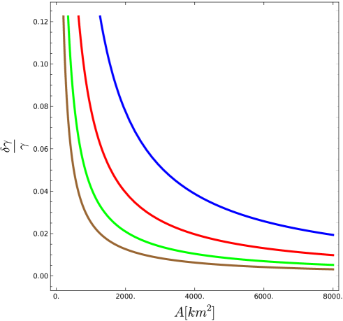
(a)

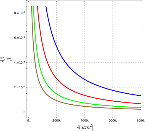
(b)

Figure 5: Relative error of the parameters $\gamma$ and $\beta$, as measured by a external clock placed at the detectors, through Eqs. (26) and  (27) in terms of the area $A=\Delta h\times L_{\gamma_{2}}$ of the array. (a) Relative error for the parameter $\gamma$, and the clock employed has a uncertainty $\delta\tau_{\rm clock}=10^{-18}[\rm s]$. (b) Relative error for the parameter $\beta$. We assume that in both HOM array configuration the clocks have the same uncertainty. $\delta\tau_{\rm clock}=10^{-31}[\rm s]$ . Each array configuration is characterized by an area, $A_{1}$ is used in the measurement of the first time delay and $A_{2}=\eta A_{1}$ is used in the second array, where $\eta$ is a constant. The blue continuous line represents $\eta=1/8$, red continuous line $\eta=1/4$, green continuous line $\eta=1/2$ and brown continuous line $\eta=1$.

(a)

(b)

Figure 6: Uncertainty on the measurement of the temporal delay necessary to obtain the current value in the uncertainty of $\gamma$ and $\beta$, in terms of the area $A=\Delta h\times L_{\gamma_{2}}$ of the array. (a) Uncertainty of $\Delta\tau$ for the parameter $\gamma$. (b) Uncertainty of $\Delta\tau$ for the parameter $\beta$. We assume that in both HOM array configurations the uncertainty in the arrival time is the same. Each array configuration is characterized by an area, $A_{1}$ is used for measuring the first time delay and $A_{2}=\eta A_{1}$ is used in the second array, where $\eta$ is a constant. Blue continuous line represents $\eta=1/8$, red continuous line $\eta=1/4$, green continuous line $\eta=1/2$ and brown continuous line $\eta=1$.

5.2 Errors in the coincidence detection probability

Considering the expectation value of the observable of detection in coincidence for two photons Eq. (20), the uncertainty for the parameter $\gamma$ reads

$$\delta\gamma = \sqrt{\frac{c^{6}\left(\frac{\delta S_{1}^{2}\phi(R_{2})^{2}}{A_{1}^{2}(1-2\langle S_{1}\rangle)^{2}\sigma_{1}^{2}\ln\left(\frac{1}{1-2\langle S_{1}\rangle}\right)}+\frac{\delta S_{2}^{2}\phi(R_{1})^{2}}{A_{2}^{2}(1-2\langle S_{2}\rangle)^{2}\sigma_{2}^{2}\ln\left(\frac{1}{1-2\langle S_{2}\rangle}\right)}\right)}{g^{2}(\Delta\phi_{12})^{2}}},$$ (47)

and for the parameter $\beta$

$$\delta\beta = \frac{1}{2A_{1}^{2}A_{2}^{2}g^{2}\sigma_{1}^{2}\sigma_{2}^{2}(\Delta\phi_{12})^{2}}$$ (48)

$$\times\left(c^{6}\left(\frac{A_{1}^{2}\delta S_{2}^{2}\sigma_{1}^{2}}{(1-2\langle S_{2}\rangle)^{2}\ln\left(\frac{1}{1-2\langle S_{2}\rangle}\right)}\left(A_{1}\sigma_{1}\phi(R_{1})\left(\phi(R_{1})\left(4c^{3}\sqrt{\ln\left(\frac{1}{1-2\langle S_{2}\rangle}\right)}-4A_{2}g\sigma_{2}\right)\right.\right.\right.\right.$$

$$\left.\left.\left.\left.+A_{2}c^{2}g\sigma_{2}\right)-A_{2}\sigma_{2}\phi(R_{2})\left(\phi(R_{1})\left(4c^{3}\sqrt{\ln\left(\frac{1}{1-2\langle S_{1}\rangle}\right)}-4A_{1}g\sigma_{1}\right)+A_{1}c^{2}g\sigma_{1}\right)\right)^{2}\right.\right.$$

$$\left.\left.+\frac{A_{2}^{2}\delta S_{1}^{2}\sigma_{2}^{2}}{(1-2\langle S_{1}\rangle)^{2}\ln\left(\frac{1}{1-2\langle S_{1}\rangle}\right)}\left(A_{2}\sigma_{2}\phi(R_{2})\left(4\phi(R_{2})\left(A_{1}g\sigma_{1}-c^{3}\sqrt{\ln\left(\frac{1}{1-2\langle S_{1}\rangle}\right)}\right)-A_{1}c^{2}g\sigma_{1}\right)\right.\right.\right.$$

$$\left.\left.\left.+A_{1}\sigma_{1}\phi(R_{1})\left(\phi(R_{2})\left(4c^{3}\sqrt{\ln\left(\frac{1}{1-2\langle S_{2}\rangle}\right)}-4A_{2}g\sigma_{2}\right)+A_{2}c^{2}g\sigma_{2}\right)\right)^{2}\right)\right)^{1/2}.$$

Considering the errors Eqs. (47) and (48) together with Eqs. (LABEL:ParamterGamma2) and (36) we can calculate the relative error of the parameters $\gamma$ and $\beta$, we do not show the expression because it is not enlightening. In Fig. 7 we show the relative error of the parameters $\gamma$ and $\beta$. We choose the same configuration of the HOM arrays as in the previous section, as indicated in the figure. The lower relative error for both parameters is reached when both areas are equal. In our simulations we employ states with wavelength $\lambda=0.995\;[\mu m]$ and bandwidth $\delta\lambda=0.034[\mu m]$ employed in current SPDC sources [28], and an error in the measurement of the coincidence operator $\delta S=10^{-18}$. Therefore, the relative error of $\gamma$ and $\beta$ are $\sim 10^{-14}$ and $\sim 10^{-6}$, respectively. Fig.  8 shows the uncertainty $\delta S$ of the measurement of the operator detection in coincidence if we consider the errors currently indicated in the literature, in terms of the effective area of one of the arrays. As in the previous section, considering both configurations of the interferometer with the same proper area we obtain a higher uncertainty $\delta S$. For $\gamma$ the uncertainty $\delta S\sim 10^{-7}$, and for $\beta$ $\delta S\sim 10^{-16}$.

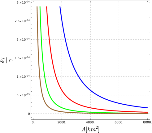
(a)

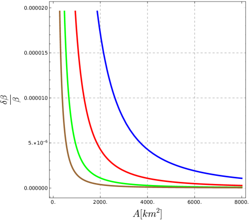
(b)

Figure 7: Relative error of the parameters $\gamma$ and $\beta$ measured through the probability of detection Eq. (17), in terms of the area $A=\Delta h\times L_{\gamma_{2}}$ of the array. (a) Relative error for the parameter $\gamma$. (b) Relative error for the parameter $\beta$. For both simulations the uncertainty in the measure of the probability of detection is $\delta S=10^{-18}$. We assume that in both HOM array configuration the uncertainty in the probability of detection is the same. In the array configuration, $A_{1}$ is the area for the first array configuration, in which the detection of the first time delay is done. The second array has area $A_{2}=\eta A_{1}$, where $\eta$ is a constant. Blue continuous line represents $\eta=1/8$, red continuous line $\eta=1/4$, green continuous line $\eta=1/2$ and brown continuous line $\eta=1$.

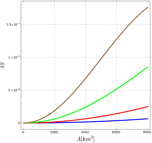
(a)

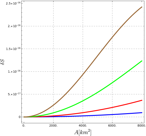
(b)

Figure 8: Uncertainty on the measurement of the coincidence observable S Eq. (18) necessary to obtain the current value in the uncertainty of $\gamma$ and $\beta$, in terms of the area $A=\Delta h\times L_{\gamma_{2}}$ of the array. (a) Uncertainty of S for the parameter $\gamma$. (b) Uncertainty of S for the parameter $\beta$. We assume that in both HOM array configuration the uncertainty in the probability of detection is the same. In the array configuration, $A_{1}$ is the area for the first array configuration, in which the detection of the first time delay is done. The second array has area $A_{2}=\eta A_{1}$, where $\eta$ is a constan. Blue continuous line represents $\eta=1/8$, red continuous line $\eta=1/4$, green continuous line $\eta=1/2$ and brown continuous line $\eta=1$.

5.3 Relative error employing a two-mode squeezed-vacuum state

Here, we calculate the relative error of the parameters $\gamma$ and $\beta$ given in Eqs. (LABEL:gammaSqueezing) and (LABEL:betaSqueezing), respectively. The uncertainty of the parameter $\gamma$ is given by

$$\delta\gamma = \frac{\sqrt{2}c^{3}}{A_{1}A_{2}g\sigma(\phi(R_{1})-\phi(R_{2}))}$$

$$\times\left(A_{1}\phi(R_{1})\ln\left(1-2\langle S_{2}\rangle\left(\tanh^{2}(r_{2})+1\right)^{2}\right)-A_{2}\phi(R_{2})\ln\left(1-2\langle S_{1}\rangle\left(\tanh^{2}(r_{1})+1\right)^{2}\right)\right)-1$$

where $\delta S_{1}$ and $\delta S_{2}$ are the uncertainties on the measurements of the probabilities $\langle S_{1}\rangle$ and $\langle S_{2}\rangle$, respectively. $r_{1}$ and $r_{2}$ are the squeezing parameters employed in the generation of each squeezed single-vacuum state for each configuration of the HOM array, respectively. For the parameter $\beta$ we obtain

$$\delta\beta = \frac{c^{3}}{2A_{1}^{2}A_{2}^{2}g^{2}\sigma^{2}(\phi(R_{1})-\phi(R_{2}))^{2}}$$ (50)

$$\left(-4c^{3}\left(A_{1}\phi(R_{1})\ln\left(1-2\langle S_{2}\rangle\left(\tanh^{2}(r_{2})+1\right)^{2}\right)-A_{2}\phi(R_{2})\ln\left(1-2\langle S_{1}\rangle\left(\tanh^{2}(r_{1})+1\right)^{2}\right)\right)^{2}\right.$$

$$\left.+\sqrt{2}A_{1}A_{2}c^{2}g\sigma(\phi(R_{1})-\phi(R_{2}))\left(A_{2}\ln\left(1-2\langle S_{1}\rangle\left(\tanh^{2}(r_{1})+1\right)^{2}\right)\right.\right.$$

$$\left.\left.-A_{1}\ln\left(1-2\langle S_{2}\rangle\left(\tanh^{2}(r_{2})+1\right)^{2}\right)\right)\right.$$

$$\left.+4\sqrt{2}A_{1}A_{2}g\sigma(\phi(R_{1})-\phi(R_{2}))\left(A_{1}\phi(R_{1})\ln\left(1-2\langle S_{2}\rangle\left(\tanh^{2}(r_{2})+1\right)^{2}\right)\right.\right.$$

$$\left.\left.-\phi(R_{2})\ln\left(1-2\langle S_{1}\rangle\left(\tanh^{2}(r_{1})+1\right)^{2}\right)\right)\right).$$

The relative error of the parameter $\gamma$ is obtained through the coefficient between Eqs. (LABEL:Errorgammasqz) and (LABEL:gammaSqueezing). Analogously, $\beta$ is given by comparing Eqs. (50) and (LABEL:betaSqueezing). Fig. 9 shows the relative error for the parameters $\gamma$ and $\beta$ in terms of the effective area of the HOM array, considering an interval of the squeezing parameter $r$ in the interval $\left[1,2\right]$ and with an uncertainty $\delta S=10^{-13}$. Moreover, we consider that in both configurations of the array, the squeezing parameters are equal to $r$. In this sense, we obtain a lower relative error for both parameters when $r=1$, this is, increasing the squeezing parameter does not reduce relative errors. In this case we have employed the same analysis as before i.e. the area of the second configuration of the array is given by $A_{2}=\eta A_{1}$. Our simulation shows that the lower relative error is found when using $\eta=1/4$ i.e. the area of the second configuration of the HOM array is a quarter of the first area of the array. As in the previous section, we have employed a mean wavelength $\lambda=0.995\;[\mu m]$ and bandwidth $\delta\lambda=0.034\;[\mu m]$. In Fig. 10 we show the relative error of the parameters $\gamma$ and $\beta$ in terms of the squeezing parameter $r$. In this case, we consider a fixed area $A_{\rm max}=8*10^{3}\;[km^{2}]$, the same wavelength $\lambda$, and bandwidth $\delta\lambda$ as before, therefore the optimal configuration corresponds to $r\in\left[0.8,1.0\right]$, for $\eta=1/4$ and $1/2$.
We now consider two squeezing parameters, $r_{1}$ and $r_{2}$, belonging to the first and second array configuration, respectively. Furthermore, we assume a fixed area $A_{\rm max}$ and the same SPDC source as before. In this case, the optimal values for $r_{1}$ and $r_{2}$ belong to the interval $\left[0.5,1.0\right]$. With this configuration, $\gamma$ and $\beta$ achieve relative errors $\sim 10^{-11}$.

In order to find other areas of the arrays, in Fig. 12 we plot a contour plot of the relative error of the parameters $\gamma$ and $\beta$ in terms of the area of the array. For simplicity, we again consider that the squeezing parameter is equal to $r$ for both configurations, and we assume the second area of the array to be a quarter of the first. As we can see, for a larger area the relative error for both parameters is constant if we vary the squeezing parameter, in this same case, $\delta\gamma/\gamma$ and $\delta\beta/\beta$ are $\sim 10^{-10}$. In this analysis we employed an uncertainty of the measurement of $S$ of $\delta S=10^{-13}$. In order to find the uncertainty necessary to obtain the current relative errors of $\gamma$ and $\beta$, we simulate the uncertainty $\delta S$ in terms of the area and squeezing parameter. For the case in which $r$ is fixed and the area is optimized (see Fig. 13), the uncertainty $\delta S$ is $\sim 10^{-8}$ for $\gamma$ and $\beta$. On the other hand, when the area is fixed but $r$ varies (see Fig. 14) we need an uncertainty $\delta S\sim 10^{-7}$ with an squeezing parameter $r=1$ and for an area $A_{\rm max}=8\times 10^{3}\;[Km^{2}]$.

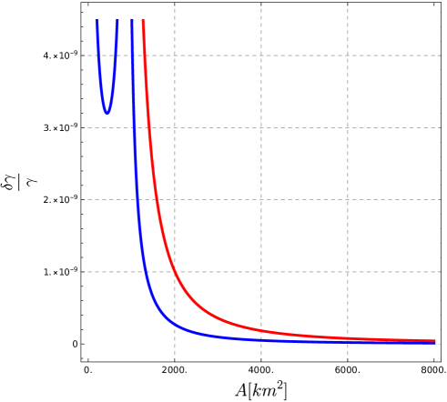
(a)

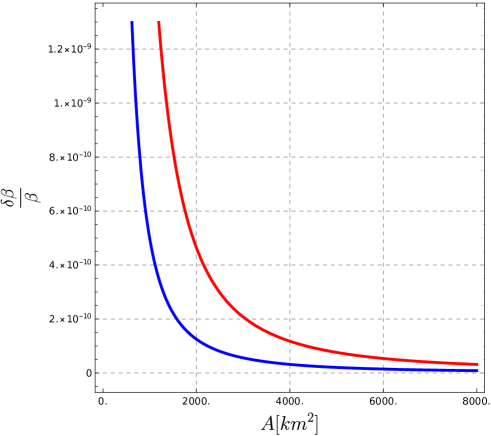
(b)

Figure 9: Relative error of the parameters $\gamma$ and $\beta$ measured through the probability of detection Eq. (24), in terms of the area $A=\Delta h\times L_{\gamma_{2}}$ of the array. (a) Relative error parameter $\gamma$. (b) Relative error parameter $\beta$. For both simulations the uncertainty in the measure of the probability of detection is $\delta S=10^{-13}$. We assume that in both HOM array configuration the uncertainty in the probability of detection is the same. In the array configuration, given an area $A_{1}$ for the detection of the first time delay, the second area $A_{2}=\eta A_{1}$, where $\eta=1/4$. Blue continuous line represents the squeezing parameter $r=1$, red continuous line $r=2$. The mean wavelength of both photons is $\lambda=0.995\;[\mu m]$ and a bandwidth $\delta\lambda=0.034\;[\mu m]$.

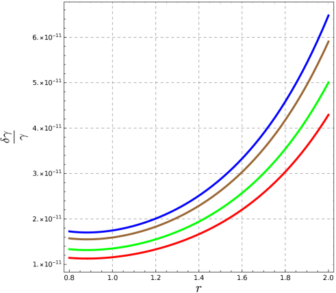
(a)

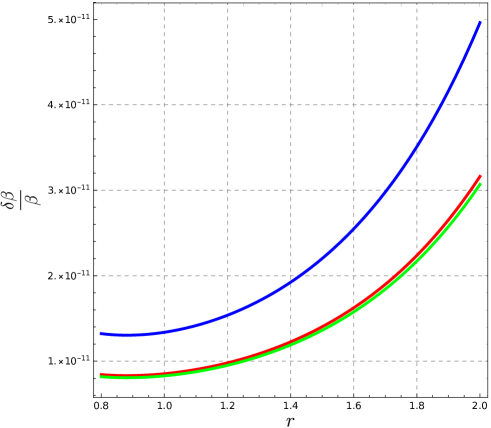
(b)

Figure 10: Relative error of the parameter $\gamma$ and $\beta$ measured through the probability of detection Eq. (24), in terms of the squeezing parameter $r$. (a) Relative error for the parameter $\gamma$. (b) Relative error for the parameter $\beta$. For both simulations the uncertainty in the measure of the probability of detection is $\delta S=10^{-13}$. We assume that, in both HOM array configurations, the uncertainty in the probability of detection is the same. In the array configuration, given an area $A_{1}$ for the detection of the first time delay, the second area $A_{2}=\eta A_{1}$, where $\eta$ is a constant. Continuous blue line $\eta=1/8$, continuous red line $\eta=1/4$, continuous green line $\eta=1/2$. For (a) Continuous brown line $\eta=1$. The mean wavelength of both photons is $\lambda=0.995\;[\mu m]$ and a bandwidth $\delta\lambda=0.034\;[\mu m]$.

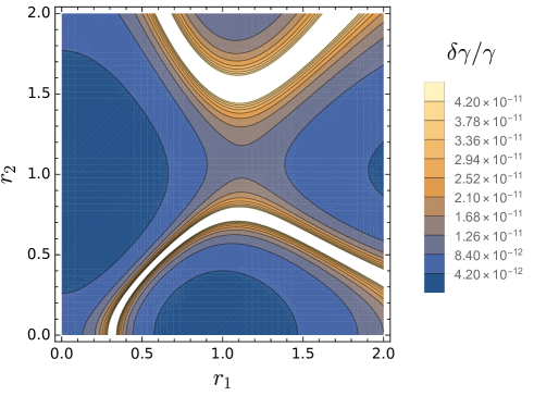
(a)

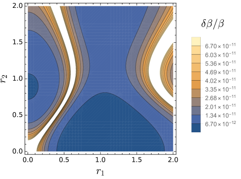
(b)

Figure 11: Contour plot of the relative error of the parameters $\gamma$ and $\beta$ measured through the probability of detection Eq. (24), in terms of the squeezing parameters $r_{1}$ and $r_{2}$, employed in the first and second configuration of the HOM array, respectively. (a) Relative error parameter $\gamma$. (b) Relative error parameter $\beta$. The uncertainty in the measure of the probability of detection is $\delta S=10^{-13}$. We assume that, in both HOM array configurations, the uncertainty in the probability of detection is the same.In the array configuration, $A_{1}$ is the area for the first array configuration, in which the detection of the first time delay is done. The second array has area $A_{2}=\eta A_{1}$, with $\eta=1/4$. The mean wavelength of both photons is $\lambda=0.995\;[\mu m]$ and a bandwidth $\delta\lambda=0.034\;[\mu m]$.

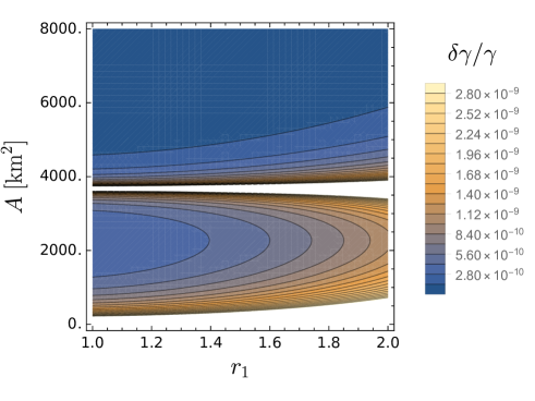
(a)

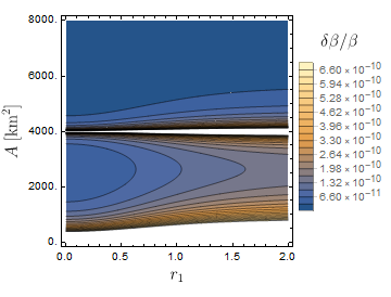
(b)

Figure 12: Contour plot of the relative error of the parameter $\gamma$ measured through the probability of detection Eq. (24), in terms of the squeezing parameters $r_{1}$ ( assumed to be equal in both configurations of the arrays), and the area $A=\Delta h\times L_{\gamma_{2}}$. The uncertainty in the measure of the probability of detection is $\delta S=10^{-13}$. We assume that, in both HOM array configurations, the uncertainty in the probability of detection is the same.In the array configuration, $A_{1}$ is the area for the first array configuration, in which the detection of the first time delay is done. The second array has area $A_{2}=\eta A_{1}$, with $\eta=1/4$. The mean wavelength of both photons is $\lambda=0.995\;[\mu m]$ and a bandwidth $\delta\lambda=0.034\;[\mu m]$.

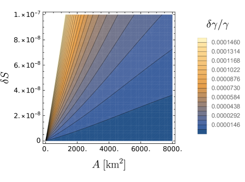
(a)

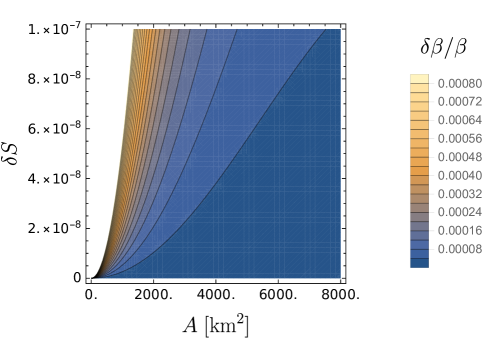
(b)

Figure 13: Contour plot of the relative error of the parameter $\gamma$ and $\beta$ measured through the probability of detection Eq. (24), for a squeezing parameter $r=1$ (assumed to be equal in both configurations of the arrays), in terms of the area $A=\Delta h\times L_{\gamma_{2}}$ and the uncertainty of the measurement of the coincidence operator $\delta S$ Eq. (18). We assume that in both HOM array configurations, the uncertainty in the probability of detection is the same.In the array configuration, $A_{1}$ is the area for the first array configuration, in which the detection of the first time delay is done. The second array has area $A_{2}=\eta A_{1}$, with $\eta=1/4$. The mean wavelength of both photons is $\lambda=0.995\;[\mu m]$ and a bandwidth $\delta\lambda=0.034\;[\mu m]$.

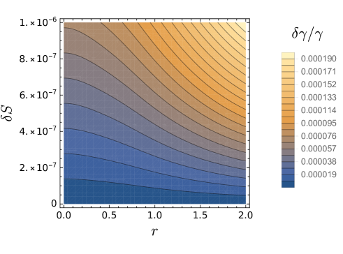
(a)

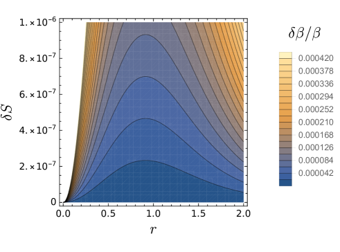
(b)

Figure 14: Contour plot of the relative error of the parameter $\gamma$ and $\beta$ measured through the probability of detection Eq. (24), in terms of the squeezing parameter $r$ and the uncertainty of the measurement of the coincidence operator $S$ Eq. (18). We assume that in both HOM array configurations, the uncertainty in the probability of detection is the same. In the array configuration, $A_{1}$ is the area for the first array configuration, in which the detection of the first time delay is done. The second array has area $A_{2}=\eta A_{1}$, with $\eta=1/4$ and $A_{1}=8\times 10^{3}\,[\rm km^{2}]$.

6 Summary and conclusions

We have studied the problem of estimating values of the parameters $\gamma$ and $\beta$ of the post-Newtonian expansion. For this purpose, we have considered a basic setup consisting of a HOM interferometer whose arms are at different gravitational potentials. We consider the measurement of two different arrival times in order to obtain an estimation of the PN parameters $\gamma$ and $\beta$. Moreover, we study the case in which ones measures the coincident detection probability. We show that the latter method leads to an improvement in relative errors when compared with classical approaches [6]. We consider two-photon separable states and two-mode squeezed-vacuum states to estimate the values of $\gamma$ and $\beta$. Table 1 shows that relative errors obtained for $\gamma$ and $\beta$ are approximately of the same order of magnitude if we consider two-mode squeezed-vacuum states. Moreover, employing this state we obtain a lower uncertainty in the estimation of the PN parameters even with a higher uncertainty in the measurement of the coincidence operator (see table 2). We emphasize that these schemes rely on the use of specific quantum states of light, which impose conditions on the sources employed to generate the quantum states. Fortunately, these sources are already available and are known as ultra-broadband SPDC sources [28].

One of the advantages of the protocol discussed here is its versatility in terms of the initial states that enter the interferometer. To improve the detection and sensitivity we can employ NOON states or cat states, among many others. An obvious modification of this scheme could be the use of a Mach-Zehnder interferometer and measuring a different observable, instead the coincidence detection observable, as for example the relative number of photons arriving to the output ports [29]. A more realistic implementation should consider loss in the detection [30] or the probability of no detection in the HOM array [13, 9], and include the relative velocity of the satellites [31, 19].

Method	$\delta\gamma/\gamma$	$\delta\beta/\beta$	$\delta S$
Classical tests	$\sim 10^{-5}$	$\sim 10^{-5}$	experiment dependent
Measurement of $\Delta\tau_{i}$ ($i=1,2$)	$\sim 10^{-2}$	$\sim 10^{-11}$	$\sim 10^{-18}$
Separable bipartite state	$\sim 10^{-16}$	$\sim 10^{-7}$	$\sim 10^{-18}$
Two-mode squeezing (r=1)	$\sim 10^{-10}$	$\sim 10^{-11}$	$\sim 10^{-13}$

Table 1: Relative errors for $\gamma$ and $\beta$ given an area of the first array $A_{\rm max}=8\times 10^{3}[km^{2}]$

Method	$\delta S$ for $\gamma$	$\delta S$ for $\beta$
Measurement $\Delta\tau_{i}$ ($i=1,2$)	$\sim 10^{-20}$	$\sim 10^{-15}$
separable biparite state	$\sim 10^{-10}$	$\sim 10^{-16}$
two-mode squeezing ($r=1$)	$\sim 10^{-8}$	$\sim 10^{-8}$

Table 2: Uncertainty necessary to achieve the current uncertainties of $\gamma$ and $\beta$

Appendix A Two mode vacuum states

A two mode vacuum state is given by the Eq. (22). The output state is given by

$$|\zeta_{\rm out}\rangle = \frac{1}{\cosh(r)}\iint d\omega_{1}\omega_{2}f(\omega_{1},\omega_{2})\sum_{n=0}^{\infty}(-1)^{n}e^{in\theta}\left(\tanh(r)\right)^{n}\left[\frac{c^{\dagger}_{\omega_{1}}}{\sqrt{2}}+\frac{d^{\dagger}_{\omega_{1}}}{\sqrt{2}}\right]^{n}e^{-i\omega_{1}\Delta\tau_{\gamma_{1}}}$$

$$\left[\frac{c^{\dagger}_{\omega_{2}}}{\sqrt{2}}-\frac{d^{\dagger}_{\omega_{2}}}{\sqrt{2}}\right]^{n}e^{-i\omega_{2}\Delta\tau_{\gamma_{2}}}|0\rangle_{12},$$

where $\Delta\tau_{\gamma_{1}}$ and $\Delta\tau_{\gamma_{2}}$, are the time delay for the paths $\gamma_{1}$ and $\gamma_{2}$, respectively. In order to simplify the probability of detection we consider $n=1$ squeezing states, under this consideration the probability to detect one photon is given by

$$P_{\rm cd} = \langle\zeta_{\rm out}|\hat{M}_{c}\otimes\hat{M}_{d}|\zeta_{\rm out}\rangle,$$ (52)

where $\hat{M}_{c}=\int d\omega c^{\dagger}_{\omega}|0\rangle\langle 0|c_{\omega}$ and $\hat{M}_{d}=\int d\omega^{\prime}d^{\dagger}_{\omega^{\prime}}|0\rangle\langle 0|d_{\omega^{\prime}}$. The amplitude of probability for $n=1$ reads

$$\langle 1|\langle 1|\zeta_{\rm out}\rangle = \frac{1}{\cosh(r)}\iint d\omega_{1}d\omega_{2}f(\omega_{1},\omega_{2})^{\ast}$$

$$\langle 0|c_{\omega}d_{\omega^{\prime}}\left[e^{-i\omega_{1}\Delta\tau_{\gamma_{1}}}e^{-i\omega_{1}\Delta\tau_{\gamma_{2}}}|0\rangle|0\rangle-e^{i\theta}\frac{\tanh(r)}{2}\left(c^{\dagger}_{\omega_{1}}+d^{\dagger}_{\omega_{1}}\right)\ \left(c^{\dagger}_{\omega_{2}}-d^{\dagger}_{\omega_{2}}\right)|0\rangle\right]$$

$$= -\iint d\omega_{1}d\omega_{2}f(\omega_{1},\omega_{2})^{\ast}\frac{e^{i\theta}\tanh(r)}{2\cosh(r)}\langle 0|c_{\omega}d_{\omega^{\prime}}\left(c^{\dagger}_{\omega_{1}}+d^{\dagger}_{\omega_{1}}\right)\left(c^{\dagger}_{\omega_{2}}-d^{\dagger}_{\omega_{2}}\right)|0\rangle.$$

The non-vanishing terms in the operator are the following

$$\langle 0|-c_{\omega}c^{\dagger}_{\omega_{1}}d_{\omega^{\prime}}d^{\dagger}_{\omega^{\prime}}d^{\dagger}_{\omega_{2}}+c_{\omega}c^{\dagger}_{\omega_{2}}d_{\omega^{\prime}}d^{\dagger}_{\omega^{\prime}}d^{\dagger}_{\omega_{1}}|0\rangle = -\delta(\omega-\omega_{1})\delta(\omega^{\prime}-\omega_{2})+\delta(\omega-\omega_{2})\delta(\omega^{\prime}-\omega_{1}).$$

Therefore, the probability of detection, in case of $f(\omega_{1},\omega_{2})=f(\omega_{1})f(\omega_{2})$, with $f(\omega_{i})$ a Gaussian distribution centred in $\omega_{i}$, reads

$$P_{\rm cd} = \frac{1}{2}\left(\frac{\tanh(r)}{\cosh(r)}\right)^{2}\left[1-\exp\left(-\sigma^{2}\Delta\tau^{2}/2\right)\right],$$ (55)

where $\sigma$ is the spectral width of the Gaussian distribution, assumed to be equal for both photons.

References

- [1] Gerard Auger and Eric Plagnol “An Overview of Gravitational Waves” WORLD SCIENTIFIC, 2017 DOI: 10.1142/10082
- [2] Clifford M. Will “On the unreasonable effectiveness of the post-Newtonian approximation in gravitational physics” In Proceedings of the National Academy of Sciences 108.15 National Academy of Sciences, 2011, pp. 5938–5945 DOI: 10.1073/pnas.1103127108
- [3] C.M Will “The Confrontation between General Relativity and Experiment” In Living Rev. Relativ. 17.4, 2014 DOI: 10.12942/lrr-2014-4
- [4] Stephen M. Merkowitz “Tests of Gravity Using Lunar Laser Ranging” In Living Reviews in Relativity 13.7, 2010 DOI: 10.12942/lrr-2010-7
- [5] Magdalena Zych al. “General relativistic effects in quantum interference of photons” In Classical and Quantum Gravity 29.22 IOP Publishing, 2012, pp. 224010 DOI: 10.1088/0264-9381/29/22/224010
- [6] Clifford M. Will “The Confrontation between General Relativity and Experiment” In Living Reviews in Relativity 17.4, 2014 DOI: 10.12942/lrr-2014-4
- [7] Timothy Clifton “Parametrized post-Newtonian limit of fourth-order theories of gravity” In Phys. Rev. D 77 American Physical Society, 2008, pp. 024041 DOI: 10.1103/PhysRevD.77.024041
- [8] C. K. Hong, Z. Y. Ou and L. Mandel “Measurement of subpicosecond time intervals between two photons by interference” In Phys. Rev. Lett. 59 American Physical Society, 1987, pp. 2044–2046 DOI: 10.1103/PhysRevLett.59.2044
- [9] Ashley Lyons et al. “Attosecond-resolution Hong-Ou-Mandel interferometry” In Science Advances 4.5 American Association for the Advancement of Science, 2018 DOI: 10.1126/sciadv.aap9416
- [10] Jian-Wei Pan et al. “Multiphoton entanglement and interferometry” In Rev. Mod. Phys. 84 American Physical Society, 2012, pp. 777–838 DOI: 10.1103/RevModPhys.84.777
- [11] Yingwen Zhang et al. “Engineering two-photon high-dimensional states through quantum interference” In Science Advances 2.2 American Association for the Advancement of Science, 2016 DOI: 10.1126/sciadv.1501165
- [12] B. Ndagano and A. Forbes “Entanglement distillation by Hong-Ou-Mandel interference with orbital angular momentum states” In APL Photonics 4.1, 2019, pp. 016103 DOI: 10.1063/1.5079970
- [13] Y. Chen, M. Fink and F. et al. Steinlechner In npj Quantum Information 5, 2019 DOI: 10.1038/s41534-019-0161-z
- [14] I. Fuentes-Schuller and R. B. Mann “Alice Falls into a Black Hole: Entanglement in Noninertial Frames” In Phys. Rev. Lett. 95 American Physical Society, 2005, pp. 120404 DOI: 10.1103/PhysRevLett.95.120404
- [15] Miguel Montero and Eduardo Martín-Martínez “Entanglement of arbitrary spin fields in noninertial frames” In Physical Review A 84.1 American Physical Society (APS), 2011 DOI: 10.1103/physreva.84.012337
- [16] Matthias Fink et al. “Experimental test of photonic entanglement in accelerated reference frames” In Nature Communications 8.1 Springer ScienceBusiness Media LLC, 2017 DOI: 10.1038/ncomms15304
- [17] Aharon Brodutch et al. “Post-Newtonian gravitational effects in optical interferometry” In Phys. Rev. D 91 American Physical Society, 2015, pp. 064041 DOI: 10.1103/PhysRevD.91.064041
- [18] Anthony Brady and Stav Haldar “Relativistic frame-dragging and the Hong-Ou-Mandel dip a primitive to gravitational effects in multi-photon quantum-interference”, 2020
- [19] Daniel R. Terno, Giuseppe Vallone, Francesco Vedovato and Paolo Villoresi “Large-scale optical interferometry in general spacetimes” In Phys. Rev. D 101 American Physical Society, 2020, pp. 104052 DOI: 10.1103/PhysRevD.101.104052
- [20] S. Y. Chen and T. C. Ralph “Estimation of gravitational acceleration with quantum optical interferometers” In Phys. Rev. A 99 American Physical Society, 2019, pp. 023803 DOI: 10.1103/PhysRevA.99.023803
- [21] A Delgado, W P Schleich and G Süssmann “Quantum gyroscopes and Gödel's universe: entanglement opens a new testing ground for cosmology” In New Journal of Physics 4 IOP Publishing, 2002, pp. 37–37 DOI: 10.1088/1367-2630/4/1/337
- [22] Endre Kajari, Reinhold Walser, Wolfgang P. Schleich and Aldo Delgado “Sagnac Effect in Gödel’s Universe” In Frontiers in Optics Optical Society of America, 2006, pp. JWD48 DOI: 10.1364/FIO.2006.JWD48
- [23] M Rivera-Tapia, A Delgado and G Rubilar “Weak gravitational field effects on large-scale optical interferometric Bell tests” In Classical and Quantum Gravity 37.19 IOP Publishing, 2020, pp. 195001 DOI: 10.1088/1361-6382/ab8a60
- [24] Jan Kohlrus, David Edward Bruschi and Ivette Fuentes “Quantum-metrology estimation of spacetime parameters of the Earth outperforming classical precision” In Phys. Rev. A 99 American Physical Society, 2019, pp. 032350 DOI: 10.1103/PhysRevA.99.032350
- [25] S. P. Kish and T. C. Ralph “Quantum metrology in the Kerr metric” In Phys. Rev. D 99 American Physical Society, 2019, pp. 124015 DOI: 10.1103/PhysRevD.99.124015
- [26] Graham M Shore “Quantum gravitational optics” In Contemporary Physics 44.6 Taylor & Francis, 2003, pp. 503–521 DOI: 10.1080/00107510310001617106
- [27] Clifford M Will “Theory and experiment in gravitational physics” Cambridge university press, 2018
- [28] Aron Vanselow, Paul Kaufmann, Helen M. Chrzanowski and Sven Ramelow “Ultra-broadband SPDC for spectrally far separated photon pairs” In Opt. Lett. 44.19 OSA, 2019, pp. 4638–4641 DOI: 10.1364/OL.44.004638
- [29] Luca Pezzé and Augusto Smerzi “Mach-Zehnder Interferometry at the Heisenberg Limit with Coherent and Squeezed-Vacuum Light” In Physical Review Letters 100.7 American Physical Society (APS), 2008 DOI: 10.1103/physrevlett.100.073601
- [30] S. P. Kish and T. C. Ralph “Estimating spacetime parameters with a quantum probe in a lossy environment” In Phys. Rev. D 93 American Physical Society, 2016, pp. 105013 DOI: 10.1103/PhysRevD.93.105013
- [31] David Rideout al. “Fundamental quantum optics experiments conceivable with satellites—reaching relativistic distances and velocities” In Classical and Quantum Gravity 29.22 IOP Publishing, 2012, pp. 224011 DOI: 10.1088/0264-9381/29/22/224011