Exact densities of loops in O(1) dense loop model and of clusters in critical percolation on a cylinder.

Abstract

We obtain exact densities of contractible and non-contractible loops in the O(1) model on a strip of the square lattice rolled into an infinite cylinder of finite even circumference $L$. They are also equal to the densities of critical percolation clusters on forty five degree rotated square lattice rolled into a cylinder, which do not or do wrap around the cylinder respectively. The results are presented as explicit rational functions of $L$ taking rational values for any even $L$. Their asymptotic expansions in the large $L$ limit have irrational coefficients reproducing the earlier results in the leading orders. The solution is based on a mapping to the six-vertex model and the use of technique of Baxter’s T-Q equation.

Keywords: O(n) loop models, percolation, six-vertex model, Baxter’s T-Q equation

1 Introduction

The subject of this Letter, $O(1)$ dense loop model (DLM), is a particular case of $O(n)$ loop models, a class of lattice models of statistical physics formulated in terms of ensembles of paths on the lattices. Having connections with many other models they sometimes provide an alternative convenient language for the analysis. An idea of representing the partition function of the Ising model as a sum over sets of weighted contours comes back to Peierls [1]. The summation over contours with weight $n$ assigned to loops appeared from the polygonal representation of the partition function of the random cluster model [2, 3], which, in turn, is related to the $Q$-state Potts model with $\sqrt{Q}=n.$ Also, a connection of the $O(n)$ loop model with the $O(n)$ vector model, from which the former inherited the $O(n)$ name, suggests that the former can be used to predict the critical behavior of the the latter [4]. The language of $O(n)$ loop models turned out especially efficient within the framework of Coulomb gas and conformal field theory (CFT) [5, 6], while their scaling limit fits naturally into the Schramm-Loewner evolution picture [7].

Here we consider the $O(1)$ DLM formulated as a measure on paths on the two-dimensional square lattice. A path passes through every bond exactly once, and two paths meet at every site without crossing each other, see fig. 1. All path configurations have equal weights.

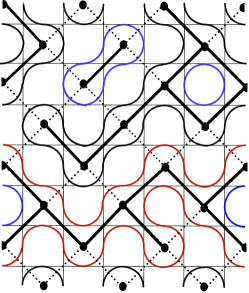
Figure 1: A configuration of the O(1) loop model on the lattice (thin solid lines) and the associated percolation clusters (thick solid lines) on the rotated lattice (dashed lines and black dots). The contractible and non-contractible loops are shown in blue and red respectively.

To construct configurations by local operations we place a vertex at every lattice site, in which two pairs of paths at four incident bonds are connected pairwise in one of two possible ways shown in fig. 2. Both vertices are assigned the unit weight.

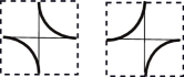
Figure 2: Two vertices of the O(1) loop models. Both vertices have unit weight.

The lattice we consider here is bounded in one spacial direction and unbounded in the other. Specifically, it is a strip of the square lattice, infinite in the direction that coincides with one of the lattice directions, referred to as vertical, and finite in the other (horizontal) direction with even number $L=2N$ of sites. Periodic boundary conditions are implied in the horizontal direction, i.e. the strip is rolled into a cylinder. Under the uniform measure on paths only finite closed loops present on such a cylinder with probability one, each loop having the weight $n=1$.

This model has been intensively studied on its own and especially in view of its connection with the critical bond percolation problem, which is a particular instance of the random cluster model related to a formal $Q\to 1$ limit of the Potts model. To go from loops to percolation we construct a new square lattice of 45 degrees rotated orientation, for which the original lattice is the so called medial graph. To this end, we put sites of the new lattice to the center of every second face of the original lattice in a staggered way, connecting them by bonds passing through the nearest sites of the original lattice as shown in fig. 1. The periodic boundary conditions for the original lattice suggest that the rotated lattice is also rolled into the cylinder. Then, we consider the bond percolation on the lattice constructed. Specifically a bond of the rotated lattice is said to be open, if it is between the loop arcs and closed if it crosses them, see fig. 3. All the four vertices have equal weights, i.e. open and closed bonds have equal probabilities $p=1/2$, which is the critical point of the bond percolation on the infinite square lattice.

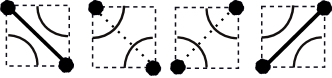
Figure 3: Correspondence between the vertices of O(1) DLM and open (solid) or closed (dashed) bonds on the rotated lattice. The black dots are sites of the rotated lattice.

The studies of percolation having been continuously conducted since the late fifties of the last century culminated in plenty brilliant results, see [8, 9] and references therein. In particular, the connection of percolation with $O(1)$ DLM, in turn related to the exactly solvable six-vertex model, was found especially useful for calculating some observables and critical exponents [10]. In the context of this Letter we mention the calculation of the density of critical percolation clusters on the infinite plane lattice, i.e. in the $L\to\infty$ limit of our cylinder, performed in a seminal paper [11]. The result was obtained in the form of an integral, of which the approximate numerical value was provided. The exact value of the integral was later presented in [12] together with numerical evidences of universality of finite size corrections to this quantity occurring in confined geometries. An explicit form of the finite size corrections to the density of critical percolation clusters on the strip and on the cylinder were conjectured in [13] using arguments based on the Coulomb gas technique and CFT. Specifically, the corrections come from the conformal anomaly, the value of which was found from the mapping of the $O(1)$ DLM to the Coulomb gas [5].

In the $O(1)$ DLM language the quantity related to the density of percolation clusters is the density of loops. In fact, the latter can be considered as a combination of two quantities, which can be studied separately. Indeed, there are two types of loops on the cylinder, contractible and non-contractible, which do not and do wind around the cylinder respectively. Hence, we will be interested in the average numbers of loops of both types per site of the lattice. We will use the notations $\nu_{c}(L)$ and $\nu_{nc}(L)$ for the densities of contractible and non-contractible loops respectively.

To explain the relation of loop densities to the densities of percolation clusters, we note that every contractible loop is either circumscribed on a percolation cluster that does not wrap around the cylinder or is inscribed into a circuit inside a percolation cluster. The latter loop can also be thought as circumscribed on the dual percolation cluster on the dual rotated lattice. The critical point is self-dual. This means that the average numbers of percolation clusters and of dual percolation clusters are equal, and so are the average numbers of the circumscribed and the inscribed loops. Thus, the average number of non-contractible loops per unit length of the cylinder is twice the average number of the critical percolation clusters on the rotated lattice. Since the rotated lattice contains twice less sites per unit length of the cylinder than the original lattice, the density of percolation clusters not wrapping around the cylinder coincides with $\nu_{c}(L)$.

Also every percolation cluster that wraps around the cylinder is bounded by a pair of non-contractible loops and every non-contractible loop runs along the boundary of such a cluster. Thus, similarly to the above, we argue that $\nu_{nc}(L)$ coincides with the average number of critical percolation clusters wrapping around the cylinder per site of the rotated lattice.

How the mean density of non-contractible loops in $O(n)$ model on a cylinder depends on loop weights was studied in [14]. There, the conformal anomaly being a function of the weights of contractible and non-contractible loops was obtained from the finite size correction to the energy of the XXZ chain with twisted boundary conditions [15, 16, 17] divided by a coefficient termed the sound velocity [18]. This allowed a determination of the finite size corrections to the loop densities.

Unfortunately the CFT related arguments applied to models in confined geometries were suitable only for obtaining at most sub-leading terms of the asymptotics of the mean cluster size, while the exact formulas still remained off the scope of this approach. The possibility of the next step opened in the beginning of 2000s. Then, a burst of interest to the $O(1)$ DLM was ignited by an observation by Razumov and Stroganov of a nice combinatorial structure of the ground state of the XXZ chain and the six-vertex model at a specific combinatorial point [19]. A connection of the results of [19] to the $O(1)$ DLM was pointed at in [20]. A number of relations between $O(1)$ DLM, the six vertex model, the XXZ model, the fully packed loop model and alternating sign matrices came from the studies of this subject [21, 22, 23]. In particular, several sum rules for the components of the ground state eigenvector of the $O(1)$ DLM transfer matrix and its generalizations were obtained [24, 25, 26, 27, 28, 29, 30]. Also statistics of several observables describing connectivity of boundary points [31, 32, 33] and loop embeddings [34] on finite lattices were studied in lattices with different boundary conditions like cylinder, strip, e.t.c. For many of them exact formulas were either conjectured or proved. However, to our knowledge, the simplest quantities like the mentioned densities of loops aka the densities of critical percolation clusters are not yet in this list.

In this Letter we fill this gap. We obtain the exact formulas for $\nu_{c}(L)$ and $\nu_{nc}(L)$ for any even $L$. To this end we exploit the connection between the free energies of the $O(n)$ DLM and the six-vertex model. The latter can be found as the largest eigenvalue of the corresponding transfer-matrix, of which the derivatives with respect to the fugacities of contractible and non-contractible loops yield the mean values of interest. The eigenvalue satisfies the Baxter’s T-Q equation as well as the conjugated T-P equation, which are the functional relations between the eigenvalue and two polynomials $Q(x)$ and $P(x)$ having zeroes on the roots of two systems of Bethe equations. Both equations were solved for $Q(x)$ and $P(x)$ in the so called stochastic point, corresponding to the $O(1)$ DLM, by Fridkin, Stroganov, Zagier (FSZ) in [35]. Furthermore, simultaneous differentiation of the transfer-matrix eigenvalue expressed in terms of $Q(x)$ and $P(x)$ and of the Wronskian relation between them allows one to exclude unknown terms and to express the derivatives of the eigenvalue at the stochastic point via the derivatives of the known $Q(x)$ and $P(x)$ in their arguments [36]. The rest of the work and the main technical challenge of this Letter is a reduction of the complicated expressions obtained in terms of the hypergeometric functions evaluated at special values of the parameters and of the argument to a manageable rational form. It is performed with the use of Kummer’s theorem for hypergeometric function and its contiguous generalizations. This is the program we complete in the next sections. Similar calculations were done also in [37] with the eigenvalue of the XXZ chain and in [38] in context of the Raise and Peel model [39].

2 Results

In this section we present the formulas obtained and compare them with the results mentioned above. Stating the results, to avoid an alternate use of the parameters $N$ and $L$, we always use the parameter $N$ implying that $L=2N$.

2.1 Contractible loops

The density of contractible loops is obtained in the form.

$$\nu_{c}(2N) = \frac{3\Gamma\left(\frac{N}{2}\right)\Gamma\left(\frac{3N}{2}+\frac{1}{2}\right)}{4\Gamma\left(\frac{3N}{2}\right)\Gamma\left(\frac{N+1}{2}\right)}+\frac{\pi^{2}2^{-2N}3^{2-3N}\Gamma(3N)}{\Gamma\left(\frac{N}{2}+\frac{1}{6}\right)^{2}\Gamma\left(\frac{N}{2}+\frac{5}{6}\right)^{2}\Gamma(N)}-\frac{5}{2}$$

$$= \frac{1}{8},\frac{17}{160},\frac{913}{8960},\frac{3953}{39424},\frac{14569}{146432},\frac{3945737}{39829504},\dots$$

In the second line we show the numerical values of the quantity obtained for $N=1,\dots,6$. One can see that the densities are rational numbers. Indeed, using the reflection formula for gamma functions the l.h.s of (2.1) can be recast in the form of an explicit rational function of $N$

$$\nu_{c}(2N)=\frac{2^{-2(N+1)}3^{2-3N}\left(2-(-1)^{N}\right)(3N-1)!}{(N-1)!\left(\frac{5}{6}-\frac{N}{2}\right)_{N}^{2}}+\frac{3\left(\frac{N+1}{2}\right)_{N}}{4\left(\frac{N}{2}\right)_{N}}-\frac{5}{2},$$

written in terms of the factorials and the Pochhammer symbols $(a)_{n}=a(a+1)\dots(a+n-1)$. Having no oscillatory factors the formula (2.1) is more suitable for the asymptotical analysis. Using the Stirling formula we obtain an asymptotic expansion, which in the first three orders is

$$\nu_{c}(2N)=\frac{3\sqrt{3}-5}{2}+\frac{1}{4\sqrt{3}}\left(2N\right)^{-2}-\frac{23}{48\sqrt{3}}(2N)^{-4}+O\left(N^{-6}\right).$$ (2)

2.2 Non-contractible loops

The density of non-contractible loops we obtained is

$$\nu_{nc}(2N) =\frac{2^{2(N-2)}\Gamma(N)}{N\pi^{2}\Gamma(3N)} \left(3^{3N}\Gamma\left(\frac{N}{2}+\frac{1}{6}\right)^{2}\Gamma\left(\frac{N}{2}+\frac{5}{6}\right)^{2}-\frac{12\pi^{2}\Gamma\left(\frac{3N}{2}\right)^{2}}{\Gamma\left(\frac{N}{2}\right)^{2}}\right)$$

$$=\frac{1}{8},\frac{11}{320},\frac{421}{26880},\frac{1403}{157696},\frac{4189}{732160},\frac{952067}{238977024},\dots$$

where we again show the first six rational values. The explicitly rational expression of $\nu_{nc}(2N)$ is

$$\nu_{nc}(2N)=\frac{3\times 2^{2(N-1)}(N-1)!}{N(3N-1)!}\left(3^{3N-2}\left(2+(-1)^{N}\right)\left(\frac{5}{6}-\frac{N}{2}\right)_{N}^{2}-\left(\frac{N}{2}\right)_{N}^{2}\right).$$

The Stirling formula applied to (2.2) to three leading orders yields

$$\nu_{nc}(2N)=\frac{1}{\sqrt{3}}(2N)^{-2}-\frac{17}{18\sqrt{3}}\left(2N\right)^{-4}+\frac{1021}{216\sqrt{3}}\left(2N\right)^{-6}+O\left(N^{-8}\right).$$ (4)

2.3 Comparison to earlier results

As one could expect, the leading order term in the asymptotic expansion (2) coincides with the asymptotic value of the critical percolation cluster density on the infinite plane lattice obtained by Temperley and Lieb [11] and promoted to the exact numerical value in [12]. The finite size correction to this value obtained in [13] referred to all (both contractible and non-contractible) loops. It is to be compared to the sum of the sub-leading term in (2) and the leading term in (2.2). Our result differs by the factor of $2$ from that in [13]. This difference stems from the distinction of the length scales between the original and the rotated lattice. Specifically, the result in [13] followed from the CFT prediction [40, 41] for the form of universal finite size correction to the specific free energy on the cylinder of circumference $L$

$$f_{L}=f_{\infty}-\frac{\pi c}{6}L^{-2},$$

where, when applied to the lattice, the length is supposed to be measured in the lattice spacings. As in our case the lattice spacing of the rotated lattice is $\sqrt{2}$, the length $L$ should be replaced by $\sqrt{2}N$, which explains the discrepancy.

The conformal anomaly term used in [14] to evaluate the density of non-contractible loops in $O(n)$ DLM referred to the original lattice. Indeed, the leading term in (2.2) exactly coincides with the value that follows from the formula in [14] with parameters corresponding to unit fugacities of both contractible and non-contractible loops. The sub-leading term of (2) can also be obtained from [14] by differentiation of the anomaly term with respect to the fugacity of contractible loops.

3 From loops to the six-vertex model

The solution is based on the relation between the $O(1)$ DLM and the asymmetric six-vertex model via the directed loop model introduced as follows [3]. We give an orientation to every loop, which now can be either clockwise of anti-clockwise. To this end, we put an arrow in one of two possible directions to each arc within the vertices in fig. 2. Thus we obtain eight vertices of the directed loop model. To obtain six vertices of the six-vertex model out of them we put arrows on the bonds incident to every site in directions consistent with the directions of the arcs, as shown in fig. 4, ignoring the arc connectivities. Then, two vertices of the six-vertex model will be the sums of pairs of vertices of the directed loop model and the other four will be one-to-one. To be short, a summation over the loop orientations within the directed loop model leads us to the undirected DLM, while the summation over the arc connectivities, with information about the arrow directions kept, yields the six-vertex model.

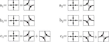
Figure 4: Correspondence between the six-vertex model and the directed loop model.

We assign the following vertex weights using the prescription of [42].

$$a_{1} = ze^{\mathrm{i}\frac{\varphi}{L}},\quad a_{2}=ze^{-\mathrm{i}\frac{\varphi}{L}},$$

$$b_{1} = e^{-\mathrm{i}\frac{\varphi}{L}},\quad b_{2}=e^{\mathrm{i}\frac{\varphi}{L}},$$

$$c_{1} = zq^{1/2}+q^{-1/2},\quad c_{2}=q^{1/2}+zq^{-1/2}.$$

Here $z$ is an auxiliary spectral parameter that will be set equal to one in the end. At $z=1$, the weight choice ensures that the contractible and non-contractible loops come with weights

$$w=2_{q}=q+q^{-1}\quad\mathrm{and\quad v=2cos\varphi,}$$

respectively. In particular we obtain the unit weights, $w=v=1,$ in the so called stochastic point

$$q=e^{\frac{\mathrm{i}\pi}{3}},\quad\varphi=\pi/3,$$ (5)

while the quantities of interest are given by derivatives

$$\nu_{c} = \left.w\frac{d}{dw}\right|_{w=1}f_{L}(w,1),\quad\nu_{nc}=\left.v\frac{d}{dv}\right|_{v=1}f_{L}(1,v)$$ (6)

of the specific free energy $f_{L}(w,v)$. The latter is equal to the logarithm of the largest eigenvalue $\Lambda(z)$ of corresponding row-to-row transfer-matrix normalized to the number of sites $L$ in a horizontal row

$$f_{L}(w,v)=L^{-1}\ln\Lambda_{\max}(1).$$

For the solution of the six vertex model we refer the reader to [43, 44, 10]. To summarize, the transfer matrix describing the transition between two subsequent horizontal rows of vertical bonds can be written in a basis of configurations with fixed positions of up-arrows. Since the action of the transfer matrix preserves the number of up- and down-arrows, the eigenspace is a direct sum of invariant subspaces indexed by the number $M$ of up arrows in a horizontal row, which can take any integer value within the range $0\leq M\leq L$. For $M$ fixed, we use the Bethe ansatz to diagonalize the transfer matrix and obtain the eigenvalues in the form

$$\Lambda(z)=z^{L}e^{\mathrm{i}\varphi}\prod_{i=1}^{M}\frac{1+(z+2_{q})z_{i}e^{-\frac{2\mathrm{i}\varphi}{L}}}{z-z_{i}e^{-\frac{2\mathrm{i}\varphi}{L}}}+e^{-\mathrm{i}\varphi}\prod_{i=1}^{M}\frac{2_{q}z+1+z_{i}ze^{-\frac{2\mathrm{i}\varphi}{L}}}{z_{i}e^{-\frac{2\mathrm{i}\varphi}{L}}-z},$$ (7)

evaluated at numbers $z_{1},\dots,z_{M}$ being the roots of the Bethe ansatz equations (BAE)

$$z_{j}^{L}=\left(-1\right)^{M-1}\prod_{l=1}^{M}\frac{1+e^{-\frac{2\mathrm{i}\varphi}{L}}2_{q}z_{j}+e^{-\frac{4\mathrm{i}\varphi}{L}}z_{l}z_{j}}{1+e^{-\frac{2\mathrm{i}\varphi}{L}}2_{q}z_{l}+e^{-\frac{4i\varphi}{L}}z_{l}z_{j}},\,\,\,i=1,\dots,M.$$ (8)

For further convenience we make a variable change

$$z=\frac{u-q}{1-qu},\quad z_{i}=e^{\frac{2\mathrm{i}\varphi}{L}}\frac{u_{i}-q}{1-qu_{i}},$$

to arrive at the following form of the eigenvalue

$$\Lambda\left(\frac{u-q}{1-uq}\right)=\left(\frac{u-q}{1-uq}\right)^{L}\frac{e^{\mathrm{i}\varphi}}{\left(-q\right)^{M}}\prod_{i=1}^{M}\frac{uq^{2}-u_{i}}{u-u_{i}}+\frac{\left(-q\right)^{M}}{e^{\mathrm{i}\varphi}}\prod_{i=1}^{M}\frac{uq^{-2}-u_{i}}{u-u_{i}}$$ (9)

and the system of BAE for the parameters $u_{1},\dots,u_{M}$ to be substituted to (9)

$$e^{2\mathrm{i}\varphi}\left(\frac{u_{i}-q}{1-qu_{i}}\right)^{L}=\left(-1\right)^{M-1}\prod_{j=1}^{M}\frac{q^{2}u_{j}-u_{i}}{q^{2}u_{i}-u_{j}},\quad i=1,\dots,M.$$ (10)

Every solution of this system yields a particular eigenvalue. A straightforward approach would be to find the solution of (8) corresponding to the largest eigenvalue, to substitute it into (7), and to differentiate. Of course, finding a solution of nonlinear algebraic system explicitly is not a manageable problem. One, however, can get around this problem by writing an equation directly for the eigenvalue. The necessary technique is based on the T-Q equation and its FSZ solution in the stochastic point.

4 T-Q equation and FSZ solution

Alternatively, the eigenvalue problem can be rewritten as a single functional relation for the polynomial

$$Q(u)=\prod_{i=1}^{M}(u-u_{i}),$$

with the roots being a particular solution of (7). To this end we note that the eigenvalue (7) must be polynomial in $z$ of degree at most $L$. Hence the quantity

$$T(u)=\Lambda\left(\frac{u-q}{1-uq}\right)(1-uq)^{L}(-q)^{M-L}$$

is polynomial in $u$ of at most the same degree. In terms of $T(u)$ the formula (9) takes the form

$$T(u)Q(u)=e^{\mathrm{i}\varphi}\phi\left(uq^{-1}\right)Q(uq^{2})+e^{-\mathrm{i}\varphi}\phi\left(uq\right)Q(uq^{-2})(-q)^{2M-L},$$ (11)

where we introduced

$$\phi(u)=\left(1-u\right)^{L}$$ (12)

and multiplied both sides of (9) by the denominator of its r.h.s. A condition of polynomiality of $T(x)$ suggesting that the r.h.s. of (11) is divisible by $Q(u)$, i.e. the Bethe roots are zeroes of r.h.s. of (11), is equivalent to the system (10) of BAE. The idea, however, is to attack the problem by solving the functional relation (11) for two unknown polynomials $T(u)$ and $Q(u)$.

Before going to the solution we introduce a conjugated problem for $T(u)$ and another polynomial $P(u)$ of degree $(L-M).$ This problem arises if we solve the eigenproblem for the transfer-matrix in a different basis keeping track for positions of the down- instead of the up-arrows. This is equivalent to solving the original six-vertex model with the weights $a_{1},b_{1},c_{1}$ and $a_{2},b_{2},c_{2}$ exchanged respectively, which in practice is realized by the change $\varphi\leftrightarrow-\varphi$. Since we did nothing but the change of the basis, the solution of the problem with $(L-M)$ down-arrows should produce the same eigenvalues $\Lambda(z)$. Thus, for $T(u)$ we obtain

$$T(u)P(u)=(-q)^{2M-L}e^{\mathrm{-i}\varphi}\phi\left(uq^{-1}\right)P(uq^{2})+e^{\mathrm{i}\varphi}\phi\left(uq\right)P(uq^{-2}).$$ (13)

Multiplying eqs. (11) and (13) by $P(u)$ and $Q(u)$ respectively, subtracting one from the other and analyzing the structure of zeroes of the terms of equation obtained, we arrive at the quantum Wronskian relation between $Q(u)$and $P(u)$.

$$\phi(u)=\frac{e^{\mathrm{i}\varphi}Q(qu)P(q^{-1}u)-e^{-\mathrm{i}\varphi}Q(q^{-1}u)P(qu)(-q)^{2M-L}}{e^{\mathrm{i}\varphi}(-q)^{2M-L}-e^{-\mathrm{i}\varphi}}$$ (14)

Substituting this into either of (11) or (13) we also obtain

$$T(u)=\frac{e^{\mathrm{2i}\varphi}Q(q^{2}u)P(q^{-2}u)-e^{-2\mathrm{i}\varphi}Q(q^{-2}u)P(q^{2}u)(-q)^{2M-L}}{e^{\mathrm{i}\varphi}(-q)^{2M-L}-e^{-\mathrm{i}\varphi}}.$$ (15)

These two equations are the key formulas for our solution.

Now, we are in a position to proceed with the solution for the largest eigenvalue. This solution corresponds to the choice

$$M=N=L/2.$$ (16)

Thus, the factor $(-q)^{2M-L}$ disappears from the equations (14,15), which then take exactly the form studied in [38]. In this case, the solutions of T-Q and T-P equations for the XXZ chain with anisotropy parameter $\Delta=-1/2$ and twisted boundary conditions corresponding to the stochastic point (5) were found in [36]. Here we keep to the notations of [38] and refer the reader to the formulas in that paper. The solution for $T(x)$ has the form

$$T(x)=(1+x)^{2N}$$ (17)

that in particular suggests $\Lambda(1)=2^{2N}$, which is simply the number of possible arrangements of vertices from fig. 2 within one horizontal row. The polynomials $Q(x)$ and $P(x)$ are looked for in the form

$$Q(x)=f_{Q}(x)(1+x)^{-2N},P(x)=f_{P}(x)\left(1+x\right)^{-2N},$$ (18)

where in our case it is convenient to represent the functions $f_{Q}(x)$ and $f_{P}(x)$ in terms of Gauss hypergeometric function (see [38])

$$f_{Q}(x) = \frac{\Gamma(2/3)}{\Gamma(2/3-N)}\left(\frac{\Gamma(2/3)}{\Gamma(2/3+N)}\left.{}_{2}F_{1}(1/3-N,-N,1/3;-x^{3})\right.\right.$$

$$+ \left.\frac{x^{2}N\Gamma(-2/3)}{\Gamma(1/3+N)}\left.{}_{2}F_{1}(2/3-N,1-N,5/3;-x^{3})\right.\right),$$

$$f_{P}(x) = \frac{\Gamma(2/3+N)}{\Gamma(2/3)}\left(\frac{\Gamma(2/3-N)}{\Gamma(2/3)}\left.{}_{2}F_{1}(2/3-N,-N,2/3;-x^{3})\right.\right.$$

$$+ \left.\frac{xN\Gamma(1/3-N)}{\Gamma(4/3)}\left.{}_{2}F_{1}(1/3-N,1-N,4/3;-x^{3})\right.\right).$$

5 Calculating derivatives.

The final step is to calculate the derivatives (6) of the free energy with respect to fugacities $w$ and $v$ at $v=w=1$. This corresponds to differentiation of the eigenvalue with respect to $q$ and $\varphi$ at the stochastic point. Thus, in terms of $T(u)$ we have

$$\nu_{c} = \frac{1}{2}+\frac{(1-q^{-2})^{-1}}{2N}\frac{d\ln T(1)}{dq},\quad\nu_{nc}=-\frac{1}{2\sqrt{3}N}\frac{d\ln T(1)}{d\varphi},$$ (21)

where the coefficients of the derivatives come from the change of variables $v$ and $w$ in (6) to $q$ and $\varphi$ respectively.

To differentiate $T(1)$ in $q$ we use its expression given by r.h.s. of (15). The result

$$\frac{d\ln T(1)}{dq}=2^{-2N}\left(2A+B\right),$$

consists of two parts. One is from the explicit dependence of r.h.s. of (15) on $q$. The other is from an implicit dependence of $Q(x)$ and $P(x)$ on $q$ via the $q$-dependence of Bethe roots. The first one is encapsulated in the letter $A$. It contains the derivatives with respect to $q$ applied to the arguments of $Q(q^{\pm 2}u)$ and $P(q^{\pm 2}u)$. The coefficient $2$ of $A$ comes from the exponent of $q^{\pm 2}$. The quantity $A$ can explicitly be calculated to

$$\!\!\!\!\!\!\!\!\!\!\!\!\!\!\!\!\!\!\!\!\!\!\!\!\!\!\!\!A=\frac{qQ^{\prime}\left(q^{-2}\right)P\left(q^{2}\right)-Q^{\prime}\left(q^{2}\right)P\left(q^{-2}\right)-q^{-1}Q\left(q^{2}\right)P^{\prime}\left(q^{-2}\right)-q^{-1}Q\left(q^{-2}\right)P^{\prime}\left(q^{2}\right)}{q-q^{-1}}$$

$$\!\!\!\!\!\!\!\!\!\!\!\!\!\!\!\!\!\!\!\!\!\!\!=\frac{1}{\mathrm{i}\sqrt{3}}\Big{\{}qf^{\prime}_{Q}(q^{-2})f_{P}(q^{2})-f^{\prime}_{Q}(q^{2})f_{P}(q^{-2})-q^{-1}f_{Q}(q^{2})f^{\prime}_{P}(q^{-2})-q^{-1}f_{Q}(q^{-2})f^{\prime}_{P}(q^{2})\Big{\}}$$ (22)

$$-2N\Big{\{}(f_{Q}(q^{-2})f_{P}(q^{2})-\frac{1+q^{-1}}{\mathrm{i}\sqrt{3}}f_{Q}(q^{2})f_{P}(q^{-2}))\Big{\}}$$

Here and below we assume that $e^{\mathrm{i}\varphi}=q=e^{\mathrm{i}\pi/3}$ and, hence, $q+q^{-1}=1$, $q-q^{-1}=\mathrm{i}\sqrt{3}$ and $q^{3}=q^{-3}=-1,q^{2}=q^{-4}=-q^{-1}=-q^{5}$, e.t.c. In particular, after differentiating we replace $e^{\pm\mathrm{i}\varphi}$ by $q^{\pm 1}$ respectively. The second part, expressed via the letter $B$, is unknown. However, $B$ can be found from yet another derivative of eq. (14)

$$\left.\frac{d\phi(u)}{dq}\right|_{u=q^{3}}=-A+B=0,$$

which apparently vanishes on one hand and includes $A$ and $B$ on the other. Note that we first differentiate and then substitute $u=q^{3}=-1$. As a result we obtain

$$\frac{d\ln T(1)}{dq} = 3\times 2^{-2N}A.$$ (23)

Similarly for the derivatives in $\varphi$ we have

$$\frac{d\ln T(1)}{d\varphi}=\frac{1}{\sqrt{3}}\left(-1+\frac{2C+D}{2^{2N}}\right),\quad\left.\frac{d\phi(u)}{d\varphi}\right|_{u=q^{3}}=\frac{1}{\sqrt{3}}\left(D-C-2^{2N}\right)=0,$$

with

$$C = q^{2}Q\left(q^{2}\right)P\left(q^{-2}\right)+q^{-2}Q\left(q^{-2}\right)P\left(q^{2}\right)$$

$$= q^{2}f_{Q}(q^{2})f_{P}(q^{-2})+q^{-2}f_{Q}(q^{-2})f_{P}(q^{2}),$$

coming from the explicit dependence on $\varphi$ of the numerators of $T(u)$ and $\phi(u)$ and $D$ being the unknown part. There are also constants not included neither in $C$ nor in $D$, which came from differentiating the denominators. Then we obtain

$$\frac{d\ln T(1)}{d\varphi}=\frac{\sqrt{3}C}{2^{2N}},$$ (25)

which agrees with formula obtained previously in [36] in context of XXZ chain with imaginary magnetic field.

In fact, eqs. (21-25) together with formulas (18-4) already provide explicit answers. However, they are not yet of satisfactory form being sums of hardly computable terms. For example, consider the four quantities $f_{Q}(q^{\pm 2}),f_{P}(q^{\pm 2})$ to be substituted to (22,5). Obtained from (4,4) by setting $x=q^{\pm 2}$ each of them consists of two terms containing the hypergeometric function ${}_{2}F_{1}(a,b,c;t)$ with some parameters $a,b,c$, evaluated at $t=-x^{3}=-1$. Likewise, by direct differentiation of (4,4) with the use of formula

$$\partial\left.{}_{2}F_{1}\right.(a,b,c;t)/\partial t=abc^{-1}\,_{2}F_{1}(a+1,b+1,c+1;t)$$ (26)

the derivatives $f^{\prime}_{Q}(q^{\pm 2})$ and $f^{\prime}_{P}(q^{\pm 2})$ necessary for (22) can be calculated to similar three term expressions. The formulas obtained in this way are not very informative. In particular, they are not suitable for the asymptotic analysis. Our next goal is to transform them to a more tractable form.

To this end, we need to evaluate the hypergeometric functions ${}_{2}F_{1}(a,b,c;-1)$ that appear in $f_{Q}(q^{\pm 2}),f_{P}(q^{\pm 2})$ and in $f^{\prime}_{Q}(q^{\pm 2}),f^{\prime}_{P}(q^{\pm 2})$. The well known Kummer’s theorem [45] gives such an evaluation resulting in a ratio of gamma functions, provided that the relation $c=1+a-b$ between the parameters holds. One can see that the parameters of hypergeometric functions in (4,4) satisfy relations $1+a-b-c=\pm 1$ shifted by $\pm 1$. In addition, according to (26), the derivatives $f^{\prime}_{Q}(q^{\pm 2}),f^{\prime}_{P}(q^{\pm 2})$ in (22) will contain the hypergeometric functions with the argument $t=-1$ and parameters satisfying the original Kummer’s relation as well as the relations $1+a-b-c=\pm 2$ shifted by $\pm 2$. Luckily, contiguous generalizations of the Kummer’s theorem proved in [46] are applicable to these cases. They express the hypergeometric functions at $t=-1$ with parameters satisfying shifted relations as sums of ratios of gamma functions as follows

$$\!\!\!\!\!\!\!\!\!\!\!\!\!\!\!\!\!\!\!\!\!\!\!\!\!\!\!\!\!\!\!\!\!\!{}_{2}F_{1}(a,b,1+a-b+n;-1)=\frac{\Gamma(1+a-b+n)\Gamma(1-b)}{2\Gamma(a)\Gamma(1-b+n)}\sum_{k=0}^{n}(-1)^{k}\left(\begin{array}[]{c}n\\ k\end{array}\right)\frac{\Gamma\left(\frac{a}{2}+\frac{k}{2}\right)}{\Gamma\left(\frac{a}{2}+\frac{k}{2}-b+1\right)},$$ (27)

$$\!\!\!\!\!\!\!\!\!\!\!\!\!\!\!\!\!\!\!\!\!\!\!\!\!\!\!\!\!\!\!\!\!\!{}_{2}F_{1}(a,b,1+a-b-n;-1)=\frac{\Gamma(1+a-b-n)\Gamma(1-b-n)}{2\Gamma(a)\Gamma(1-b-n)}\sum_{k=0}^{n}\left(\begin{array}[]{c}n\\ k\end{array}\right)\frac{\Gamma\left(\frac{a}{2}+\frac{k}{2}\right)}{\Gamma\left(\frac{a}{2}+\frac{k}{2}-b+1-n\right)},$$ (28)

where $n\in\mathbb{N}_{0}$. For example, applying this to (4,4) we obtain

$$\!\!\!\!\!\!\!\!\!\!\!\!\!\!\!\!\!\!\!\!\!\!\!\!\!f_{Q}(q^{\pm 2})=\frac{\pi}{\sqrt{3}}\frac{\Gamma\left(\frac{2}{3}\right)}{\Gamma\left(\frac{2}{3}-N\right)}\Biggl{[}\frac{1}{\Gamma\left(\frac{2}{3}+N\right)\Gamma\left(\frac{1}{3}-N\right)}\left(\frac{\Gamma\left(\frac{1}{6}-\frac{N}{2}\right)}{\Gamma\left(\frac{1}{6}+\frac{N}{2}\right)}+\frac{\Gamma\left(\frac{2}{3}-\frac{N}{2}\right)}{\Gamma\left(\frac{2}{3}+\frac{N}{2}\right)}\right)$$

$$\,\,\,\,\,\,\,\,\,\,\,\,\,\,\,\,\,\,\,\,\,\,\,\,\,\,\,\,\,\,-\frac{q^{\mp 2}}{\Gamma\left(\frac{1}{3}+N\right)\Gamma\left(\frac{2}{3}-N\right)}\left(\frac{\Gamma\left(\frac{1}{3}-\frac{N}{2}\right)}{\Gamma\left(\frac{1}{3}+\frac{N}{2}\right)}+\frac{\Gamma\left(\frac{5}{6}-\frac{N}{2}\right)}{\Gamma\left(\frac{5}{6}+\frac{N}{2}\right)}\right)\Biggr{]}$$

$$\!\!\!\!\!\!\!\!\!\!\!\!\!\!\!\!\!\!\!\!\!\!\!\!f_{P}(q^{\pm 2})=\frac{\Gamma\left(\frac{2}{3}+N\right)}{2\Gamma\left(\frac{2}{3}\right)}\Biggl{[}\left(\frac{\Gamma\left(\frac{1}{3}-\frac{N}{2}\right)}{\Gamma\left(\frac{1}{3}+\frac{N}{2}\right)}+\frac{\Gamma\left(\frac{5}{6}-\frac{N}{2}\right)}{\Gamma\left(\frac{5}{6}+\frac{N}{2}\right)}\right)+q^{\pm 2}\left(\frac{\Gamma\left(\frac{1}{6}-\frac{N}{2}\right)}{\Gamma\left(\frac{1}{6}+\frac{N}{2}\right)}+\frac{\Gamma\left(\frac{2}{3}-\frac{N}{2}\right)}{\Gamma\left(\frac{2}{3}+\frac{N}{2}\right)}\right)\Biggr{]}$$

where we also used the reflection identity

$$\Gamma(z)\Gamma(1-z)=\frac{\pi}{\sin\pi z}$$ (29)

to reduce the number of gamma functions. Similar though longer formulas can also be obtained for $f^{\prime}_{Q}(q^{\pm 2})$ and $f^{\prime}_{P}(q^{\pm 2})$. Substituting the eight obtained expressions into (22,5) we arrive at large sums of rational combinations of gamma functions. The remaining part of the work though tedious is straightforward. It consists in step by step simplification of the obtained expressions with the use of the reflection identity (29), the Legendre duplication formula

$$\Gamma(z)\Gamma(z+1/2)=\sqrt{\pi}2^{1-2z}\Gamma(2z)$$ (30)

and the trigonometric identities. At every step we try to reduce the number of gamma functions and trigonometric functions appearing from the reflection identity. Finally, we arrive at the shortest form we are able to obtain, which being substituted to (23,25) and then to (21) gives us formulas (2.1,2.2).

6 Discussion and outlook

To summarize we have obtained the densities of contractible and non-contractible loops on the square lattice and of critical percolation clusters on the forty-five degree rotated square lattice, both rolled into a cylinder. To this end, we used the mapping of the dense loop model to the six-vertex model, and the method of solution of the T-Q and T-P equations proposed earlier by Fridkin, Stroganov and Zagier. The results must also be related to some correlation functions over the stationary state of the associated Markov chain like it was e.g. in context of its continuous-time analogue Raise and Peel model [38]. Which one, however, is not obvious and requires careful investigation in the more complex discrete framework of the $O(1)$ dense loop model .

It has been shown that the leading orders of the asymptotic expansion reproduce previous results. In particular, the sub-leading order of the density of contractible loops and the leading order of the density of non-contractible loops are known to be universal having a meaning within the conformal field theory. The exact formulas obtained here allow in principle deriving the asymptotic expansion to any finite order. It would be interesting to understand whether the higher order finite size corrections can be combined into quantities with any degree of universality [47].

The used technique must be applicable to a wider class of models. In particular the T-Q equation for the XXZ model with free boundary conditions related to the dense loop model on the strip was solved in [36] and a quantity similar to our (23) was found in terms of $Q$- and $P$-polynomials. No final explicit formulas like those presented here were however obtained. Another direct generalization is to consider the lattice with odd $L$. In this case one infinite path on the cylinder exists and no non-contractible loops present. The technique used here was extended to odd $L$ in [37], where it was applied to the eigenvalue of the Hamiltonian of the XXZ model. No results for the discrete lattice model were yet obtained.

More ambitious problems would be an extension of the technique to obtain exact higher cumulants of loop densities, which were also asymptotically predicted from the conformal field theory arguments in [13]. It would also be of interest to find extensions to loop models related with higher spin [48] or rank [49] integrable systems. Another challenge is the generalization of the technique used here to integrable models at the elliptic level like e.g. eight-vertex model and XYZ spin chain. In principle the parameters analogous to our $q$ and $\varphi$ of the six vertex model can also be introduced in that case [50] as well as the technique of T-Q equation is applicable. This makes potentially possible to evaluate the conjugate ground state observables as the derivatives of the largest eigenvalue with respect to these parameters. Also, there is an analogue of the combinatorial point [51] that shows similarly nice properties and admits obtaining exact analytic results about the ground state eigenvalue [52] and eigenvector [53, 54]. Still it is not known whether an analogue of the FSZ method exists in that case. Also there is no interpretation of the eight-vertex model in terms of loops. Is there an appropriate generalization of the loop picture for that case is an interesting question. The study of these issues in both analytic and combinatorial perspectives is the matter for further investigation.

References

- [1] Peierls R 1936 Proc. Camb. Phil. Soc. 32 477-81
- [2] Fortuin CM, Kasteleyn PW 1972 Physica 57 536-64.
- [3] Baxter RJ, Kelland SB and Wu FY 1976 J. Phys. A: Math. Gen. 9 397-406
- [4] Domany E, Mukamel D, Nienhuis B and Schwimmer A 1981 Nucl. Phys. B 190 279
- [5] Nienhuis B 1987 Coulomb Gas Formulation of Two-dimensional Phase Transitions Phase Transitions and Critical Phenomena vol 11, ed C Domb and J L Lebowitz (New York:Academic) pp 1-51
- [6] Jacobsen J L 2009 Conformal field theory applied to loop models Polygons, polyominoes and polyhedra (LectureNotes in Physics vol 775)ed A J Guttmann (Berlin: Springer) pp 347–424
- [7] Nienhuis B, Kager W 2009 Stochastic Lowner Evolution and the Scaling Limit of Critical Models Polygons, Polyominoes and Polycubes LectureNotes in Physics vol 775 ed A J Guttmann (Berlin: Springer) pp 425-467
- [8] Grimmett G 1999 Percolation (Springer, Berlin, Heidelberg)
- [9] Bollobás B, Riordan O, Percolation 2006 (Cambridge University Press)
- [10] Baxter R J 2016 Exactly solved models in statistical mechanics (Elsevier)
- [11] Temperley H N V and Lieb E 1971 Proc. R. Soc. A 322 251
- [12] Ziff RM, Finch SR, Adamchik VS 1997 Phys. Rev. Lett. 79 3447
- [13] Kleban P, Ziff RM. 1998 Phys. Rev. B 57 R8075.
- [14] Alcaraz FC, Brankov JG, Priezzhev VB, Rittenberg V, Rogozhnikov AM 2014 Phys. Rev. E 90 052138
- [15] Alcaraz F C, Barber M N and Batchelor M T, 1988 Ann. Phys. 182 280-343
- [16] Hamer C J, Quispel G R and Batchelor M T, 1987 J. Phys. A: Math. Gen. 20 5677
- [17] Destri C and De Vega HJ 1989 Phys. Lett. B 223 365
- [18] von Gehlen G and Rittenberg V 1987 J. Phys. A: Math. Gen. 20 227
- [19] Razumov A V and Stroganov Yu G 2001 J. Phys. A: Math. Gen. 34 3185-3190.
- [20] Batchelor M T, de Gier J, Nienhuis B 2001 J. Phys. A: Math. Gen. 34 L265
- [21] Razumov A V and Stroganov Yu G 2004 Theor. Math. Phys. 138 333
- [22] Razumov A V and Stroganov Yu G 2005 Theor. Math. Phys. 142 237
- [23] de Gier J 2005 Discr. Math. 298 365
- [24] Di Francesco P and Zinn-Justin P. 2005 Electron. J. Comb. 12 R6
- [25] Di Francesco P and Zinn-Justin P 2005 J. Phys. A: Math. Gen. 38 L815.
- [26] Zinn-Justin P 2006 Electron. J. Comb. 13 R110
- [27] Di Francesco, P, Zinn-Justin, P. and Zuber, J B 2006 2006 J. Stat. Mech.: Theory Exp. 08 P08011.
- [28] Di Francesco P and Zinn-Justin P 2007 J. Stat. Mech.: Theory Exp. Dec 19;2007(12):P12009.
- [29] Razumov AV, Stroganov YG, Zinn-Justin P. 2007 J. Phys. A: Math. Theor. 40 11827
- [30] Cantini L and Sportiello A 2011 J. Comb. Theor. A 118 1549
- [31] de Gier J, Batchelor M T, Nienhuis B and Mitra S 2002 J. Math. Phys. 43 4135
- [32] Mitra S, Nienhuis B, de Gier J and Batchelor M T 2004 J. Stat. Mech.:: Theory Exp. P09010.
- [33] de Gier J, Jacobsen JL, Ponsaing A2016 SciPost Phys 1 012.
- [34] Mitra S, Nienhuis B. 2004 J. Stat. Mech.: Theory Exp. P10006.
- [35] Fridkin V, Stroganov Y and Zagier D 2000 J. Phys. A: Math. Gen. 33 L121
- [36] Fridkin V, Stroganov Y and Zagier D 2001 J. Stat. Phys. 102 781
- [37] Stroganov YG 2001 Theor. Math. Phys. 129 1596
- [38] Povolotsky AM 2019 J. Stat. Mech.: Theory Exp. 074003
- [39] De Gier J, Nienhuis B, Pearce P A and Rittenberg V 2004 J. Stat. Phys. 114 1
- [40] Blöte HWJ, Cardy JL and Nightingale MP 1986 Phys. Rev. Lett. 56 742
- [41] I. Affleck 1986 Phys. Rev. Lett. 56 746
- [42] Zinn-Justin P 2009 arXiv preprint arXiv:0901.0665.
- [43] E. H. Lieb 1967 Phys. Rev. 162 162
- [44] B. Sutherland 1967 Phys. Rev. Lett. 19 103
- [45] Andrews GE, Askey R, Roy R 1999 Special functions (Cambridge university press)
- [46] Choi J, Rathie AK, and Malani S 2007 Taiwan. J. Math 11 1521-1527
- [47] Privman V, Hohenberg PC, Aharony A 1991 Universal critical-point amplitude relations Phase Transitions and Critical Phenomena ed C Domb and J L Lebowitz vol 14 (Academic, New-York.) p 1.
- [48] Nienhuis B. 1990 Int. J. Mod. Phys. B. 4 929-42.
- [49] Fendley P, Jacobsen JL 2008 J. Phys. A: Math. Theor. 41 215001.
- [50] Bazhanov V V and Mangazeev V V 2007 Nucl. Phys. B 775 225-282
- [51] Razumov A V and Stroganov Y G 2010 Theor. Math. Phys. 164 977-91
- [52] Bazhanov V V and Mangazeev V V 2006 J. Phys. A: Math. Gen. 39 12235–43
- [53] Mangazeev V V and Bazhanov V V 2010 J. Phys. A: Math. Theor. 43 085206
- [54] Zinn-Justin P 2013 Sum rule for the eight-vertex model on its combinatorial line. InSymmetries, integrable systems and representations (Springer, London) pp. 599-637