An Implementation of DF-GHG with Application to Spherical Black Hole Excision

Abstract

We present an implementation of the dual foliation generalized harmonic gauge (DF-GHG) formulation within the pseudospectral code bamps. The formalism promises to give greater freedom in the choice of coordinates that can be used in numerical relativity. As a specific application we focus here on the treatment of black holes in spherical symmetry. Existing approaches to black hole excision in numerical relativity are susceptible to failure if the boundary fails to remain outflow. We present a method, called DF-excision, to avoid this failure. Our approach relies on carefully choosing coordinates in which the coordinate lightspeeds are under strict control. These coordinates are then combined with the DF-GHG formulation. After performing a set of validation tests in a simple setting, we study the accretion of large pulses of scalar field matter on to a spherical black hole. We compare the results of DF-excision with a naive setup. DF-excision proves reliable even when the previous approach fails.

I Introduction

Free-evolution formulations of GR for numerical relativity (NR) are built with a number of requirements in mind. Foremost in this list is that the specific PDE problem to be solved must be well-posed. The easiest way to guarantee well-posedness of the initial value problem is to try and render the equations hyperbolic so that textbook theorems may be applied. This, in turn, requires a choice of gauge. Considering the popular harmonic gauge choice $\Box X^{\underline{\alpha}}=0$ we see already that that such a choice requires a choice of coordinates. But, in case we already have a choice of coordinates in mind that do not satisfy this condition, the latter may be problematic. It turns out that what is really required for hyperbolicity is a sensible choice of tensor basis. If, with this tensor basis fixed we change coordinates it turns out that in many cases the equations remain hyperbolic. This strategy is regularly used within the SpEC numerical relativity code Scheel et al. (2006); SpE to treat compact binary systems with coordinates that are approximately corotating with the system, but always with a single foliation of spacetime by a time coordinate $T$. To overcome this restriction one may turn to the dual-foliation (DF) formalism which, as first presented in Hilditch (2015), allows us to employ a tensor basis associated with coordinates $X^{\underline{\alpha}}=(T,X^{\underline{i}})$ whilst actually working in coordinates $x^{\alpha}=(t,x^{i})$. The DF formalism has been used in a number of places in the literature Hilditch and Ruiz (2018); Hilditch et al. (2018); Schoepe et al. (2018); Hilditch and Schoepe (2019); Gasperin and Hilditch (2019); Duarte and Hilditch (2020); Gasperin et al. (2020); Gautam et al. (2021) for mathematical analysis and is under active investigation for the treatment of future null infinity.

In this paper, we present the first implementation of the dual-foliation generalized harmonic gauge (DF-GHG) formulation of GR, which was made in our pseudospectral code bamps Brügmann (2013); Hilditch et al. (2016). In performing the implementation we have made a number of validation tests, a few of which are presented below. But to try and demonstrate the potential of the formalism, we concentrate primarily on the specific use case of black hole excision. The numerical binary black hole breakthrough Pretorius (2005a); Baker et al. (2006); Campanelli et al. (2006) rests, loosely speaking, on the backs of two different approaches for treating the strong-field region, black hole excision and the moving-puncture method. Each has strengths and weaknesses. Excision, as suggested by Unruh to Thornburg Thornburg (1987) and developed by many authors, see Alcubierre and Brügmann (2001); Seidel and Suen (1992); Anninos et al. (1995); Cook et al. (1998); Thornburg (1999); Shoemaker et al. (2003); Calabrese et al. (2004); Pretorius (2005b); Sperhake et al. (2005) for a selection, relies on the idea that nothing can escape from the black hole region, so it should be possible to simply remove that region from the computational domain without affecting the domain of outer communication whatsoever. This has the advantage that the most violent spacetime region is not treated, and the remaining solution may be reasonably expected to be smooth. There are, however, two important requirements to overcome. First, the intuitive idea that nothing can escape needs to be encoded in a formal sense within the equations. This is not trivial because if the excision boundary flaps around wildly and fails to remain an outflow boundary, then we need to give boundary conditions. Even in the Minkowski spacetime it is possible to introduce an excision boundary that satisfies the first condition, by simply taking a sphere and expanding it radially at the speed of light. Secondly therefore, we must guarantee that the physical domain is not discarded at the speed of light. For this we need to insure that a small part of the black hole region stays within the computational domain. Assuming that the apparent horizon remains inside spatial slices of the event horizon, this could be done by making sure that the apparent horizon remains on the grid. A final, less fundamental, but nevertheless desirable property is to control the coordinate position of the apparent horizon within the domain.

Within the SpEC code these necessary conditions for excision are enforced by choosing spatial coordinates $x^{i}$ with a control system Hemberger et al. (2013) that monitors the position of the apparent horizon and drives the coordinates in a desirable direction. This approach is very effective in practice, but as far as we are aware is not guaranteed never to fail, even in spherical symmetry. It also has the technical disadvantage that because the notion of apparent horizon is quasilocal, it is not obvious that textbook well-posedness results can be applied directly. In this paper we use the DF-GHG formulation with coordinates carefully chosen for excision. Although we work in the spherical setting we believe that it may eventually be possible to use the key ingredients of our method in a more general context, subsuming our coordinate choice within the control system setup. Unsurprisingly the core point of our coordinate choice is the use of an area-locking radial coordinate which, combined with insights from the dynamical horizons framework Hayward (1994); Ashtekar and Krishnan (2003) guarantees the first two properties mentioned above. In the near-future the development presented here also has the important use that it will allow us to generalize our earlier perturbative work Bhattacharyya et al. (2020) on the spherical scalar field within a fixed Schwarzschild background to treat perturbations robustly in the fully nonlinear setting, which the naive approach of Hilditch et al. (2017) was incapable of. These results will be reported upon elsewhere.

We begin in Section II with an overview of the DF-GHG formulation. In Section III we then describe, at the continuum level, each of the coordinate choices that we test in our implementation. In Section IV we give a brief overview overview of the bamps code, before presenting our results in Section V. Finally we conclude in Section VI. Geometric units are used throughout.

II The dual foliation formulation

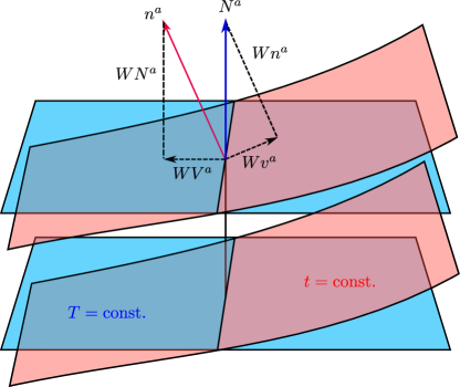
Figure 1: The DF approach: A spacetime with two different slicings and two coordinate systems, the upper case coordinates $(T,X^{\underline{i}})$ and the lower case coordinates $(t,x^{i})$. $N^{a}$ and $n^{a}$ denote the timelike unit normal vectors for the two slices, the inner product of which is the Lorentz factor $W=-(N^{a}n_{a})$. $V^{a}=\frac{1}{W}{}^{\textrm{\tiny{(N)}}}\!\!\!\perp^{b}_{\ a}n_{b}$ and $v^{a}=\frac{1}{W}\perp^{b}_{\ a}N_{b}$ denote the two boost vectors.

In this section, we provide a brief summary of the dual foliation (DF) formalism. Readers interested in a more detailed approach to the topic may look at Hilditch (2015) and Hilditch et al. (2018). The principal idea behind the DF approach is to consider two coordinate systems defined in the same region of spacetime $x^{\mu}=(t,x^{i})$ and $X^{\underline{\mu}}=(T,X^{\underline{i}})$, hereby referred to as the lower case and upper case coordinates respectively. They are shown in Fig. 1. As a matter of convention, Greek indices go over space and time, Latin indices $a,b,c,d,e$ stand for abstract indices, whereas $i,j,k,l,m,p$ represent spatial components in the $x^{\mu}$ basis, and when underlined stand for spatial components in the $X^{\underline{\mu}}$ basis.

The two time coordinates $t$ and $T$ define two foliations of spacetime, the lower case and upper case foliation respectively. In practical applications of the DF formalism we aim to exploit good properties of each coordinate system. As mentioned in the introduction, in our specific setting, this will mean choosing the upper case coordinates (and their associated tensor basis) to be generalized harmonic $\Box X^{\underline{\alpha}}=H^{\underline{\alpha}}$, which is then used to guarantee symmetric hyperbolicity of the field equations we solve. In later sections we will see that we can then choose the lower case coordinates $x^{\mu}$ in a variety of ways, including choices that are useful for black hole excision.

In the lower case foliation, we can define the lapse, normal vector, time vector, projection operator and shift vector as

$$\alpha=(-\nabla_{a}t\nabla^{a}t)^{-\frac{1}{2}}, n^{a}=-\alpha\nabla^{a}t,$$

$$t^{a}\nabla_{a}t\equiv 1, \perp^{a}_{\ b}=\delta^{a}_{\ b}+n^{a}n_{b},$$

$$\beta_{a}=\perp^{b}_{\ a}t_{b}, \beta^{i}=-\alpha n^{a}\nabla_{a}x^{i}.$$ (1)

Similar quantities may be defined in the upper case foliation

$$A=(-\nabla_{a}T\nabla^{a}T)^{-\frac{1}{2}}, N^{a}=-A\nabla^{a}T,$$

$$T^{a}\nabla_{a}T\equiv 1, {}^{\textrm{\tiny{(N)}}}\!\!\!\perp^{a}_{\ b}=\delta^{a}_{\ b}+N^{a}N_{b},$$

$$B_{a}={}^{\textrm{\tiny{(N)}}}\!\!\!\perp^{b}_{\ a}T_{b}, B^{\underline{i}}=-AN^{a}\nabla_{a}X^{\underline{i}}.$$ (2)

The projection operator $\perp^{a}_{\ b}$ with two indices downstairs is the natural induced metric $\gamma_{ab}$ on the lower case foliation and a similar result follows for the upper case foliation where the naturally induced metric is denoted by ${}^{\textrm{\tiny{(N)}}}\gamma_{ab}$. The covariant derivative associated with $\gamma_{ab}$ is denoted by $D$ and the corresponding connection is denoted by $\Gamma$. For the upper case spatial metric ${}^{\textrm{\tiny{(N)}}}\gamma_{ab}$, the associated covariant derivative is ${}^{\textrm{\tiny{(N)}}}D$ and the corresponding connection is ${}^{\textrm{\tiny{(N)}}}\Gamma$.

The relationship between the upper case and the lower case unit normal vector is given by

$$N^{a}=W(n^{a}+v^{a}), n^{a}=W(N^{a}+V^{a}),$$ (3)

where $W$ is called the Lorentz factor and is defined as

$$W=-(N^{a}n_{a})=\frac{1}{\sqrt{1-v_{i}v^{i}}}=\frac{1}{\sqrt{1-V_{\underline{i}}V^{\underline{i}}}},$$ (4)

and $V_{a}$ and $v_{a}$ are the upper case and lower case boost vectors defined as

$$v_{a}=\frac{1}{W}\perp^{b}_{\ a}N_{b}, V_{a}=\frac{1}{W}{}^{\textrm{\tiny{(N)}}}\!\!\!\perp^{b}_{\ a}n_{b}.$$ (5)

The Jacobian matrix, defined as $J^{\underline{\mu}}_{\ \mu}\equiv\partial X^{\underline{\mu}}/\partial x^{\mu}$ can be decomposed in the $3+1$ form

$$n^{\alpha}J^{\underline{\alpha}}_{\ \alpha}N_{\underline{\alpha}}=-W, n^{\alpha}J^{\underline{i}}_{\ \alpha}\equiv\pi^{\underline{i}},$$

$$J^{\underline{\alpha}}_{\ i}N_{\underline{\alpha}}=Wv_{i}, J^{\underline{i}}_{\ i}\equiv\phi^{\underline{i}}_{\ i}.$$ (6)

In matrix form, the Jacobian can be represented as

$$J=\begin{pmatrix}A^{-1}W(\alpha-\beta^{i}v_{i})&\alpha\pi^{\underline{i}}+\beta^{i}\phi^{\underline{i}}_{\ i}\\ -A^{-1}Wv_{i}&\phi^{\underline{i}}_{\ i}\end{pmatrix},$$ (7)

with the inverse being

$$J^{-1}=\begin{pmatrix}\alpha^{-1}W(A-B^{\underline{i}}V_{\underline{i}})&A\Pi^{i}+B^{\underline{i}}\Phi^{i}_{\ \underline{i}}\\ -\alpha^{-1}WV_{\underline{i}}&\Phi^{i}_{\ \underline{i}}\end{pmatrix}.$$ (8)

Note that the quantities $\pi^{\underline{i}}$ and $\Pi^{i}$ can be written in terms of the lapse, shift and boost vectors

$$\pi^{\underline{i}}=WV^{\underline{i}}-WA^{-1}B^{\underline{i}}, \Pi^{i}=Wv^{i}-W\alpha^{-1}\beta^{i}.$$ (9)

Another important result we will need is that for a first order evolution system in upper case coordinates of the form

$$\partial_{T}\bm{u}=(A\bm{A}^{\underline{p}}+B^{\underline{p}}\bm{1})\partial_{\underline{p}}\bm{u}+A\bm{S},$$ (10)

where $\bm{u}$ is the state vector, $\bm{A}^{\underline{p}}$ are the principal matrices, and $\bm{S}$ contains the source terms, can be rewritten in terms of the lower case coordinates as

$$(\bm{1}+\bm{A}^{\underline{V}})\partial_{t}\bm{u} =\alpha W^{-1}\left(\bm{A}^{\underline{p}}(\varphi^{-1})^{p}_{\ \underline{p}}-(\bm{1}+\bm{A}^{\underline{V}})\Pi^{p}\right)\partial_{p}\bm{u}$$

$$\quad+\alpha W^{-1}\bm{S},$$ (11)

where $\varphi^{\underline{i}}_{\ i}={}^{\textrm{\tiny{(N)}}}\gamma^{\underline{i}}_{\ \underline{\mu}}J^{\underline{\mu}}_{\ i}$ is called the projected Jacobian and $\bm{A}^{\underline{V}}\equiv\bm{A}^{\underline{i}}V_{\underline{i}}$.

II.1 DF in the generalized harmonic formulation

In this subsection, we look at the generalized harmonic formalism employed using the dual foliation approach. Our discussion will closely follow Hilditch et al. (2018) but with the addition of the $\gamma_{1}$ parameter, which because of the subtle asymptotics on hyperboloidal slices was earlier hard-coded to vanish. We start essentially with the first order GHG equations of Lindblom et al. (2006) which are in turn based on earlier work of Garfinkle Garfinkle (2002). With the $\gamma_{1}$ parameter turned back on, they read

$$\partial_{T}g_{\underline{\mu\nu}} =(1+\gamma_{1})B^{\underline{i}}\partial_{\underline{i}}g_{\underline{\mu\nu}}+AS^{(g)}_{\underline{\mu\nu}},$$

$$\partial_{T}\Phi_{\underline{i\mu\nu}} =B^{\underline{j}}\partial_{\underline{j}}\Phi_{\underline{i\mu\nu}}-A\partial_{i}\Pi_{\underline{\mu\nu}}+\gamma_{2}A\partial_{\underline{i}}g_{\underline{\mu\nu}}+AS^{(\Phi)}_{\underline{i\mu\nu}},$$

$$\partial_{T}\Pi_{\underline{\mu\nu}} =\gamma_{1}\gamma_{2}B^{\underline{i}}\partial_{\underline{i}}g_{\underline{\mu\nu}}+B^{\underline{i}}\partial_{\underline{i}}\Pi_{\underline{\mu\nu}}-A{}^{\textrm{\tiny{(N)}}}\gamma^{\underline{ij}}\partial_{\underline{i}}\Phi_{\underline{j\mu\nu}}$$

$$\quad+AS^{(\Pi)}_{\underline{\mu\nu}},$$ (12)

where the source terms are given by

$$S^{(g)}_{\underline{\mu\nu}} =-\Pi_{\underline{\mu\nu}}-\gamma_{1}A^{-1}B^{\underline{i}}\Phi_{\underline{i\mu\nu}},$$

$$S^{(\Phi)}_{\underline{i\mu\nu}} =-\gamma_{2}\Phi_{\underline{i\mu\nu}}+\frac{1}{2}N^{\underline{\alpha}}N^{\underline{\beta}}\Phi_{\underline{i\alpha\beta}}\Pi_{\underline{\mu\nu}}+{}^{\textrm{\tiny{(N)}}}\gamma^{\underline{jk}}N^{\underline{\alpha}}\Phi_{\underline{ij\alpha}}\Phi_{\underline{k\mu\nu}},$$

$$S^{(\Pi)}_{\underline{\mu\nu}} =2g^{\underline{\alpha\beta}}\left({}^{\textrm{\tiny{(N)}}}\gamma^{\underline{ij}}\Phi_{\underline{i\alpha\mu}}\Phi_{\underline{j\beta\nu}}-\Pi_{\underline{\alpha\mu}}\Pi_{\underline{\beta\nu}}-g^{\underline{\delta\gamma}}\Gamma_{\underline{\mu\alpha\delta}}\Gamma_{\underline{\nu\beta\gamma}}\right)$$

$$\quad-2\left(\nabla_{(\underline{\mu}}H_{{\underline{\nu}})}+\gamma_{3}\Gamma^{\underline{\alpha}}_{\ \underline{\mu\nu}}C_{\underline{\alpha}}-\frac{1}{2}\gamma_{4}g_{\underline{\mu\nu}}\Gamma^{\underline{\alpha}}C_{\underline{\alpha}}\right)$$

$$\quad-\frac{1}{2}N^{\underline{\alpha}}N^{\underline{\beta}}\Pi_{\underline{\alpha\beta}}\Pi_{\underline{\mu\nu}}-N^{\underline{\alpha}}{}^{\textrm{\tiny{(N)}}}\gamma^{\underline{ij}}\Pi_{\underline{\alpha i}}\Phi_{\underline{j\mu\nu}}$$

$$\quad+\gamma_{0}\left[2\delta^{\underline{\alpha}}_{\ (\underline{\mu}}N_{\underline{\nu})}-g_{\underline{\mu\nu}}N^{\underline{\alpha}}\right]C_{\alpha}-\gamma_{1}\gamma_{2}A^{-1}B^{\underline{i}}\Phi_{\underline{i\mu\nu}},$$ (13)

where we have

$$\Gamma_{\underline{\alpha\mu\nu}} \equiv{}^{\textrm{\tiny{(N)}}}\gamma^{\underline{i}}_{\ (\underline{\mu}|}\Phi_{\underline{i}|\underline{\nu})\underline{\alpha}}-\frac{1}{2}{}^{\textrm{\tiny{(N)}}}\gamma^{\underline{i}}_{\ \underline{\alpha}}\Phi_{\underline{i\mu\nu}}$$

$$\quad+N_{(\underline{\mu}}\Pi_{\underline{\nu})\underline{\alpha}}-\frac{1}{2}N_{\underline{\alpha}}\Pi_{\underline{\mu\nu}},$$ (14)

and the equations are subject to both the reduction constraints

$$C_{\underline{i\mu\nu}}=\partial_{\underline{i}}g_{\underline{\mu\nu}}-\Phi_{\underline{i\mu\nu}},$$ (15)

and the GHG constraints

$$C_{\underline{\mu}}=g^{\underline{\alpha\beta}}\Gamma_{\underline{\mu\alpha\beta}}+H_{\underline{\mu}}=0.$$ (16)

The functions $H_{\underline{\mu}}$ are called the gauge source functions which are functions of the coordinates and the metric. Now, considering these evolution equations to be in the standard form of Eqn. (10), we can easily obtain the $\bm{A}^{\underline{p}}$ matrices which is a slight modification from that given in Hilditch et al. (2018)

$$\bm{A}^{\underline{p}}=\begin{pmatrix}\gamma_{1}A^{-1}B^{\underline{p}}&&0&&0\\ \gamma_{2}\delta^{\underline{p}}_{\ \underline{i}}&&0&&-\delta^{\underline{p}}_{\ \underline{i}}\\ \gamma_{1}\gamma_{2}A^{-1}B^{\underline{p}}&&-{}^{\textrm{\tiny{(N)}}}\gamma^{\underline{pj}}&&0\end{pmatrix}.$$ (17)

To avoid repeating the calculation in Hilditch et al. (2018), we observe that by inclusion of the $\gamma_{1}$ terms within the coordinate change (II) is straightforwardly done by modifying the form given in Hilditch et al. (2018) with the Sherman-Morrison formula. Doing so we arrive at the lower case time evolution equations

$$\partial_{t}g_{\underline{\mu\nu}} =\left(\beta^{p}-\alpha v^{p}+\frac{\gamma_{1}\alpha B^{\underline{p}}}{W(A+B^{V})}(\varphi^{-1})^{p}{}_{\underline{p}}\right)\partial_{p}g_{\underline{\mu\nu}}$$

$$\quad+\alpha W^{-1}s^{(g)}_{\underline{\mu\nu}},$$

$$d_{t}\Phi_{i\underline{\mu\nu}} =\left(\beta^{p}\delta^{j}_{\ i}-\alpha v^{p}\delta^{j}_{\ i}+\alpha W^{2}v_{i}(\mathbbmss{g}^{-1})^{pj}\right)d_{p}\Phi_{j\underline{\mu\nu}}$$

$$\quad+\alpha W^{-1}\mathbbmss{g}^{p}_{\ i}\left(\gamma_{2}\partial_{p}g_{\underline{\mu\nu}}-\partial_{p}\Pi_{\underline{\mu\nu}}\right)+\alpha W^{-1}s^{(\Phi)}_{i\underline{\mu\nu}},$$

$$\partial_{t}\Pi_{\underline{\mu\nu}} =\beta^{p}\partial_{p}\Pi_{\underline{\mu\nu}}-\alpha W(\mathbbmss{g}^{-1})^{pi}d_{p}\Phi_{i\underline{\mu\nu}}+\alpha W^{-1}s^{(\Pi)}_{\underline{\mu\nu}}$$

$$\quad-\gamma_{2}\left(\alpha v^{p}-\frac{\gamma_{1}\alpha B^{\underline{p}}}{W(A+B^{V})}(\varphi^{-1})^{p}{}_{\underline{p}}\right)\partial_{p}g_{\underline{\mu\nu}}.$$ (18)

We use a shorthand notation which abbreviates the contraction with the projected Jacobian

$$d_{\mu}\Phi_{i\underline{\mu\nu}}=\varphi^{\underline{i}}_{\ i}\partial_{\mu}\Phi_{\underline{i\mu\nu}},$$ (19)

and write $B^{V}=B^{\underline{p}}V_{\underline{p}}$. The boost metric is

$$\mathbbmss{g}_{ij}=\gamma_{ij}+W^{2}v_{i}v_{j}.$$ (20)

In terms of the upper case sources, the lower case sources can be written as

$$s^{(g)}_{\underline{\mu\nu}} =\frac{S^{(g)}_{\underline{\mu\nu}}}{1+\gamma_{1}A^{-1}B^{V}},$$

$$s^{(\Phi)}_{\underline{i\mu\nu}} =S^{(\Phi)}_{\underline{i\mu\nu}}+W^{2}V_{\underline{i}}\left(V^{\underline{j}}S^{(\Phi)}_{\underline{j\mu\nu}}-\gamma_{2}S^{(g)}_{\underline{\mu\nu}}+S^{(\Pi)}_{\underline{\mu\nu}}\right),$$

$$s^{(\Pi)}_{\underline{\mu\nu}} =\frac{\gamma_{2}S^{(g)}_{\underline{\mu\nu}}}{1+\gamma_{1}A^{-1}B^{V}}+W^{2}\left(V^{\underline{j}}S^{(\Phi)}_{\underline{j\mu\nu}}-\gamma_{2}S^{(g)}_{\underline{\mu\nu}}+S^{(\Pi)}_{\underline{\mu\nu}}\right).$$ (21)

We take $\mathbbmss{s}_{i}$ to be an arbitrary spatial vector of unit magnitude with respect to it $(\mathbbmss{g}^{-1})^{ij}\mathbbmss{s}_{i}\mathbbmss{s}_{j}=1$ and define a projection operator orthogonal to $\mathbbmss{s}_{i}$ by

$${}^{\mathbbmss{q}}\!\!\!\perp^{i}{\!\!}_{j}=\gamma^{i}{}_{j}-(\mathbbmss{g}^{-1})^{ik}\mathbbmss{s}_{k}\mathbbmss{s}_{j}.$$ (22)

The characteristic variables of the system are given by

$$u^{\hat{0}}_{\underline{\mu\nu}} =g_{\underline{\mu\nu}},$$

$$u^{\hat{B}}_{i\underline{\mu\nu}} ={}^{\mathbbmss{q}}\!\!\!\perp^{j}{\!\!}_{i}\Phi_{j\underline{\mu\nu}}+W\ {}^{\mathbbmss{q}}\!\!\!\perp^{j}{\!\!}_{i}v_{j}(\Pi_{\underline{\mu\nu}}-\gamma_{2}g_{\underline{\mu\nu}}),$$

$$u^{\hat{\pm}}_{\underline{\mu\nu}} =\Pi_{\underline{\mu\nu}}\mp\frac{W}{\sqrt{1+(v^{\mathbbmss{s}})^{2}}}(\mathbbmss{g}^{-1})^{ij}\mathbbmss{s}_{j}\Phi_{i\underline{\mu\nu}}-\gamma_{2}g_{\underline{\mu\nu}},$$ (23)

with the corresponding characteristic speeds

$$\beta^{\mathbbmss{s}}-\alpha\,v^{\mathbbmss{s}}+\gamma_{1}\frac{B^{\underline{p}}(\varphi^{-1})^{p}{}_{\underline{p}}\mathbbmss{s}_{p}}{A+\gamma_{1}B^{V}}\,,$$

$$\beta^{\mathbbmss{s}}-\alpha\,v^{\mathbbmss{s}}\,,$$

$$\beta^{\mathbbmss{s}}\pm\alpha\sqrt{1+(v^{\mathbbmss{s}})^{2}}.$$ (24)

II.2 DF scalar field

For completeness, in this section, we compute the field equations for the scalar field project employing the DF formalism. This calculation is directly analogous to that in the last subsection. We start with the first order form of the scalar field equations written in the upper case coordinates

$$\partial_{T}\Phi =B^{\underline{i}}\partial_{\underline{i}}\Phi+AS^{(\Phi)},$$

$$\partial_{T}\chi_{\underline{i}} =B^{\underline{j}}\partial_{\underline{j}}\chi_{\underline{i}}+A\partial_{\underline{i}}\Pi+\gamma A\partial_{\underline{i}}\Phi+AS^{(\chi)}_{\underline{i}},$$

$$\partial_{T}\Pi =B^{\underline{i}}\partial_{\underline{i}}\Pi+A{}^{\textrm{\tiny{(N)}}}\gamma^{\underline{ij}}\partial_{\underline{j}}\chi_{\underline{i}}+AS^{(\Pi)}.$$ (25)

where the source terms are given by

$$S^{(\Phi)} =\Pi,$$

$$S^{(\chi)}_{\underline{i}} =A^{-1}\chi_{\underline{j}}\partial_{\underline{i}}B^{\underline{j}}+A^{-1}\Pi\partial_{\underline{i}}A-\gamma\chi_{\underline{i}},$$

$$S^{(\Pi)} =K\Pi+A^{-1}\chi_{\underline{i}}{}^{\textrm{\tiny{(N)}}}\gamma^{\underline{ij}}\partial_{\underline{j}}A-{}^{\textrm{\tiny{(N)}}}\gamma^{\underline{ij}}{}^{\textrm{\tiny{(3)}}}\Gamma^{\underline{k}}_{\ \underline{ij}}\chi_{\underline{k}}.$$ (26)

The first order system is of the form given in Eqn. (10), therefore we can construct the principal matrices as

$$\mathbf{A}^{\underline{p}}=\begin{pmatrix}0&0&0\\ \gamma\delta^{\underline{p}}_{\ \underline{i}}&0&\delta^{\underline{p}}_{\ \underline{i}}\\ 0&{}^{\textrm{\tiny{(N)}}}\gamma^{\underline{pj}}&0\end{pmatrix}.$$ (27)

As mentioned in Hilditch et al. (2018), when the Lorentz factor $W$ is bounded, it is possible to invert the coefficient $\left(\mathbf{1}+\mathbf{A}^{\underline{V}}\right)$, which gives

$$\left(\mathbf{1}+\mathbf{A}^{\underline{V}}\right)^{-1}=\begin{pmatrix}1&0&0\\ -\gamma W^{2}V_{\underline{i}}&{}^{\textrm{\tiny{(N)}}}\mathbbmss{g}^{\underline{j}}_{\ \underline{i}}&W^{2}V_{\underline{i}}\\ -\gamma(W^{2}-1)&W^{2}V^{\underline{j}}&W^{2}\end{pmatrix},$$ (28)

where ${}^{\textrm{\tiny{(N)}}}\mathbbmss{g}^{\underline{j}}_{\ \underline{i}}={}^{\textrm{\tiny{(N)}}}\gamma^{\underline{j}}_{\ \underline{i}}+W^{2}V^{\underline{j}}V_{\underline{i}}$. Using this information in Eqn. (II), we arrive at the evolution equation for the scalar field variables in the lower case coordinates

$$\partial_{t}\Phi =\left(\beta^{p}-\alpha v^{p}\right)\partial_{p}\Phi+\alpha W^{-1}s^{(\Phi)},$$

$$d_{t}\chi_{i} =\left(\beta^{p}\delta^{j}_{\ i}-\alpha v^{p}\delta^{j}_{\ i}+\alpha W^{2}v_{i}(\mathbbmss{g}^{-1})^{pj}\right)d_{p}\chi_{j}$$

$$\quad+\alpha W^{-1}\mathbbmss{g}^{p}_{\ i}\left(\gamma\partial_{p}\Phi+\partial_{p}\Pi\right)+\alpha W^{-1}s^{(\chi)}_{i},$$

$$\partial_{t}\Pi =\beta^{p}\partial_{p}\Pi+\gamma\alpha v^{p}\partial_{p}\Phi+\alpha W(\mathbbmss{g}^{-1})^{pi}d_{p}\chi_{i}$$

$$\quad+\alpha W^{-1}s^{(\Pi)}.$$ (29)

Here again we use a shorthand notation which abbreviates contraction with the projected Jacobian

$$d_{\mu}\chi_{i}=\varphi^{\underline{i}}_{\ i}\partial_{\mu}\chi_{\underline{i}}.$$ (30)

In terms of the upper case sources the lower case sources become

$$s^{(\Phi)} =S^{(\Phi)},$$

$$s^{(\chi)}_{\underline{i}} =S^{(\chi)}_{\underline{i}}+W^{2}V_{\underline{i}}\left(V^{\underline{j}}S^{(\chi)}_{\underline{j}}-\gamma S^{(\Phi)}-S^{(\Pi)}\right),$$

$$s^{(\Pi)} =-\gamma S^{(\Phi)}-W^{2}\left(V^{\underline{j}}S^{(\chi)}_{\underline{j}}-\gamma S^{(\Phi)}-S^{(\Pi)}\right).$$ (31)

The characteristic variables of the system are given by

$$u^{\hat{0}} =\Phi,$$

$$u^{\hat{B}}_{j} ={}^{\mathbbmss{q}}\!\!\!\perp^{i}{\!\!}_{j}\;\chi_{i}-W\ {}^{\mathbbmss{q}}\!\!\!\perp^{i}{\!\!}_{j}\,v_{i}\Pi,$$

$$u^{\hat{\pm}} =-\Pi\mp\frac{W}{\sqrt{1+(v^{\mathbbmss{s}})^{2}}}(\mathbbmss{g}^{-1})^{ij}\mathbbmss{s}_{j}\chi_{i}-\gamma\Phi,$$ (32)

with the corresponding characteristic speeds

$$\beta^{\mathbbmss{s}}-\alpha\,v^{\mathbbmss{s}}\,,\quad\beta^{\mathbbmss{s}}-\alpha\,v^{\mathbbmss{s}}\,,\quad\beta^{\mathbbmss{s}}\pm\alpha\sqrt{1+(v^{\mathbbmss{s}})^{2}}.$$ (33)

Here $\mathbbmss{s}$ again denotes an arbitrary unit vector which is normalized against the boost metric and is spatial with respect to $n^{a}$.

III DF Jacobians

In this paper, we are going to present the first numerical tests with DF-GHG with an aim to not only change the spatial coordinates Hemberger et al. (2013) but also the foliation. DF-GHG is implemented in 3d but for now we focus on spherical tests. To demonstrate that everything in the code is correct, we implement a list of Jacobians, some analytic and some that require the evolution of additional fields. As a sanity check, the simplest Jacobian that we implement is the identity Jacobian

$$t=T, x^{i}=X^{\underline{i}},$$ (34)

which of course gives the correct result that we would expect in a run without DF when the same gamma parameters are chosen for the job. Although these Jacobians are primarily built for use in spherically symmetric spacetimes, the implementation itself is made in our fully 3d code. This has the twin advantages that, using the Cartoon method Alcubierre et al. (2001); Pretorius (2005b) for symmetry reduction, we can develop and turn around simulations very quickly, but simultaneously end up with code that can be used in a more general context. In the following subsections we consider:

Analytic Jacobians

In these tests the two sets of coordinates are related by given closed form expressions. The new aspect is that in the past all simulations were performed under the simplifying assumption $T=t$.

Vanishing shift Jacobian

Close to the threshold of black hole formation in vacuum there are indications Hilditch et al. (2017) that popular choices of generalized harmonic coordinates form coordinate singularities. It is known that asymptotically flat spacetimes can always be foliated using a vanishing shift, which this Jacobian choice enforces.

Areal radius Jacobian

In spherical symmetry there is a close relationship between the geometric radial coordinate and the null expansion. In this Jacobian we exploit this relationship to build coordinates in which (as long as we excise close enough to the apparent horizon) the excision boundary remains outflow for sure, and for which the apparent horizon is guaranteed to stay in the computational domain.

DF-excision Jacobian

This Jacobian is an adjustment to the previous setup in which we use a solution to the eikonal equation to get tight control also over the incoming coordinate light speeds.

Alternative choices will be presented in future work.

III.1 Analytic Jacobians

First we consider the analytic Jacobian described by the following relations

$$t=T, x^{i}=f(t,r)X^{\underline{i}}.$$ (35)

Here we choose $f_{1}(t,r)$ such that at $t=0$ and for large radius, the upper case and the lower case coordinates match with each other. We do not yet have provisions for the applying outer boundary conditions in the DF case, so at large radius we require the coordinates to change back to GHG where the usual GHG boundary conditions in bamps can be applied. A choice for $f$ which satisfies these conditions is given by

$$f(t,r)=1+t^{2}A_{1}e^{-(r-r_{0})^{2}}e^{-(t-t_{0})^{2}},$$ (36)

where the Gaussian is centered such that its values approximately reach machine precision or less near the outer boundary. Likewise, we consider another Jacobian which is described by the following relations

$$t=f(t,r)T, x^{i}=X^{\underline{i}}.$$ (37)

III.2 Vanishing shift Jacobian

The vanishing shift Jacobian which keeps the lower case shift zero at all times. Such a choice of coordinates may be useful when performing simulations of gravitational collapse. First we choose

$$t=T,$$ (38)

which makes some other quantities trivial, that is

$$W=1, \alpha=A, V^{\underline{i}}=0, v^{i}=0.$$ (39)

With these choices, we can write down the first of Eqn. (9) as

$$\pi^{\underline{i}}=-A^{-1}B^{\underline{i}}.$$ (40)

This also simplifies the evolution equation for $\phi^{\underline{i}}_{\ i}$ in Eqn. (7) which can be obtained using Cartan’s magic formula Hilditch (2015)

$$\partial_{t}\phi^{\underline{i}}_{\ i}=-D_{i}B^{\underline{i}}+\mathcal{L}_{\beta}\phi^{\underline{i}}_{\ i}.$$ (41)

The first term in the right hand side of the above equation can be considered a source term, because by addition of the reduction constraints, given in Eqn. (15), all first derivatives of metric components can be replaced by evolved variables, whereas the second term should be ideally zero since we want the lower case lapse to be zero. However, since we do not yet have outer boundary conditions in the lower case coordinates, we will employ a transition function approach. In this approach, we choose

$$\beta^{i}=\Omega(r)B^{\underline{i}},$$ (42)

where $\Omega$ is zero at small radii and transitions to one at large radii. This allows us to apply the standard GHG boundary conditions for the outer boundary.

The first source term in Eqn. (41) can be written as

$$\partial_{i}B^{\underline{i}}=J^{\underline{k}}_{\ i}\partial_{\underline{k}}B^{\underline{i}}.$$ (43)

The upper case spatial derivatives of the upper case shift can then be written down in terms of the lapse, shift, extrinsic curvature and the Christoffel symbols, the expressions for which are given below Alcubierre (2008)

$$\partial_{\underline{m}}B^{\underline{l}} =\Gamma^{\underline{l}}_{\ \underline{m0}}+B^{\underline{l}}\Gamma^{\underline{0}}_{\ \underline{m0}}+AK^{\underline{l}}_{\ \underline{m}}$$

$$\quad-B^{\underline{n}}\Gamma^{\underline{l}}_{\ \underline{mn}}-B^{\underline{l}}B^{\underline{n}}\Gamma^{\underline{0}}_{\ \underline{mn}},$$ (44)

where further we use the expressions for the extrinsic curvature

$$K_{\underline{ij}}=-A\Gamma^{\underline{0}}_{\ \underline{ij}}.$$ (45)

The Lie derivative term in Eqn. (41) is only non-vanishing for the subpatch where the transition happens and for all outer subpatches. It can be written down as

$$\mathcal{L}_{\beta}\phi^{\underline{i}}_{\ i}=\Omega B^{\underline{k}}\partial_{k}\phi^{\underline{i}}_{\ i}+\phi^{\underline{i}}_{j}\partial_{i}\beta^{j},$$ (46)

where

$$\partial_{i}\beta^{j}=(\partial_{r}\Omega)\Theta^{\underline{i}}B^{\underline{j}}+\Omega(\partial_{i}B^{\underline{j}}).$$ (47)

where $\Theta^{i}$ are functions of the angular coordinates which are same for both the upper case and lower case coordinates and are related to the Cartesian coordinates by the relation

$$x^{j}=r\Theta^{j}, X^{\underline{j}}=R\Theta^{\underline{j}}, \Theta^{i}=\delta^{i}_{\ \underline{i}}\Theta^{\underline{i}}.$$ (48)

Putting all of this together, we can construct the required Jacobian from which the inverse Jacobian can be computed numerically

$$J=\begin{pmatrix}1&-B^{\underline{i}}+\Omega B^{\underline{j}}\delta^{j}{\!}_{\underline{j}}\phi^{\underline{i}}_{\ j}\\ 0&\phi^{\underline{i}}_{\ i}\end{pmatrix}.$$ (49)

III.3 Areal radius Jacobian

In this setup, we choose the Jacobian such that the lower case radial coordinate is the areal radius. With this choice, we can show that the position of the apparent horizon is located at the zero crossing of the outgoing radial coordinate lightspeed. Now, since the position of the apparent horizon in spherical symmetry in these coordinates can only increase as the simulation progresses Hayward (1994); Ashtekar and Krishnan (2003), if the apparent horizon appears on the grid at the beginning of the simulation, it must do so at later times. Consequently, as a result of the weak cosmic censorship conjecture, the event horizon stays on the numerical domain at all times. This ensures a successful ‘excision’ strategy.

Consider the upper case foliation whose spatial line element is given by

$$ds^{2}=L^{2}dR^{2}+{}^{\textrm{\tiny{(N)}}}\gamma_{T}R^{2}d\Omega^{2}.$$ (50)

Here $L$ is called the length scalar, which is to the $2+1$ split what the lapse is to the $3+1$ case. The relationship between the upper case and the lower case radial coordinate is given by

$$r=\eta(r,{}^{\textrm{\tiny{(N)}}}\gamma_{T})R,$$ (51)

where $\eta$ is a function chosen such that for small $r$ the lower case radial coordinate becomes the areal radius coordinate whereas for large values of $r$, it becomes the standard radial coordinate as given by GHG. This ensures that normal GHG outer boundary conditions can be applied for the system. A possible choice of $\eta$ is of the form

$$\eta=\sqrt{{}^{\textrm{\tiny{(N)}}}\gamma_{T}}\chi(r)+1(1-\chi(r)),$$ (52)

where $\chi(r)$ is any suitable transition function varying from zero to one with increasing $r$. In principle, a hyperbolic tangent function would serve the purpose but for reasons of rapid convergence, we choose a low order polynomial function which transitions at the penultimate subpatch. The functional form of $\chi(r)$ which transitions from one to zero between $r=r_{0}$ and $r=r_{1}$ can be given by

$$\chi(r)=\begin{cases}1,&r<r_{0},\\ 1-3a^{2}(r-r_{0})^{2}-2a^{3}(r-r_{0})^{3},&r_{0}\leq r\leq r_{1},\\ 0,&r>r_{1}.\end{cases}$$ (53)

where $a=-1/(r_{1}-r_{0})$. The derivatives of $\eta$ are given by

$$\tilde{\partial}_{r}\eta=\sqrt{{}^{\textrm{\tiny{(N)}}}\gamma_{T}}\chi^{\prime}(r)-\chi^{\prime}(r), \tilde{\partial}_{({}^{\textrm{\tiny{(N)}}}\gamma_{T})}\eta=\frac{\chi(r)}{2\sqrt{{}^{\textrm{\tiny{(N)}}}\gamma_{T}}}.$$ (54)

Here the tilde on the partial derivatives means that the derivative must be taken keeping the other argument constant. We shall now construct the various components of the inverse Jacobian by noting that in this case

$$\alpha=A, V^{\underline{i}}=0, W=1.$$ (55)

This information can be used to construct the $(J^{-1})^{0}_{\ \underline{i}}$ components of the inverse Jacobian. The spatial components of the inverse Jacobian as given in Eqn. (8) following the relation given below

$$\Phi_{\underline{i}}^{\ j}=\partial_{\underline{i}}x^{j}=\Theta^{\underline{j}}\partial_{\underline{i}}r+r\partial_{\underline{i}}\Theta^{\underline{j}},$$ (56)

using the relationship between $r$ and $\Theta^{j}$ as specified in Eqn. (48). The two terms of the above equation can be evaluated using the fact that

$$\partial_{\underline{i}}r=\frac{\Theta^{\underline{i}}\eta+(r\tilde{\partial}_{({}^{\textrm{\tiny{(N)}}}\gamma_{T})}\eta\partial_{\underline{i}}{}^{\textrm{\tiny{(N)}}}\gamma_{T})/\eta}{\kappa},$$ (57)

where

$$\kappa(r,{}^{\textrm{\tiny{(N)}}}\gamma_{T})\equiv 1-\frac{r\tilde{\partial}_{r}\eta}{\eta},$$ (58)

where we use Eqn. (51) and the fact that $\partial_{\underline{i}}R=\Theta^{\underline{i}}$. For the second term, we have

$$\partial_{\underline{i}}X^{\underline{j}}=\delta^{\ \underline{j}}_{\underline{i}}=(\partial_{\underline{i}}R)\Theta^{\underline{j}}+R\partial_{\underline{i}}\Theta^{\underline{j}},$$ (59)

which gives

$$\partial_{\underline{i}}\Theta^{\underline{j}}=\frac{\eta}{r}\left(\delta_{\underline{i}}^{\ \underline{j}}-\Theta^{\underline{i}}\Theta^{\underline{j}}\right).$$ (60)

We will now calculate the $(J^{-1})^{i}_{\ \underline{0}}$ component which can then be used to construct the time-space part of the inverse Jacobian in Eqn. (8)

$$(J^{-1})^{i}_{\ \underline{0}}=\partial_{T}x^{i}=\Theta^{\underline{i}}\partial_{T}r, \Pi^{j}=\frac{\Theta^{\underline{j}}\partial_{T}r-B^{\underline{i}}\Phi^{j}_{\ \underline{i}}}{A}.$$ (61)

Now, the upper case time derivative of $r$ can be computed from Eqn. (51) in a straightforward manner

$$\partial_{T}r=\frac{(r/\eta)\tilde{\partial}_{({}^{\textrm{\tiny{(N)}}}\gamma_{T})}\eta\partial_{T}{}^{\textrm{\tiny{(N)}}}\gamma_{T}}{\kappa}.$$ (62)

For the sake of completeness, we also provide the upper case time and spatial derivatives of ${}^{\textrm{\tiny{(N)}}}\gamma_{T}$ which are needed to construct the above quantities. An expression for ${}^{\textrm{\tiny{(N)}}}\gamma_{T}$ can be written down in terms of the lapse, the determinant of the Cartesian form of the metric and the length scalar as

$$\sqrt{-g_{\textrm{sph}}}=AL\sqrt{q},$$ (63)

where $g_{\textrm{sph}}$ is the determinant of the metric in spherical coordinates and $q$ is the determinant of the two metric given by

$$\begin{pmatrix}R^{2}{}^{\textrm{\tiny{(N)}}}\gamma_{T}&0\\ 0&R^{2}\sin^{2}\theta{}^{\textrm{\tiny{(N)}}}\gamma_{T}\end{pmatrix}.$$ (64)

Using the fact that

$$\sqrt{-g_{\textrm{sph}}}=R^{2}\sin\theta\sqrt{-g_{\textrm{cart}}},$$ (65)

we obtain an expression for ${}^{\textrm{\tiny{(N)}}}\gamma_{T}$ where the reference to the Cartesian form of the metric is suppressed for the sake of brevity

$${}^{\textrm{\tiny{(N)}}}\gamma_{T}=\frac{\sqrt{-g}}{AL}.$$ (66)

From here, the upper case time and spatial derivatives of ${}^{\textrm{\tiny{(N)}}}\gamma_{T}$ can be obtained in a straightforward manner by using the derivatives of $\sqrt{-g}$, $A$ and $L$. Using standard results from the literature Alcubierre (2008), we can compute time and spatial derivatives of the square root of the determinant of the metric

$$\partial_{T}\sqrt{-g}=\sqrt{-g}\ \Gamma^{\underline{\mu}}_{\ \underline{0\mu}}, \partial_{\underline{i}}\sqrt{-g}=\sqrt{-g}\ \Gamma^{\underline{\mu}}_{\ \underline{i\mu}},$$ (67)

and also for the lapse

$$\partial_{T}A=A(\Gamma^{\underline{0}}_{\ \underline{00}}-B^{\underline{m}}\Gamma^{\underline{0}}_{\ \underline{0m}}), \partial_{\underline{i}}A=A(\Gamma^{\underline{0}}_{\ \underline{0i}}-B^{\underline{m}}\Gamma^{\underline{0}}_{\ \underline{im}}).$$ (68)

The derivatives of the upper case length scalar $L$ can be computed from its definition

$$L^{-2}={}^{\textrm{\tiny{(N)}}}\gamma^{\underline{ij}}\Theta^{\underline{i}}\Theta^{\underline{j}}.$$ (69)

To see that the apparent horizon is located at the zero crossing of the outgoing radial coordinate lightspeed in area locking coordinates, we consider the expression for the expansion which can be written as Alcubierre (2008)

$$H=\frac{1}{L}\left(\frac{2}{R}+\frac{1}{{}^{\textrm{\tiny{(N)}}}\gamma_{T}}\partial_{R}{}^{\textrm{\tiny{(N)}}}\gamma_{T}\right)-2{}^{\textrm{\tiny{(N)}}}K^{\underline{\theta}}_{\ \underline{\theta}},$$ (70)

where ${}^{\textrm{\tiny{(N)}}}K_{\underline{ij}}$ is the extrinsic curvature in the upper case foliation. A similar expression of course holds in an arbitrary foliation. We have

$$H\propto\left(\partial_{T}+C_{+}^{R}\partial_{R}\right)R^{2}{}^{\textrm{\tiny{(N)}}}\gamma_{T},$$ (71)

where $C_{+}^{R}$ is called the outgoing radial coordinate lightspeed and is defined as $C_{+}=-B^{R}+A/L$ where here and in the following we suppress the label $R$. Now introducing area locking coordinates $(\mathring{T},\mathring{R}=R\sqrt{{}^{\textrm{\tiny{(N)}}}\gamma_{T}})$, we can write

$$H \propto\left(\partial_{\mathring{T}}+c_{+}^{\mathring{R}}\partial_{\mathring{R}}\right)\mathring{R}^{2},$$

$$\propto 2c_{+}^{\mathring{R}}\mathring{R}.$$ (72)

From the above expression, we see that in the case of the apparent horizon, where the expansion is zero, $c_{+}^{\mathring{R}}=0$ as $\mathring{R}$ is greater than zero.

III.4 Dual frame excision Jacobian

As an addition to the previous strategy, which ensures the correct sign of the outgoing radial coordinate lightspeed $c_{+}$ at the inner boundary of the simulation provided that we excise close enough to the apparent horizon, we would like to exactly control the incoming radial coordinate lightspeed $c_{-}$, at least near the black hole. If $c_{-}$ can be set to $-1$ exactly, this would avoid any ‘artifical’ coordinate redshift or blueshift as matter falls into the event horizon. In this setup, the upper case coordinates $(T,X^{\underline{i}})$ are the generalized harmonic coordinates whereas the lower case coordinates $(t,x^{i})$ are defined by the Jacobian to be described shortly. The angular coordinates are kept to be the same in both cases. The relationship between the upper case and lower case radial coordinate is kept same as the previous strategy. Furthermore, a new coordinate $\mathring{v}$ is introduced

$$r=\eta(r,{}^{\textrm{\tiny{(N)}}}\gamma_{T})R, \mathring{v}=\mathring{T}+r,$$ (73)

where $\mathring{T}=\sqrt{{}^{\textrm{\tiny{(N)}}}\gamma_{T}}\ T$. The only condition that we impose on $\mathring{v}$ is that it be a null coordinate, that is, it satisfies the eikonal equation

$$g^{ab}\nabla_{a}\mathring{v}\nabla_{b}\mathring{v}=0,$$ (74)

The eikonal equation inside the transition region where $\mathring{T}=t$ can be expanded using the expression for the coordinate lightspeeds along the radial direction

$$c_{\pm}=-\beta^{r}\pm\alpha/l,$$ (75)

keeping in mind that $l^{-2}=\gamma^{rr}$:

$$\frac{1}{\alpha^{2}}(1+c_{+})(1+c_{-})=0.$$ (76)

From the above expression, it can be clearly seen that when $c_{+}$ is not equal to $-1$, $c_{-}$ takes the value of $-1$.

We have to ensure that near the outer boundary, the lower case time coordinate reduces to the upper case time coordinate. This can be achieved in a similar way as in the relationship between the radial coordinates

$$t =\eta(r,{}^{\textrm{\tiny{(N)}}}\gamma_{T})T,$$

$$=\mathring{T}\chi(r)+1(1-\chi(r))T,$$ (77)

Using Eqn. (73), we arrive at the final relation between the upper case and the lower case time coordinate

$$t=\mathring{v}\chi-r\chi+(1-\chi)T.$$ (78)

It is clear from the above expression that we have to evolve derivatives of $\mathring{v}$ and $T$ to obtain the different components of the inverse Jacobian. Instead of the components of the Jacobian, we can choose to evolve an equivalent set of quantities which are known as the ‘optical Jacobians’

$$V^{-}_{\underline{i}}\equiv-\partial_{\underline{i}}\mathring{v}, E_{-}\equiv N^{\underline{\mu}}\partial_{\underline{\mu}}\mathring{v}.$$ (79)

In terms of these new variables, it is straightforward to show that the eikonal equation in Eqn. (74) can be rewritten as

$$E^{2}_{-} ={}^{\textrm{\tiny{(N)}}}\gamma^{\underline{ij}}V^{-}_{\underline{i}}V^{-}_{\underline{j}}.$$ (80)

It is clear from the above expressions that the evolution equation for $E_{-}$ can be completely dropped in favor of $V^{-}_{\underline{i}}$. However, we choose to keep them since $V^{-}_{\underline{j}}$ and $E_{-}$ satisfy the eikonal equation, which can be used to construct a constraint monitor.

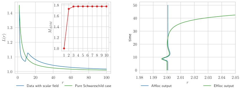
Figure 2: Left: An example of constrained solved initial data with the blue line representing data corresponding to a non-zero scalar field and the green line representing the pure Schwarzschild case. The inset plot shows the values of $M_{\textrm{ADM}}$ which are generated during the iterative solve. Right: A comparison between the output of the event horizon locator and apparent horizon locator for a simulation with a lapse perturbation in the Schwarzschild spacetime. The deviation in the two outputs at later times demonstrates the event horizon locator trying to ‘find’ the horizon. Here this effect is exaggerated because we chose a poor initial guess for the position of the event horizon on purpose.

We ask the reader to refer to Hilditch et al. (2018) for a complete derivation for the equations of motion for the optical Jacobians and only provide a brief summary of the final equations here. The evolution equations in the upper case coordinates can be written as a set of advection equations such that this subsystem is minimally coupled to the first order GHG system

$$\partial_{T}V^{-}_{\underline{i}} =(B^{\underline{j}}-AS^{\underline{j}}_{-})\partial_{\underline{j}}V^{-}_{\underline{i}}+AS^{(V^{-})}_{\underline{i}},$$

$$\partial_{T}\ln E_{-} =(B^{\underline{j}}-AS^{\underline{j}}_{-})\partial_{\underline{j}}\ln E_{-}+AS^{(E_{-})},$$ (81)

where $S^{\underline{j}}_{-}=E^{-1}_{-}V^{\underline{j}}_{-}$ and the source terms are given by

$$S^{(V^{-})}_{\underline{i}} =A^{-1}V^{-}_{\underline{j}}\partial_{\underline{i}}B^{\underline{j}}+S^{\underline{j}}{}^{\textrm{\tiny{(3)}}}\Gamma^{\underline{k}}_{\ \underline{ij}}V^{-}_{\underline{k}}$$

$$\quad-A^{-1}E_{-}\partial_{\underline{i}}A,$$

$$S^{(E_{-})} =K_{S_{-}S_{-}}-\mathcal{L}_{S_{-}}\ln A.$$ (82)

Since our objective is to evolve the optical Jacobians in the lower case ‘Cartesian’ coordinates, we must transform the evolution equations in Eqn. (III.4) using Eqns. (10) and (II). To do this, we compute $(\varphi^{-1})^{i}_{\ \underline{i}}$ which can be written down in terms of $\Phi^{i}_{\ \underline{i}}$, $\Pi^{i}$ and $V_{\underline{i}}$,

$$\left(\varphi^{-1}\right)^{i}_{\ \underline{i}}=\Phi^{i}_{\ \underline{i}}+\Pi^{i}V_{\underline{i}}.$$ (83)

The complete principal matrix $\mathbf{A}^{\underline{p}}$ associated with the GHG variables and our new variables can be expressed as

$$\mathbf{A}^{\underline{p}}=\begin{pmatrix}\Lambda_{1}&0\\ 0&\Lambda_{2}\end{pmatrix},$$ (84)

where

$$\Lambda_{1}=\begin{pmatrix}\gamma_{1}A^{-1}B^{\underline{p}}&&0&&0\\ \gamma_{2}\delta^{\underline{p}}_{\ \underline{i}}&&0&&-\delta^{\underline{p}}_{\ \underline{i}}\\ \gamma_{1}\gamma_{2}A^{-1}B^{\underline{p}}&&-{}^{\textrm{\tiny{(N)}}}\gamma^{\underline{pj}}&&0\end{pmatrix},$$ (85)

and

$$\Lambda_{2}=\begin{pmatrix}-S^{\underline{p}}_{-}&0\\ 0&-S^{\underline{p}}_{-}\end{pmatrix}.$$ (86)

Using the above expressions and Eqn. (II), the evolution equations in the lower case coordinates can be written as

$$\partial_{t}V^{-}_{\underline{i}} =(\beta^{j}-\alpha s^{j}_{-})\partial_{j}V^{-}_{\underline{i}}+\alpha W^{-1}s^{(V^{-})}_{\underline{i}},$$

$$\partial_{t}\ln E_{-} =(\beta^{j}-\alpha s^{j}_{-})\partial_{j}\ln E_{-}+\alpha W^{-1}s^{(E_{-})},$$ (87)

where

$$s^{i}_{-} =\frac{\left(\varphi^{-1}\right)^{i}_{\ \underline{i}}S^{\underline{i}}_{-}}{W\left(1+Wv_{j}\left(\varphi^{-1}\right)^{j}_{\ \underline{i}}S^{\underline{i}}_{-}\right)}+v^{i},$$ (88)

and the lower case source terms are related to the upper case sources as

$$s^{(V^{-})}_{\underline{i}} =\left(1+Wv_{j}\left(\varphi^{-1}\right)^{j}_{\ \underline{j}}S^{\underline{j}}_{-}\right)^{-1}S^{(V^{-})}_{\underline{i}},$$

$$s^{(E_{-})} =\left(1+Wv_{j}\left(\varphi^{-1}\right)^{j}_{\ \underline{j}}S^{\underline{j}}_{-}\right)^{-1}S^{(E_{-})}.$$ (89)

It is straightforward to obtain the equations of motion for the other two variables

$$\partial_{t}R=J^{\underline{0}}_{\ 0}, \partial_{t}\mathring{v}=\frac{\alpha}{W}E_{-}-b^{i}WV_{i}-b^{i}\varphi^{\underline{j}}_{\ i}V^{-}_{\underline{j}},$$ (90)

where $b^{i}=-\alpha v^{i}+\beta^{i}$. Finally, we can use the above information to construct the different components of the optical Jacobian. The $\Phi_{\ \underline{i}}^{j}$ component are evaluated in the same way as the previous case. Now

$$(J^{-1})^{\ 0}_{\underline{0}} =\partial_{T}t,$$

$$=\left(AE_{-}-B^{\underline{j}}V^{-}_{\underline{j}}\right)\chi+\mathring{v}\partial_{r}\chi\partial_{T}r-\chi\partial_{T}r$$

$$\quad-r\partial_{r}\chi\partial_{T}r-T\partial_{r}\chi\partial_{T}r+(1-\chi),$$

$$(J^{-1})^{\ i}_{\underline{0}} =\partial_{T}x^{i}=\Theta^{\underline{i}}\partial_{T}r,$$

$$(J^{-1})^{\ 0}_{\underline{i}} =\partial_{\underline{i}}t=-V_{\underline{i}}^{-}\chi+\mathring{v}\partial_{\underline{i}}\chi-(\partial_{\underline{i}}r)\chi$$

$$\quad-r\partial_{\underline{i}}\chi-T\partial_{\underline{i}}\chi,$$ (91)

where

$$\partial_{\underline{i}}\chi=(\partial_{r}\chi)\Theta^{\underline{i}}\Phi^{i}_{\ \underline{i}}.$$ (92)

The $\partial_{T}r$ term in these equations can be simplified using Eqn. (62). To initialize the evolved quantities at the beginning, we propose a choice which leads to the Jacobian being identity initially. A choice of the evolved quantities is

$$V^{-}_{\underline{i}}=-\partial_{\underline{i}}r, \mathring{v}=r, T=0.$$ (93)

The choice of $E_{-}$ is not independent but follows from the eikonal equation.

Another important point to note is that we employ the cartoon method to compute the $y$ and $z$ derivatives using Killing vectors. The formula for doing this is provided below

$$\partial_{y}V^{-}_{\underline{i}} =h(x)\left(\delta^{x}_{\ \underline{i}}\delta^{\underline{j}}_{\ y}-\delta^{y}_{\ \underline{i}}\delta^{\underline{j}}_{\ x}\right)V^{-}_{\underline{j}},$$

$$\partial_{z}V^{-}_{\underline{i}} =-h(x)\left(\delta^{x}_{\ \underline{i}}\delta^{\underline{j}}_{\ z}-\delta^{z}_{\ \underline{i}}\delta^{\underline{j}}_{\ x}\right)V^{-}_{\underline{j}}.$$ (94)

Note that $h(x)=1$ for the on-axis case and $h(x)=1/x$ otherwise.

Lastly, we briefly describe the constraint preserving outer boundary conditions, the constraint being Eqn. (80). At the outer boundary, we choose $\dot{V}^{-1}_{\underline{i}}$ to be equal to zero. This requires a choice of $\dot{E}_{-}$ which is given by

$$\dot{E}_{-}=-\frac{V_{\underline{i}}^{-}V_{\underline{j}}^{-}}{2E_{-}}{}^{\textrm{\tiny{(N)}}}\gamma^{\underline{ik}}{}^{\textrm{\tiny{(N)}}}\gamma^{\underline{jl}}\ \partial_{T}{}^{\textrm{\tiny{(N)}}}\gamma_{\underline{kl}}.$$ (95)

IV Code setup

In this section we describe our numerical setup, initial data and post-processing tools.

IV.1 Code overview

The bamps code Brügmann (2013); Hilditch et al. (2017); Bugner et al. (2016); Rüter et al. (2018) is built for large scale, parallel numerical evolutions of hyperbolic systems. Several different approximation schemes are implemented, including DG schemes Bugner et al. (2016), but here we use exclusively a multidomain pseudospectral method to solve our first order symmetric hyperbolic PDEs described in the previous sections. Each individual numerical domain is called a subpatch. Within each subpatch spatial derivatives are approximated using Chebyshev polynomials implemented, as usual, by matrix multiplication. Data are communicated between patches using a penalty method which is applied to the incoming characteristic variables at each subpatch boundary. Our domain always has a smooth timelike outer boundary at a fixed radial coordinate $r$. Because of this we need to apply boundary conditions. These need to be constraint preserving, to control undesirable gauge effects, and to control the physical behavior at the boundary Sarbach and Tiglio (2012). For now, to avoid introducing too many new complications into the code at once, we choose Jacobians that transition to the identity in a neighborhood of the outer boundary. This allows us to recycle our boundary conditions for the GHG formulation, essentially those of Rinne Rinne (2006), directly. For evolution in time we use a fourth order Runge-Kutta method. Because we will be treating spherical spacetimes we use the Cartoon method Alcubierre et al. (2001); Pretorius (2005b) to suppress two spatial dimensions. With this reduction our tests are very fast, the longest taking just a few minutes on a large desktop machine. We have tested the implementation by evolving our spherical data with the full 3d setup and obtain perfectly consistent results, and so do not discuss these slower computations further. For a deeper technical description of the code we direct the reader to Hilditch et al. (2017).

IV.2 Initial data

Our system involves a scalar field minimally coupled to the metric. To evolve such a system, we must first solve for constraint preserving initial data which can then be evolved using a combination of DF-GHG and DF scalar field projects. We shall provide the necessary coupled ordinary differential equations for the sake of completeness. Consider the coordinates $(r,\theta,\phi)$ in which the line element of the spatial metric can be written as

$$ds^{2}=l(r)^{2}dr^{2}+r^{2}d\Omega^{2},$$ (96)

where $l$ is the lower case length scalar. The form of the extrinsic curvature follows in a straightforward manner

$$K_{ij}=\begin{pmatrix}K_{rr}(r)&0&0\\ 0&r^{2}K_{T}(r)&0\\ 0&0&r^{2}\sin^{2}\theta K_{T}(r)\end{pmatrix}.$$ (97)

We can now use this to obtain the Hamiltonian and the momentum constraints which are given below respectively

$$4K_{T}K-6K_{T}^{2}+\frac{2\left(2rl^{\prime}+l^{3}-l\right)}{r^{2}l^{3}}=8\pi\left(\frac{\Phi^{\prime 2}}{l^{2}}+\Pi^{2}\right),$$

$$\frac{2\left(rK_{T}^{\prime}+3K_{T}-K\right)}{r}=8\pi\Pi\Phi^{\prime},$$ (98)

where $K$ is the trace of the extrinsic curvature, $\Phi$ is the scalar field and $\Pi$ is related to the time derivative of the scalar field as

$$\Pi=-\frac{1}{\alpha}\left(\partial_{t}\Phi-\beta^{i}\partial_{i}\Phi\right).$$ (99)

From the Hamiltonian and momentum constraints we arrive at the ODEs that we can solve using a Runge-Kutta method

$$\frac{dl}{dr} =\frac{l}{2r}\left(-2r^{2}K_{T}l^{2}K+3r^{2}K_{T}^{2}l^{2}+4\pi r^{2}l^{2}\Pi^{2}\right.$$

$$\quad\left.-l^{2}+4\pi r^{2}\Phi^{\prime 2}+1\right),$$

$$\frac{dK_{T}}{dr} =\frac{-3K_{T}+4\pi r\Pi\Phi^{\prime}+K}{r}.$$ (100)

This ODE is solved using an iterative method, with the trace of the extrinsic curvature taken to be that in Schwarzschild with the $M_{\textrm{ADM}}$ mass taken to be one. The values of $l(r)$ obtained in the first iteration is then used to construct the new ADM mass, defined by

$$M_{\textrm{ADM}}=\frac{1}{2}r\left(l(r)^{2}-1\right),\quad r\rightarrow\infty$$ (101)

This is continued until the difference between the last and the second last evaluation of the ADM mass meets a tolerance level. The spatial metric quantities can then be reconstructed using Eqn. (96), while the coordinate lightspeed $C_{+}$ constructed from

$$C_{+}=\frac{r-2M_{\textrm{ADM}}}{r+2M_{\textrm{ADM}}},$$ (102)

can be used to reconstruct the lapse and the shift

$$\alpha=\frac{l+C_{+}l}{2}, \beta_{r}=\frac{1-C_{+}}{2}.$$ (103)

An example of the initial data solver in action is shown in the left plot of Fig. 2.

IV.3 Apparent and event horizon finders

We require diagnostic tools for post-processing to ensure that the excised region of spacetime remains inside the black hole event horizon at all times during the numerical evolution. For this purpose we use two tools, the apparent horizon, defined locally on a given hypersurface and the event horizon which is a global property of the spacetime.

The apparent horizon is defined as the outermost marginally outer trapped surface on a given spatial hypersurface, that is, it is defined by the vanishing of the expansion parameter of the outgoing null geodesics. In spherical symmetry, the condition for the apparent horizon is given by Alcubierre (2008)

$$H=\frac{1}{l}\left(\frac{2}{r}+\frac{1}{\gamma_{T}}\partial_{r}\gamma_{T}\right)-2K^{\theta}_{\theta}=0,$$ (104)

where the metric is represented in the lower case basis. This is implemented in the AHloc feature of bamps. An alternative and simpler way to find the apparent horizon in the area locking coordinates is that the zero crossing of the lower case outgoing coordinate lightspeed $c_{+}$ corresponds to the position of the apparent horizon.

We will now describe the implementation of a new event horizon finder EHloc for bamps. The event horizon in general is a $2+1$ null surface which is the boundary of the black hole region from which no future pointing null geodesics can escape to null infinity $\mathcal{J}^{+}$ Hawking and Ellis (1973). Hence, one way to obtain approximations of event horizons in numerical spacetimes is to integrate null geodesics forward in time all over the numerical domain. The disadvantage of this method is that simulations can only be performed for a finite time and hence it is not straightforward to find escaping null geodesics Thornburg (2006). A more efficient algorithm is to integrate outgoing null geodesics or null surfaces backwards in time, since then the event horizon acts as an attractor of null geodesics Thornburg (2006); Diener (2003).

The geodesic method for integrating backwards in time is considered to be the most accurate method and problems mentioned in the literature like tangential drifting are not seen in practice Cohen et al. (2009). Hence, this is the method we have used for EHloc.

Unlike AHloc, it is essential for EHloc to be run in post-processing when the black hole is no longer ringing but is rather Schwarzschild. In such cases, we can start from the last numerical slice integrate the geodesic equation backwards

$$\frac{d^{2}x^{\alpha}}{d\lambda^{2}}+\Gamma^{\alpha}_{\ \beta\gamma}\frac{dx^{\beta}}{d\lambda}\frac{dx^{\gamma}}{d\lambda}=0,$$ (105)

where $\lambda$ is the affine parameter and $x^{\alpha}$ is the 4-position of the geodesic. The initial conditions for the geodesic are so chosen that it is outgoing. In spherical symmetry, the geodesic equation can be represented by a set of coupled ordinary differential equations Bohn et al. (2016)

$$\frac{d\Pi_{r}}{dt} =-\alpha_{,r}+(\alpha_{,r}\Pi^{r}-\alpha K_{rr}\Pi^{r}\Pi^{r})\Pi_{r}+\beta^{r}_{\ ,r}\Pi_{r}$$

$$\quad-\frac{1}{2}\alpha\gamma^{rr}_{\ ,r}\Pi_{r}\Pi_{r},$$

$$\frac{dr}{dt} =\alpha\Pi^{r}-\beta^{r}.$$ (106)

Here $\alpha$, $\beta^{i}$ are the lapse and shift respectively, $K_{ij}$ is the extrinsic curvature and $\gamma^{ij}$ is the inverse of the spatial metric. All quantities mentioned here are represented in the lower case basis. The intermediate variable $\Pi_{r}$ is related to the momentum $p_{r}=dx_{r}/d\lambda$ as

$$\Pi_{r}\equiv\frac{p_{r}}{\sqrt{\gamma^{ij}p_{i}p_{j}}}.$$ (107)

A Runge-Kutta integrator is used for performing the time stepping while the data is loaded and then interpolated using Chebyshev functions. A brief description of the grid and interpolation setup is given below.

The data is written on every patch at the Gauss-Lobatto points

$$x_{\alpha}=-\cos\left(\frac{\pi\beta}{N-1}\right),$$ (108)

where $N$ is the number of points on each grid and $\beta=0,\ldots,N-1$. Chebyshev polynomials are used to perform the spectral interpolation

$$T_{n}(x)=\cos(n\cos^{-1}x).$$ (109)

These polynomials are defined in the interval $[a,b]$ by a change of variable:

$$y\equiv\frac{x-\frac{1}{2}(b+a)}{\frac{1}{2}(b-a)}.$$ (110)

The coefficients of interpolation $a_{0},\ldots,a_{n-1}$ are found out by solving:

$$\begin{pmatrix}T_{0}(x_{0})&\dots&T_{N-1}(x_{0})\\ \vdots&\ddots&\\ T_{0}(x_{n-1})&&T_{N-1}(x_{N-1})\end{pmatrix}\begin{pmatrix}a_{0}\\ \vdots\\ a_{N-1}\end{pmatrix}=\begin{pmatrix}u_{0}\\ \vdots\\ u_{N-1}\end{pmatrix},$$ (111)

where $u_{0},\ldots,u_{N-1}$ are the given values at the $N$ points. The spatial derivatives are computed by a matrix multiplication Hilditch et al. (2016):

$$(\partial_{x}u)_{\alpha}=\sum^{N-1}_{k=0}D_{\alpha k}u_{k},$$ (112)

where $D_{\alpha\beta}$ is the Gauss-Lobatto derivative matrix given by

$$D_{\alpha\beta}=\begin{cases}\frac{-2(N-1)^{2}+1}{6},\ \alpha=\beta=0,\\ \frac{q_{\alpha}(-1)^{\alpha+\beta}}{q_{\beta}(x_{\alpha}-x_{\beta})},\ \alpha\neq\beta,\\ -\frac{x_{\beta}}{2(1-x^{2}_{\beta})},\ \alpha=\beta=1,\ldots,N-1,\\ \frac{2(N-1)^{2}+1}{6},\ \alpha=\beta=N-1,\end{cases}$$ (113)

where $q_{\alpha}=2$ at the boundary points and $q_{\alpha}=1$ elsewhere.

In practice, we do not compute the diagonal terms of the derivative matrix but use the identity which gives the derivative matrix better stability against rounding errors

$$D_{\alpha\alpha}=-\sum^{N-1}_{k=0,k\neq\alpha}D_{\alpha k}.$$ (114)

The time interpolation on the data is performed using a linear interpolation algorithm and a judicious choice of the number of points needs to be taken into account. The number of data steps loaded into memory also affects performance. However, both of these problems are hardware specific and hence we do not go into details here. As sanity checks, we test the event horizon finder with a multi-patch simulation of the Schwarzschild spacetime and another with a gauge perturbation. These results have also been compared with the output of the apparent horizon finder and seen to be in good agreement. The gauge perturbation case with both EHloc and AHloc outputs are shown in the right plot of Fig. 2.

V Numerical results

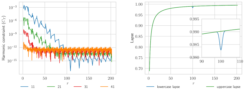
Figure 3: Left: A convergence test performed with the time component of the harmonic constraints when the analytic Jacobian given in Eqn. (37) is considered. The numbers in the legend correspond to the number of points per patch considered. Right: A comparison between the lower case and the upper case lapse at time $t\simeq 5$ for the same set of simulations.

V.1 Tests with analytic Jacobians

We begin our numerical experiments by first testing out our implementation of the analytic Jacobians. As initial data, we choose the metric components to be those of the Schwarzschild spacetime in Kerr-Schild coordinates. We perform simulations for both the analytic Jacobians keeping the function $f$ to be

$$f=1+0.0001t^{2}e^{-(r-100)^{2}}e^{-(t-5)^{2}}.$$ (115)

The numerical domain for these simulations are from $r\in[1.8,201.8]$ and they are performed at $4$ different resolutions starting from $20$ patches, $11$ points and increasing the number of points by $10$ in each case. We finally plot the harmonic constraints

$$C_{\underline{\alpha}}=H_{\underline{\alpha}}+g^{\underline{\beta\gamma}}\ \Gamma_{\underline{\alpha\beta\gamma}},$$ (116)

with radius at four different resolutions and find that the constraints converge with increasing resolution. A plot of such a convergence test is provided in Fig. 3. We also perform tests of the time derivatives of the harmonic constraints given by

$$F_{\underline{\alpha}}\simeq\partial_{N}H_{\underline{\alpha}}+g^{\underline{\beta\gamma}}\partial_{N}\Gamma_{\underline{\alpha\beta\gamma}}-\Gamma_{\underline{\alpha}}^{\ \underline{\beta\gamma}}\partial_{N}g_{\underline{\beta\gamma}},$$ (117)

where $\simeq$ denotes equality up to the combinations of the reduction constraints and $\partial_{N}\equiv N^{\underline{\alpha}}\partial_{\underline{\alpha}}$ (see Lindblom et al. (2006); Hilditch et al. (2016) for details). We find that they also converge with increasing resolution.

V.2 Tests with the vanishing shift Jacobian

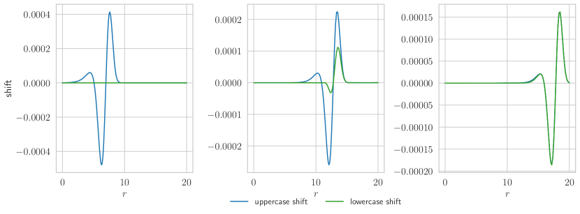
Figure 4: A snapshot of the upper case shift and the lower case shift at three different times given by $t\simeq 7.7$, $13.5$ and $18.5$ (in units of $M$). In the first figure, we see as expected irrespective of the upper case shift, the lower case shift is vanishingly small inside the transition region. In the second figure, we demonstrate the effect of the transition region on the lower case shift. In the third figure, we see the form of the lower case shift mostly outside the transition region where it is expected to agree with its upper case counterpart.

Another numerical experiment we perform is to keep the lower case shift to be zero by a suitable choice of Jacobian. This experiment is performed on the Minkowski spacetime by adding a Gaussian gauge wave of the form

$$\alpha =1+G^{\prime}e^{-w^{\prime}(r-r_{0})^{2}},$$ (118)

where the parameters of the perturbation are given by

$$G^{\prime}=0.2, r_{0}=0, w^{\prime}=1.$$ (119)

As has been demonstrated in the calculations of section III, the upper case and the lower case coordinates match in the outermost subpatch of the simulation while the penultimate subpatch serves as the transition region. This can be seen clearly in the plots in Fig. 4 where the upper case shift is represented by the blue curve and the lower case shift is represented by the green curve. The lower case shift is successfully kept to zero in patches inside the transition zone, while outside the transition zone, it is seen to agree with the upper case shift. A convergence test is also performed considering the reduction constraints, the harmonic constraints and the time derivatives of the harmonic constraints and we see convergence with increase in resolution, as is expected.

V.3 Tests with the areal radius Jacobian

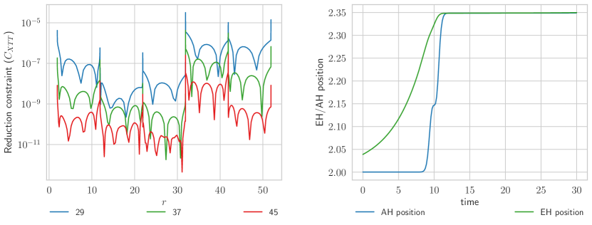
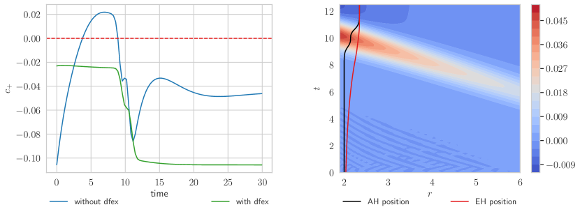
Figure 5: Top row, left: A convergence test performed with the $XTT$ component of the reduction constraints at $t=30M$ performed at three different resolutions, the number of points per patch being mentioned in the legend. These simulations are performed with the GHG, DF and scalar field projects. Top row, right: The position of the apparent horizon and the event horizon as a function of time in one of these simulations with DF, GHG and scalar field. The position of the apparent horizon, also where $c_{+}$ crosses zero is seen to increase monotonically as a function of time. Bottom row, left: A plot showing the value of the outgoing radial coordinate lightspeed $c_{+}$ at the inner boundary of two simulations, one performed with DF-excision and another performed without it. The simulation performed with DF-excision switched on has a negative value of $c_{+}$ at the inner boundary throughout the simulation while the non-DF simulation fails in maintaining that. Bottom row, right: The time evolution of the scalar field along with the position of the event horizon and the apparent horizon.

We now perform simulations of a massless scalar field minimally coupled to general relativity in spherical symmetry. As a first try, we evolve the spacetime in generalized harmonic coordinates Lindblom et al. (2006) using the old excision setup, that is, there are no boundary conditions placed at the inner boundary which is expected to be outflow at the beginning of the simulation. We also monitor the signs of the two radial coordinate lightspeeds as given in Eqn. (75) at the inner boundary of the simulation at all times. We set the scalar field data initially to be of the following profile

$$\Phi =\frac{C}{r}e^{-(r-r_{0})^{2}/\sigma^{2}},$$

$$\Pi =-\frac{2C}{r\sigma^{2}}(r-r_{0})e^{-(r-r_{0})^{2}/\sigma^{2}}.$$ (120)

The specific parameters which are chosen for the run are

$$C=0.1, r_{0}=11.9, \sigma=1.$$ (121)

Using these parameters, we then solve for the spatial metric, extrinsic curvature, lapse and shift in the initial data using the method prescribed in section IV.2.

A plot of the outgoing radial coordinate lightspeed $C_{+}$, as can be seen in the bottom row, left of Fig. 5 shows that it assumes a positive sign at the inner boundary for some time during the simulation. This indicates that the excision strategy has failed as the inner boundary has not remained an outflow boundary during those times. This experiment clearly demonstrates that for certain configurations of the matter content, the existing excision strategy is unsuccessful.

We now perform the same experiment, but this time we switch on DF and the areal radius Jacobian as described in section III. As described before, the use of the areal radius ensures that the position of the apparent horizon can only monotonically increase with time, which ensures that if it is initially located inside the numerical domain, it shall do so at all times. Like before, the lightspeeds at the inner boundary are monitored at all times. It can be clearly seen, from the green line in the bottom left of Fig. 5 that the value of $C_{+}$ at the inner boundary remains negative at all times during the simulation thereby indicating that the new excision strategy is successful. Although not seen in the plot, the $C_{-}$ lightspeed, while its value fluctuates, remains negative at all times for both the DF and the non-DF case. This fact can be seen from Eqn. (75) which shows that if $C_{+}$ remains negative at all times, so must the value of $C_{-}$. We also perform simulations with different quantities of scalar field content and find many other cases where the new method proves to be successful where the old one does not.

With the parameters which have been provided above, we perform simulations at three different resolutions, having $29$, $37$ and $45$ points per patch and plot the reduction constraints which are defined by (15) and can be computed in the lower case coordinates from

$$C_{\underline{i\alpha\beta}}=\left(\varphi^{-1}\right)^{k}_{\ \underline{i}}\partial_{k}g_{\underline{\alpha\beta}}+V_{\underline{i}}\Pi_{\underline{\alpha\beta}}-\Phi_{\underline{i\alpha\beta}},$$ (122)

as a function of space for a given value of time. We see convergence with increase in resolution, as can be seen in the top left plot of Fig. 5.

We also employ our event horizon and apparent horizon finders to track the location of the horizons. A superposition of the output of the two finders is provided at the top right of Fig. 5. As expected the apparent horizon grows monotonically with time from $2M$ to $\simeq 2.35M$. The event horizon also shows a monotonic behavior in these coordinates.

Another experiment we perform involves evolving the Schwarzschild spacetime with a lapse perturbation

$$\alpha =\alpha^{\prime}+H^{\prime}e^{-w^{\prime}(r-r_{0})^{2}},$$

$$\partial_{i}\alpha =\partial_{i}\alpha^{\prime}-2H^{\prime}w^{\prime}(r-r_{0})e^{-w^{\prime}(r-r_{0})^{2}}\frac{x_{i}}{r},$$ (123)

where $\alpha^{\prime}$ is the natural lapse associated with the Schwarzschild metric in Kerr-Schild coordinates. The specific parameters which are chosen for this experiment are

$$H^{\prime}=1, r_{0}=10, w^{\prime}=1.$$ (124)

The lapse perturbation is shown in the inset plot of Fig. 6. We observe the zero crossing of the outgoing radial coordinate lightspeed $C_{+}$ as this corresponds to the position of the apparent horizon. At the beginning of the simulation, this stays at $2M$ and continues to remain so throughout the entire duration of the simulation. This is shown by the blue and green lines in the left plot of Fig. 6 which correspond to the lightspeed at the beginning and at the end of the simulation. This is indeed the desired behavior since the position of the apparent horizon should not change as there is no physical perturbation.

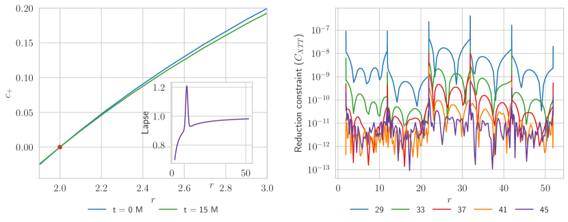
Figure 6: Left: A demonstration of the fact that the position of the apparent horizon does not change when hit by a lapse perturbation. In the figure, the outgoing radial coordinate lightspeed $c_{+}$ is shown at two different times and it is seen that the zero crossing remains at $2M$ throughout the simulation. The inset plot shows the lapse perturbation in the initial data. Right: A convergence plot of the $XTT$ component of the reduction constraints performed with five different resolutions of the same lapse perturbation simulation. The legend shows the number of points per patch.

V.4 Tests with the DF-excision Jacobian

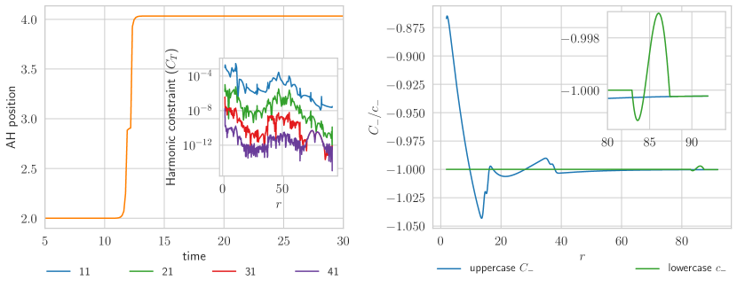
Figure 7: Left: A demonstration showing the growth of the apparent horizon by $\simeq 101\%$ by accreting scalar field into the black hole. The inset plot shows a convergence test with the time component of the harmonic constraint. The legend shows the number of points per patch. Right: A plot of the incoming radial coordinate lightspeed $C_{-}/c_{-}$ in both the upper case and the lower case coordinates with the lower case result shown to be $-1$ inside the transition region. The inset plot zooms in on the transition region and shows that the upper case and lower case speeds agree at the outermost subpatch.

Finally, we perform numerical experiments with the dual foliation eikonal Jacobian. The numerical setup again consists of a massless scalar field minimally coupled to general relativity. Control of the $C_{+}$ radial coordinate lightspeed is borrowed from the treatment in the previous section. In this section, our goal is also to control the ingoing radial coordinate lightspeed $C_{-}$ to be identically $-1$ inside the transition region. This would prevent any redshift or blueshift of the scalar field pulse as it falls into the event horizon. We prepare initial data using our initial data solver for scalar field of the type given by Eqn. (V.3) with the parameters given by

$$C=0.21, r_{0}=15, \sigma=1.$$ (125)

Our principal objective in this experiment is to grow the apparent horizon as much as possible by letting accreting scalar field fall into the black hole horizon. For this specific choice of parameters, we see that the apparent horizon position grows from $\simeq 2M$ to $4.03M$ thereby registering $\simeq 101\%$ increase. This increase, which is monotonic with time is demonstrated clearly in the left plot of Fig. 7. We also perform convergence tests by considering simulations with $11$, $21$, $31$ and $41$ points per patch and with each simulation containing $10$ patches. Plots of the reduction constraints, harmonic constraints and the time derivatives of the harmonic constraints all demonstrate convergence with increasing resolution as is expected. As a demonstration, the inset plot of the right hand side of Fig. 7 shows the convergence of the harmonic constraints.

Finally, we look at the outgoing radial coordinate lightspeed in both the upper case and the lower case coordinates, as can be seen from the right plot of Fig. 7. The upper case $C_{-}$ is seen to vary freely while our method ensures that the lower case $c_{-}$ is strictly kept to be equal to $-1$ throughout the entire simulation inside the transition region. As can be seen from the inset plot of the same figure, the two lightspeeds disagree in the transition patch but they do agree in the outermost patch as expected.

VI Conclusions

In this paper, we have presented the first implementation of the DF-GHG formulation, together with the DF-scalar field. The implementation was made within the bamps code. We performed a battery of tests involving several Jacobians, but with an emphasis on black hole excision. Although the tests performed are in spherical symmetry as proof of concept and also for reasons of efficiency, the whole implementation itself was made in the full $3+1$ setting. In addition to this, we introduced our event horizon finding code EHloc.

To test the newly written DF-GHG project, we have performed elementary tests with two analytic Jacobians, in one of which we consider two different foliations for the upper case and lower case coordinates. After this, we tested the vanishing shift Jacobian, another important case in which the lower case shift is kept zero at all times, which we expect to be helpful while considering cases of gravitational collapse and black hole formation.

Finally, we considered the two most important Jacobians for our black hole excision work, the areal radius Jacobian and the DF-excision Jacobian. In the areal locking case, we saw that when the lower case coordinates are made to include the areal radius, the apparent horizon is located at the zero-crossing of the outgoing radial coordinate lightspeed $c_{+}$. By basic results for dynamical horizons, these coordinates also have the special property that the position of the apparent horizon cannot decrease. Thus if the apparent horizon is initially located on the numerical grid, it stays so throughout the simulation. Assuming the weak cosmic censorship conjecture, we then ensure that the event horizon, being located outside the apparent horizon, also remains on the numerical grid. In the case of the DF-excision Jacobian, we carefully control the ingoing radial coordinate lightspeed $c_{-}$ to be equal to $-1$ identically while enforcing the previous condition for the outgoing speed. Controlling $c_{-}$ to be a constant everywhere on the numerical grid, barring the transition region and outside, ensures that the redshift or blueshift that potentially arises out of using ‘artificial’ coordinates is avoided. We performed a series of tests on the Minkowski spacetime with lapse perturbations or perturbed Schwarzschild spacetimes by employing a combination of the DF, DF-GHG and DF-scalarfield projects. These tests were validated by performing several convergence tests, which demonstrate clean spectral convergence.

The excision setup presented here is of course highly specialized when compared with the full control system approach used in the SpEC code. That said it provides precisely the functionality needed for our near-term work, and has the advantage that we use only pointwise, rather than quasilocal manipulation of our variables in constructing the Jacobians. Therefore, at the continuum level, basic theorems can be trivially applied to our formulation. To avoid coupling through derivatives between the Jacobian and evolution equations, which would require a more careful mathematical analysis, it was crucial that we could replace first derivatives of the metric using the reduction constraints. This works because the expansion contains at most one derivative of the metric. Since this fact remains true even in the absence of spherical symmetry we hope, eventually, to generalize the DF-excision strategy to the full $3+1$ setting. For now it is unclear whether or not this will pan out, since there is a qualitative difference between 1d and 3d excision that cannot be overlooked. But if successful the generalization would provide an improved moving excision strategy for binary black holes within a pseudospectral code.

In order to perform our numerical tests, appropriate boundary conditions at the outer boundary must be provided. At present, we do not yet have outer boundary conditions in the code for the DF projects. To overcome this problem at the outer boundary, we ensure that the Jacobian transitions into the identity Jacobian at the outermost subpatch. This is achieved by using a low order polynomial transition function, which works remarkably well in practice when the transition is placed at the two ends of the penultimate subpatch, and we expect that various alternative configurations would behave similarly. A desirable alternative would be to implement outer boundary conditions in the code that take care of the full DF infrastructure, including the management of two time coordinates. Work on this will be reported on in the near future. An immediate goal is to use the methods developed here to study systematically, in the spherical context, the transition from the linear regime we studied in Bhattacharyya et al. (2020) to the case with arbitrary non-linear perturbations.