Phonon Self-Energy Effects in Migdal-Eliashberg Theory

Abstract

Recent work on an electron-phonon model in two-dimensions is reviewed and some new results are presented. We utilize both Quantum Monte Carlo simulations and Migdal-Eliashberg theory. The type of electron-ion coupling considered is on-site. Competing instabilities are charge density wave (CDW) and singlet superconductivity. When the electron band is half-filled, the charge density wave dominates. Away from half-filling CDW correlations actually suppress superconductivity.

I introduction

The discovery of high temperature superconductivity has motivated renewed interest in the question of competing instabilities and their relation to superconductivity. In particular, in most of the cuprates the phase diagram shows an antiferromagnetic and superconducting ground state in close proximity to one another. Even earlier, it had been noted that a charge density wave (CDW) and superconducting ground state competed with one another in BaPb_1-xBi_xO₃. Such competition between various non-Fermi liquid-like ground states has been a recurrent theme in A-15, organic and heavy fermion materials.

In this paper we do not wish to address specifically any of the materials mentioned above. Instead, we wish to consider a highly idealized model and investigate in particular the competition between superconductivity and a charge density wave. The model under consideration is the Holstein (or molecular crystal) model with Hamiltonian:

$$H = -\sum_{{\langle ij\rangle}\atop\sigma}t_{ij}(c^{\dagger}_{i\sigma}c_{j\sigma}+c^{\dagger}_{j\sigma}c_{i\sigma})-\mu\sum_{i\sigma}n_{i\sigma}$$ (1)

$$+ \sum_{i}\left({p_{i}^{2}\over 2M}+{1\over 2}Kx_{i}^{2}\right)-\alpha\sum_{i\sigma}x_{i}(n_{i\sigma}-{1\over 2})$$

where $x_{i}$ and $p_{i}$ are scalar position and momentum operators for the ion with mass $M$ and spring constant $K$ ($=M\omega_{E}^{2}$) at site $i$. $c^{\dagger}_{i\sigma}$ is the creation operator for an electron with spin $\sigma$ at site $i$. Hopping occurs via the first term in the Hamiltonian, with probability amplitude $t_{ij}$. In this paper, this summation will be restricted to $i$ and $j$ nearest neighbours only. The chemical potential, $\mu$, is chosen to give a set number density of electrons, $n$. The last term couples the electron density $n_{i\sigma}\equiv c^{\dagger}_{i\sigma}c_{i\sigma}$ with the lattice displacement, $x_{i}$ at site $i$, with coupling constant $\alpha$.

A variety of techniques has been used to treat the Hamiltonian in Eq. (1), most notably, in recent years, Quantum Monte Carlo simulation. Hirsch and Fradkinhirsch82 investigated the one dimensional case. The two dimensional case has been investigated by Scalettar er al.,scalettar89 Levine and Sulevine90 and the author.marsiglio89 Perturbation theory has also been used and will be further discussed in this paper. The idea is to approach any pending phase transition from high temperature and to determine the susceptibilities for either singlet pairing or charge density wave formation. Other approaches are also possible, such as varying the chemical potential (occupation) or, less physically, the coupling constant, $\alpha$. Here we review the two dimensional work which has been done including some very recent work by Noack et al.scalettar89 The strategy is to simulate the Hamiltonian (1) on a small square lattice ($4\times 4$) while at the same time we solve the equations arising from self-consistent perturbation theory on the same size lattice with the same boundary conditions (in this case, periodic). By comparing susceptibilities we get a quantitative measure of the accuracy of our perturbative approximation, which can then be evaluated in the thermodynamic limit. In the following we use units such that $\hbar=k_{B}=1$.

II Theoretical Background

The Monte Carlo algorithm used is that of Blankenbecler et al.blankenbecler81 with modifications due to Hirschhirsch88 to give greater stability at lower temperature. We have used the Monte Carlo results primarily as benchmarks with which to guide our perturbative calculations.

The perturbative approach is summarized diagrammatically in Fig. 1. The one-electron Green’s function is given by

$$G(\vec{k},i\omega_{m})=[i\omega_{m}-(\epsilon_{k}-\mu)-\Sigma(\vec{k},i\omega_{m})]^{-1}$$ (2)

where $i\omega_{m}\equiv i\pi T(2m-1)$ are the fermion Matsubara frequencies, and $\epsilon_{k}$ is the single particle energy obtained from diagonalizing the first term in the Hamiltonian (1). The self-energy due to the electron-phonon interaction is given by $\Sigma(\vec{k},i\omega_{m})$. Similarly the phonon propagator is given by

$$D(\vec{q},i\nu_{m})=[-M(\omega_{E}^{2}+\nu_{n}^{2})-\Pi(\vec{q},i\nu_{n})]^{-1}$$ (3)

where $i\nu_{n}\equiv 2i\pi Tn$ are the boson Matsubara frequencies, and $\omega_{E}$ is the Einstein phonon frequency. In this model, because we have used a site-diagonal coupling, the unperturbed phonon frequency has no dispersion. Finally $\Pi(\vec{q},i\nu_{n})$ is the phonon self-energy due to the electron-phonon interaction. Migdalmigdal58 originally argued that $\Pi(\vec{q},i\nu_{n})$ led to a renormalization of the phonon frequency $\omega_{E}\rightarrow\Omega(\vec{q})$. In practice the phonon spectrum is often taken from experiment, so that the calculation of $\Pi(\vec{q},i\nu_{n})$ is not required. Here, since we wish to predict pending instabilities, it is necessary to retain $\Pi(\vec{q},i\nu_{n})$ explicitly.

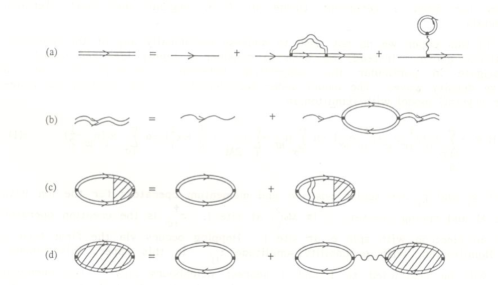
Figure 1: Fully self-consistent equations for (a) the interacting electron propagator (straight double lines), (b), the interacting phonon propagator (wavy double line), (c) the singlet pairing susceptibility in the “ladder” approximation, and (d) the CDW susceptibility in the “bubble” approximation. Single lines represent non-interacting propagators.

The approximations indicated in Figs. 1a,b are:

$$\Sigma(\vec{k},i\omega_{m}) = {\alpha^{2}\over N\beta}\sum_{k^{\prime},m^{\prime}}D(\vec{k}-\vec{k^{\prime}},i\omega_{m}-i\omega_{m^{\prime}})G(\vec{k^{\prime}},i\omega_{m^{\prime}})\phantom{aaa}$$ (4)

$$\Pi(\vec{q},i\nu_{n}) = {2\alpha^{2}\over N\beta}\sum_{k,m}G(\vec{k},i\omega_{m})G(\vec{k}+\vec{q},i\omega_{m}+i\nu_{n}).$$ (5)

In addition, the occupancy requirement is

$$n={2\over N\beta}\sum_{k,m}G(\vec{k},i\omega_{m})e^{i\omega_{m}0^{+}}$$ (6)

which determines the chemical potential, $\mu$. Here $\beta\equiv 1/T$. There are no vertex corrections in Eqs. (4) and (5). However, Eqs.(2-5) form a set of fully self-consistent equations in two dimensional momentum and one dimensional frequency space, for the electron and phonon propagators. We have demonstrated the need for self-consistently at half-filling previously.marsiglio89 The singlet pairing (SP) and CDW susceptibilities are given by:hirsch85

$$\chi^{\rm SP} = {1\over N}\sum_{ij}\int_{0}^{\beta}d\tau\langle c_{i\uparrow}(\tau)c_{i\downarrow}(\tau)c^{\dagger}_{j\downarrow}(0)c^{\dagger}_{j\uparrow}(0)\rangle$$ (7)

$$\chi^{\rm CDW}(\vec{q}) = {1\over N}\sum_{{ij}\atop\sigma\sigma^{\prime}}e^{i\vec{q}\cdot(\vec{R}_{i}-\vec{R}_{j})}\int_{0}^{\beta}d\tau\left[\langle n_{i\sigma}(\tau)n_{j\sigma^{\prime}}(0)\rangle-\langle n_{i\sigma}(\tau)\rangle\langle n_{j\sigma^{\prime}}(0)\rangle\right].$$ (8)

These susceptibilities are measured directly in the Monte Carlo simulations. In the approximations given in Fig. 1, they are given by

$$\chi^{\rm SP}={1\over N\beta}\sum_{k,m}F(\vec{k},i\omega_{m})\Lambda(\vec{k},i\omega_{m})$$ (9)

and

$$\chi^{\rm CDW}(\vec{q})={\bar{\chi}^{\rm CDW}(\vec{q})\over 1-\lambda_{0}\bar{\chi}^{\rm CDW}(\vec{q})}$$ (10)

where

$$F(\vec{k},i\omega_{m})=G(\vec{k},i\omega_{m})G(-\vec{k},-i\omega_{m}),$$ (11)

$$\bar{\chi}^{\rm CDW}(\vec{q})=-{1\over\alpha^{2}}{\rm Re}[\Pi(\vec{q},0)]$$ (12)

and

$$\lambda_{0}\equiv{\alpha^{2}\over M\omega_{E}^{2}}.$$ (13)

$\Lambda(\vec{k},i\omega_{m})$ is the solution of the vertex equation:

$$\Lambda(\vec{k},i\omega_{m})=1-{\alpha^{2}\over N\beta}\sum_{k^{\prime}m^{\prime}}F(\vec{k}^{\prime},i\omega_{m^{\prime}})D(\vec{k}-\vec{k}^{\prime},i\omega_{m}-i\omega_{m^{\prime}})\Lambda(\vec{k}^{\prime},i\omega_{m^{\prime}}).$$ (14)

Equation (14) with the “1” removed simply becomes the Eliashberg equation to determine $T_{c}$. Once again iteration is required in two dimensional momentum and one dimensional frequency space.

The importance of including the phonon self-energy, $\Pi(\vec{q},i\nu_{n})$ in Eq. (3) is apparent upon inspection of Eq. (12). In effect we are including the CDW correlations into the one-electron Green’s function. In what follows we will call the approximation which includes $\Pi(\vec{q},i\nu_{n})$ the “renormalized Migdal-Eliashberg approximation,” and the one which omits $\Pi(\vec{q},i\nu_{n})$ the “unrenormalized Migdal-Eliashberg approximation.”

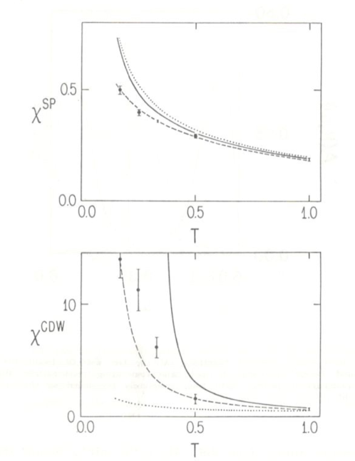
Figure 2: Plot of (a) $\chi^{\rm SP}$ and (b) $\chi^{\rm CDW}(\vec{q}=(\pi,\pi))$ vs. temperature for a $4\times 4$ lattice, with $\lambda_{0}=1.5$ and $\omega_{E}=0.5$, at half-filling. Points are from Monte Carlo simulations, dashed lines from the renormalized Migdal-Eliashberg approximation and solid lines from the unrenormalized Migdal-Eliashberg approximation. Including the phonon self-energy self-consistently gives far better agreement with the Monte Carlo results. The non-interacting limit (dotted lines) is included for comparison.

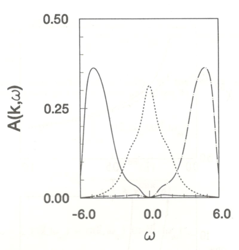
Figure 3: Plot of the spectral function $A(\vec{k},\omega)$ for $\vec{k}=(0,0)$ (solid line), $\vec{k}=(\pi/2,\pi/2)$ (dashed line) and $\vec{k}=(\pi,\pi)$ (dot-dashed line) calculated using renormalized Migdal-Eliashberg theory. The quasiparticle peaks have been completely broadened so that the spectra are entirely incoherent ($\lambda_{0}=2$, $\omega_{E}=1$, $n=1$).

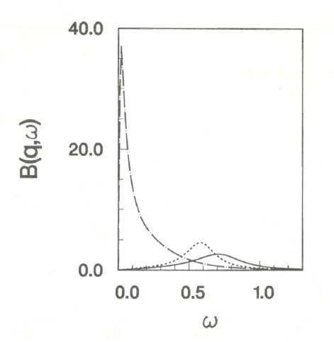
Figure 4: Plot of the phonon spectral function $B(\vec{q},\omega)$ for $\vec{q}=(0,0)$ (solid line), $\vec{q}=(\pi/2,\pi/2)$ (dashed line) and $\vec{q}=(\pi,\pi)$ (dot-dashed line) calculated within the renormalized Migdal-Eliashberg approximation for the parameters of Fig. 3. The unperturbed phonon frequency is $\omega_{E}=1.0$. Considerable dispersion has developed, along with mode softening and broadening. The CDW instability is imminent as the $\vec{q}=(\pi,\pi)$ mode has softened to nearly zero frequency.

III Half-filling

The situation at half-filling was investigated in Ref. [marsiglio89, ], and also recently by Noack et al.scalettar89 We reproduce in Fig. 2 the pairing and CDW susceptibilities as a function of temperature, taken from Ref. [marsiglio89, ]. Here $\lambda_{0}=1.5$ and $\omega_{E}=0.5$, in units of the nearest neighbour hopping matrix element, $t$, and we have used a $4\times 4$ lattice. It is clear that (a) CDW correlations dominate, and (b) the renormalized Migdal-Eliashberg approximation is required for an accurate quantitative description. In Fig. 3 we plot the electron spectral function, $A(\vec{k},\omega)\equiv-{\rm Im}G(\vec{k},\omega+i\delta)/\pi$, calculated using Eqs. (2-6) versus frequency for several values of momentum. The analytic continuation was determined by using Padé approximants.vidberg77 Most noteworthy is the spectral function for $\vec{k}=(\pi/2,\pi/2)$ which is on the Fermi surface, where the spectral function has become entirely smeared out over an energy range of order the original bandwidth. This fact remains for larger lattice sizes as well. This is to be contrasted with the spectral function computed using $\Pi(\vec{q},i\nu_{n})=0$. In the latter case the quasi-particle peak remains intact (see Ref. [marsiglio89, ]), with only a small amount of spectral weight transferred to regions a (unperturbed) phonon frequency away. This is due to the fact that information of the imminent CDW transition has not been included in the one-electron spectral function in this approximation. It is thus no longer useful to compute a mass enhancement given by $\lambda_{k}\equiv-\partial{\rm Re}\Sigma(\vec{k},\omega)/\partial\omega|_{\omega=E_{F}}$. In Fig. 4 we illustrate the phonon spectral function, $B(\vec{q},\omega)\equiv-{\rm Im}D(\vec{q},\omega+i\delta)/\pi$, for positive frequency for various wave-vectors. Clearly the original Einstein mode has acquired dispersion with some broadening with the zone corner mode softening nearly to zero frequency. This is another signal that a $\vec{q}=(\pi,\pi)$ CDW instability is occurring.

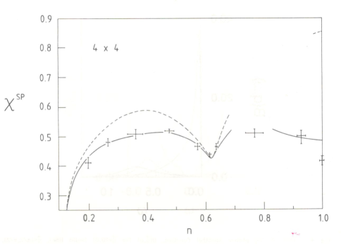
Figure 5: Plot of the singlet pairing susceptibility, $\chi^{\rm SP}$ vs. occupation, $n$, for a $4\times 4$ system ($\lambda_{0}=2$, $\omega_{E}=1$, and $\beta=6$). The points with error bars are the Monte Carlo results, the solid line was obtained using renormalized Migdal-Eliashberg theory ($\Pi(\vec{q},i\nu_{n})\neq 0$) and the dashed line was obtained using unrenormalized Migdal-Eliashberg theory ($\Pi(\vec{q},i\nu_{n})=0$). Note the considerable improvement due to phonon renormalization, particularly near half-filling. Portions of the curves are missing due to the fact that the equations would not converge due to the finite size of the system. At half-filling the unrenormalized susceptibility vastly overestimates the true result.

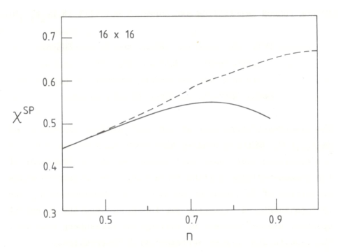
Figure 6: Plot of the singlet pairing susceptibility vs. occupation for the same parameters as in Fig. 5 but for a much larger system size ($16\times 16$ ), which is representative of the bulk. At low fillings CDW correlations are not present. As the filling approaches 1, the system actually undergoes a transition to a CDW, so that the renormalized Migdal-Eliashberg equations are unable to converge. (They predict a transition near $n=0.88$ at $\beta=6$.) It is clear that the strong CDW correlations actually suppress the SP susceptibility at intermediate concentrations.

IV Away from half-filling

At half-filling, the CDW correlations always dominate over the SP correlations. Away from half-filling, the perfect nesting in this model (we have taken nearest neighbour hopping only) is destroyed and eventually a transition to a superconducting state is expected. The question then arises:levine90 ; scalettar89 to what extent do CDW correlations enhance or suppress superconductivity? At very low fillings, CDW correlations are absent, and hence play no role in superconductivity. At intermediate densities, however, they are expected to have some effect. A suitable test for this hypothesis is to compare our Green’s functions calculation with and without CDW correlations with Monte Carlo results. As already discussed this is achieved by including or omitting $\Pi(\vec{q},i\nu_{n})$ in the calculation, respectively. The result for a $4\times 4$ lattice is shown in Fig. 5. Here, $\lambda_{0}=2.0$, $\omega_{E}=1.0$ and $\beta=6$. $\chi^{\rm SP}$ is plotted as a function of density, $n$, obtained by i) Monte Carlo simulation (points with error bars), ii) the fully self-consistent Green’s function calculation with $\Pi(\vec{q},i\nu_{n})$ included (solid line) , and iii) the Green’s function calculation with $\Pi(\vec{q},i\nu_{n})$ set equal to zero (dashed line). Finite size effects are quite significant, so all calculations are done on a $4\times 4$ lattice, with periodic boundary conditions. While there is some difficulty in obtaining convergence near half-filling for the calculations, due to the small system size, it is clear that including CDW correlations in the Green’s function calculation provides far better agreement with the Monte Carlo results. This gives us confidence that including $\Pi(\vec{q},i\nu_{n})$ improves the approximation. We also take this as a strong indication that CDW correlations influence the pairing susceptibility, and in fact suppress it. It is difficult to verify this for much larger lattices, because of the computation time required for the simulations. However, in Fig. 6 we show the pairing susceptibility for the same parameters as before, but for a $16\times 16$ lattice, calculated by the two perturbative theories. For $\beta=6$, this size lattice is representative of the bulk. Note that in the lower occupation regime in which there previously was a suppression in $\chi^{\rm SP}$ (see Fig. 5) the two calculations now give essentially the same result. Nonetheless, at occupations closer to half-filling there is clearly a suppression of $\chi^{\rm SP}$ brought on by the CDW correlations. Unfortunately we do not have the Monte Carlo data for a $16\times 16$ lattice to verify this. However, based on the success of the renormalized Migdal-Eliashberg result in the $4\times 4$ case (Fig. 5), Fig. 6 suggests that CDW correlations suppress the superconducting susceptibility.

V summary

Through a combination of Quantum Monte Carlo simulations on small 2-D systems and fully self-consistent Green’s function calculations using the Migdal-Eliashberg approximation, we conclude that in this model i) at half-filling the ground state is a CDW with ordering wave-vector $\vec{q}=(\pi,\pi)$, ii) while we have not explicitly demonstrated it here, the ground state at sufficient doping levels away from half-filling will be superconducting, and iii) for concentrations near half-filling the residual CDW correlations actually suppress the SP susceptibility.