Autoregressive Denoising Diffusion Models for Multivariate Probabilistic Time Series Forecasting

Abstract

In this work, we propose TimeGrad, an autoregressive model for multivariate probabilistic time series forecasting which samples from the data distribution at each time step by estimating its gradient. To this end, we use diffusion probabilistic models, a class of latent variable models closely connected to score matching and energy-based methods. Our model learns gradients by optimizing a variational bound on the data likelihood and at inference time converts white noise into a sample of the distribution of interest through a Markov chain using Langevin sampling. We demonstrate experimentally that the proposed autoregressive denoising diffusion model is the new state-of-the-art multivariate probabilistic forecasting method on real-world data sets with thousands of correlated dimensions. We hope that this method is a useful tool for practitioners and lays the foundation for future research in this area.

1 Introduction

Classical time series forecasting methods such as those in (Hyndman & Athanasopoulos, 2018) typically provide univariate point forecasts, require hand-tuned features to model seasonality, and are trained individually on each time series. Deep learning based time series models (Benidis et al., 2020) are popular alternatives due to their end-to-end training of a global model, ease of incorporating exogenous covariates, and automatic feature extraction abilities. The task of modeling uncertainties is of vital importance for downstream problems that use these forecasts for (business) decision making. More often the individual time series for a problem data set are statistically dependent on each other. Ideally, deep learning models need to incorporate this inductive bias in the form of multivariate (Tsay, 2014) probabilistic methods to provide accurate forecasts.

To model the full predictive distribution, methods typically resort to tractable distribution classes or some type of low-rank approximations, regardless of the true data distribution. To model the distribution in a general fashion, one needs probabilistic methods with tractable likelihoods. Till now several deep learning methods have been proposed for this purpose such as autoregressive (van den Oord et al., 2016c) or generative ones based on normalizing flows (Papamakarios et al., 2019) which can learn flexible models of high dimensional multivariate time series. Even if the full likelihood is not be tractable, one can often optimize a tractable lower bound to the likelihood. But still, these methods require a certain structure in the functional approximators, for example on the determinant of the Jacobian (Dinh et al., 2017) for normalizing flows. Energy-based models (EBM) (Hinton, 2002; LeCun et al., 2006) on the other hand have a much less restrictive functional form. They approximate the unnormalized log-probability so that density estimation reduces to a non-linear regression problem. EBMs have been shown to perform well in learning high dimensional data distributions at the cost of being difficult to train (Song & Kingma, 2021).

In this work, we propose autoregressive EBMs to solve the multivariate probabilistic time series forecasting problem via a model we call TimeGrad and show that not only are we able to train such a model with all the inductive biases of probabilistic time series forecasting, but this model performs exceptionally well when compared to other modern methods. This autoregressive-EBM combination retains the power of autoregressive models, such as good performance in extrapolation into the future, with the flexibility of EBMs as a general purpose high-dimensional distribution model, while remaining computationally tractable.

The paper is organized as follows. In Section 2 we first set up the notation and detail the EBM of (Ho et al., 2020) which forms the basis of our per time-step distribution model. Section 3 introduces the multivariate probabilistic time series problem and we detail the TimeGrad model. The experiments with extensive results are detailed in Section 4. We cover related work in Section 5 and conclude with some discussion in Section 6.

2 Diffusion Probabilistic Model

Let $\mathbf{x}^{0}\sim q_{\mathcal{X}}(\mathbf{x}^{0})$ denote the multivariate training vector from some input space $\mathcal{X}=\mathbb{R}^{D}$ and let $p_{\theta}(\mathbf{x}^{0})$ denote the probability density function (PDF) which aims to approximate $q_{\mathcal{X}}(\mathbf{x}^{0})$ and allows for easy sampling. Diffusion models (Sohl-Dickstein et al., 2015) are latent variable models of the form $p_{\theta}(\mathbf{x}^{0}):=\int p_{\theta}(\mathbf{x}^{0:N})\,\mathrm{d}\mathbf{x}^{1:N}$, where $\mathbf{x}^{1},\ldots,\mathbf{x}^{N}$ are latents of dimension $\mathbb{R}^{D}$. Unlike in variational autoencoders (Kingma & Welling, 2019) the approximate posterior $q(\mathbf{x}^{1:N}|\mathbf{x}^{0})$,

$$q(\mathbf{x}^{1:N}|\mathbf{x}^{0})=\Pi_{n=1}^{N}q(\mathbf{x}^{n}|\mathbf{x}^{n-1})$$

is not trainable but fixed to a Markov chain (called the forward process) that gradually adds Gaussian noise to the signal:

$$q(\mathbf{x}^{n}|\mathbf{x}^{n-1}):=\mathcal{N}(\mathbf{x}^{n};\sqrt{1-\beta_{n}}\mathbf{x}^{n-1},\beta_{n}\mathbf{I}).$$

The forward process uses an increasing variance schedule $\beta_{1},\ldots,\beta_{N}$ with $\beta_{n}\in(0,1)$. The joint distribution $p_{\theta}(\mathbf{x}^{0:N})$ is called the reverse process, and is defined as a Markov chain with learned Gaussian transitions starting with $p(\mathbf{x}^{N})=\mathcal{N}(\mathbf{x}^{N};\mathbf{0},\mathbf{I})$, where each subsequent transition of

$$p_{\theta}(\mathbf{x}^{0:N}):=p(\mathbf{x}^{N})\Pi_{n=N}^{1}p_{\theta}(\mathbf{x}^{n-1}|\mathbf{x}^{n})$$

is given by a parametrization of our choosing denoted by

$$p_{\theta}(\mathbf{x}^{n-1}|\mathbf{x}^{n}):=\mathcal{N}(\mathbf{x}^{n-1};\mu_{\theta}(\mathbf{x}^{n},n),\Sigma_{\theta}(\mathbf{x}^{n},n)\mathbf{I}),$$ (1)

with shared parameters $\theta$. Both $\mu_{\theta}:\mathbb{R}^{D}\times\mathbb{N}\to\mathbb{R}^{D}$ and $\Sigma_{\theta}:\mathbb{R}^{D}\times\mathbb{N}\to\mathbb{R}^{+}$ take two inputs, namely the variable $\mathbf{x}^{n}\in\mathbb{R}^{D}$ as well as the noise index $n\in\mathbb{N}$. The goal of $p_{\theta}(\mathbf{x}^{n-1}|\mathbf{x}^{n})$ is to eliminate the Gaussian noise added in the diffusion process. The parameters $\theta$ are learned to fit the data distribution $q_{\mathcal{X}}(\mathbf{x}^{0})$ by minimizing the negative log-likelihood via a variational bound using Jensen’s inequality:

$$\begin{split}\min_{\theta}\mathbb{E}_{q(\mathbf{x}^{0})}[-\log p_{\theta}(\mathbf{x}^{0})]\leq\\ \min_{\theta}\mathbb{E}_{q(\mathbf{x}^{0:N})}[-\log p_{\theta}(\mathbf{x}^{0:N})+\log q(\mathbf{x}^{1:N}|\mathbf{x}^{0})].\end{split}$$

This upper bound can be shown to be equal to

$$\min_{\theta}\mathbb{E}_{q(\mathbf{x}^{0:N})}\left[-\log p(\mathbf{x}^{N})-\sum_{n=1}^{N}\log\frac{p_{\theta}(\mathbf{x}^{n-1}|\mathbf{x}^{n})}{q(\mathbf{x}^{n}|\mathbf{x}^{n-1})}\right].$$ (2)

As shown by (Ho et al., 2020), a property of the forward process is that it admits sampling $\mathbf{x}^{n}$ at any arbitrary noise level $n$ in closed form, since if $\alpha_{n}:=1-\beta_{n}$ and $\bar{\alpha}_{n}:=\Pi_{i=1}^{n}\alpha_{i}$ its cumulative product, we have:

$$q(\mathbf{x}^{n}|\mathbf{x}^{0})=\mathcal{N}(\mathbf{x}^{n};\sqrt{\bar{\alpha}_{n}}\mathbf{x}^{0},(1-\bar{\alpha}_{n})\mathbf{I}).$$ (3)

By using the fact that these processes are Markov chains, the objective in (2) can be written as the KL-divergence between Gaussian distributions:

$$-\log p_{\theta}(\mathbf{x}^{0}|\mathbf{x}^{1})+D_{\mathrm{KL}}(q(\mathbf{x}^{N}|\mathbf{x}^{0})||p(\mathbf{x}^{N}))\\ +\sum_{n=2}^{N}D_{\mathrm{KL}}(q(\mathbf{x}^{n-1}|\mathbf{x}^{n},\mathbf{x}^{0})||p_{\theta}(\mathbf{x}^{n-1}|\mathbf{x}^{n})),$$ (4)

and (Ho et al., 2020) shows that by the property (3) the forward process posterior in these KL divergences when conditioned on $\mathbf{x}^{0}$, i.e. $q(\mathbf{x}^{n-1}|\mathbf{x}^{n},\mathbf{x}^{0})$ are tractable given by

$$q(\mathbf{x}^{n-1}|\mathbf{x}^{n},\mathbf{x}^{0})={\cal{N}}(\mathbf{x}^{n-1};\tilde{\mu}_{n}(\mathbf{x}^{n},\mathbf{x}^{0}),\tilde{\beta}_{n}\mathbf{I}),$$

where

$$\tilde{\mu}_{n}(\mathbf{x}^{n},\mathbf{x}^{0}):=\frac{\sqrt{\bar{\alpha}_{n-1}}\beta_{n}}{1-\bar{\alpha}_{n}}\mathbf{x}^{0}+\frac{\sqrt{\alpha_{n}}(1-\bar{\alpha}_{n-1})}{1-\bar{\alpha}_{n}}\mathbf{x}^{n}$$

and

$$\tilde{\beta}_{n}:=\frac{1-\bar{\alpha}_{n-1}}{1-\bar{\alpha}_{n}}\beta_{n}.$$ (5)

Further, (Ho et al., 2020) shows that the KL-divergence between Gaussians can be written as:

$$D_{\mathrm{KL}}(q(\mathbf{x}^{n-1}|\mathbf{x}^{n},\mathbf{x}^{0})||p_{\theta}(\mathbf{x}^{n-1}|\mathbf{x}^{n}))=\\ \mathbb{E}_{q}\left[\frac{1}{2\Sigma_{\theta}}\|\tilde{\mu}_{n}(\mathbf{x}^{n},\mathbf{x}^{0})-\mu_{\theta}(\mathbf{x}^{n},n)\|^{2}\right]+C,$$ (6)

where $C$ is a constant which does not depend on $\theta$. So instead of a parametrization (1) of $p_{\theta}$ that predicts $\tilde{\mu}$, one can instead use the property (3) to write $\mathbf{x}^{n}(\mathbf{x}^{0},\mathbf{\epsilon})=\sqrt{\bar{\alpha}_{n}}\mathbf{x}^{0}+\sqrt{1-\bar{\alpha}_{n}}\mathbf{\epsilon}$ for $\mathbf{\epsilon}\sim{\cal{N}}(\mathbf{0},\mathbf{I})$ and the formula for $\tilde{\mu}$ to obtain that $\mu_{\theta}$ must predict $(\mathbf{x}^{n}-\beta_{n}\mathbf{\epsilon}/\sqrt{1-\bar{\alpha}_{n}})/\sqrt{\alpha_{n}}$, but since $\mathbf{x}^{n}$ is available to the network, we can choose:

$$\mu_{\theta}(\mathbf{x}^{n},n)=\frac{1}{\sqrt{\alpha_{n}}}\left(\mathbf{x}^{n}-\frac{\beta_{n}}{\sqrt{1-\bar{\alpha}_{n}}}\mathbf{\epsilon}_{\theta}(\mathbf{x}^{n},n)\right),$$

where $\mathbf{\epsilon}_{\theta}$ is a network which predicts $\mathbf{\epsilon}\sim{\cal{N}}(\mathbf{0},\mathbf{I})$ from $\mathbf{x}^{n}$, so that the objective simplifies to:

$$\mathbb{E}_{\mathbf{x}^{0},\mathbf{\epsilon}}\left[\frac{\beta_{n}^{2}}{2\Sigma_{\theta}\alpha_{n}(1-\bar{\alpha}_{n})}\|\mathbf{\epsilon}-\mathbf{\epsilon}_{\theta}(\sqrt{\bar{\alpha}_{n}}\mathbf{x}^{0}+\sqrt{1-\bar{\alpha}_{n}}\mathbf{\epsilon},n)\|^{2}\right]$$ (7)

resembling the loss in Noise Conditional Score Networks (Song & Ermon, 2019, 2020) using score matching. Once trained, to sample from the reverse process $\mathbf{x}^{n-1}\sim p_{\theta}(\mathbf{x}^{n-1}|\mathbf{x}^{n})$ (1) we can compute

$$\mathbf{x}^{n-1}=\frac{1}{\sqrt{\alpha_{n}}}\left(\mathbf{x}^{n}-\frac{\beta_{n}}{\sqrt{1-\bar{\alpha}_{n}}}\mathbf{\epsilon}_{\theta}(\mathbf{x}^{n},n)\right)+\sqrt{\Sigma_{\theta}}\mathbf{z}$$

where $\mathbf{z}\sim{\cal{N}}(\mathbf{0},\mathbf{I})$ for $n=N,\ldots,2$ and $\mathbf{z}=\mathbf{0}$ when $n=1$. The full sampling procedure for $\mathbf{x}^{0}$, starting from white noise sample $\mathbf{x}^{N}$, resembles Langevin dynamics where we sample from the most noise-perturbed distribution and reduce the magnitude of the noise scale until we reach the smallest one.

3 TimeGrad Method

We denote the entities of a multivariate time series by $x_{i,t}^{0}\in\mathbb{R}$ for $i\in\{1,\ldots,D\}$ where $t$ is the time index. Thus the multivariate vector at time $t$ is given by $\mathbf{x}_{t}^{0}\in\mathbb{R}^{D}$. We are tasked with predicting the multivariate distribution some given prediction time steps into the future and so in what follows consider time series with $t\in[1,T]$, sampled from the complete time series history of the training data, where we will split this contiguous sequence into a context window of size $[1,t_{0})$ and prediction interval $[t_{0},T]$, reminiscent of seq-to-seq models (Sutskever et al., 2014) in language modeling.

In the univariate probabilistic DeepAR model (Salinas et al., 2019b), the log-likelihood of each entity $x^{0}_{i,t}$ at a time step $t\in[t_{0},T]$ is maximized over an individual time series’ prediction window. This is done with respect to the parameters of some chosen distributional model via the state of an RNN derived from its previous time step $x^{0}_{i,t-1}$ and its corresponding covariates $\mathbf{c}_{i,t-1}$. The emission distribution model, which is typically Gaussian for real-valued data or negative binomial for count data, is selected to best match the statistics of the time series and the network incorporates activation functions that satisfy the constraints of the distribution’s parameters, e.g. a softplus() for the scale parameter of the Gaussian.

A straightforward time series model for multivariate real-valued data could use a factorizing output distribution instead. Shared parameters can then learn patterns across the individual time series entities through the temporal component — but the model falls short of capturing dependencies in the emissions of the model. For this, a full joint distribution at each time step has to be modeled, for example by using a multivariate Gaussian. However, modeling the full covariance matrix not only increases the number of parameters of the neural network by $O(D^{2})$, making learning difficult but computing the loss is $O(D^{3})$ making it impractical. Furthermore, statistical dependencies for such distributions would be limited to second-order effects. Approximating Gaussians with low-rank covariance matrices do work however and these models are referred to as Vec-LSTM in (Salinas et al., 2019a).

Instead, in this work we propose TimeGrad which aims to learn a model of the conditional distribution of the future time steps of a multivariate time series given its past and covariates as:

$$q_{\mathcal{X}}(\mathbf{x}_{t_{0}:T}^{0}|\mathbf{x}_{1:t_{0}-1}^{0},\mathbf{c}_{1:T})=\Pi_{t=t_{0}}^{T}q_{\mathcal{X}}(\mathbf{x}_{t}^{0}|\mathbf{x}_{1:t-1}^{0},\mathbf{c}_{1:T}),$$ (8)

were we assume that the covariates are known for all the time points and each factor is learned via a conditional denoising diffusion model introduced above. To model the temporal dynamics we employ the autoregressive recurrent neural network (RNN) architecture from (Graves, 2013; Sutskever et al., 2014) which utilizes the LSTM (Hochreiter & Schmidhuber, 1997) or GRU (Chung et al., 2014) to encode the time series sequence up to time point $t$, given the covariates $\mathbf{c}_{t}$, via the updated hidden state $\mathbf{h}_{t}$:

$$\mathbf{h}_{t}=\mathrm{RNN}_{\theta}(\mathtt{concat}(\mathbf{x}_{t}^{0},\mathbf{c}_{t}),\mathbf{h}_{t-1}),$$ (9)

where $\mathrm{RNN}_{\theta}$ is a multi-layer LSTM or GRU parameterized by shared weights $\theta$ and $\mathbf{h}_{0}=\mathbf{0}$. Thus we can approximate (8) by the model

$$\Pi_{t=t_{0}}^{T}p_{\theta}(\mathbf{x}_{t}^{0}|\mathbf{h}_{t-1}),$$ (10)

where now $\theta$ comprises the weights of the RNN as well as denoising diffusion model. This model is autoregressive as it consumes the observations at the time step $t-1$ as input to learn the distribution of, or sample, the next time step as shown in Figure 1.

3.1 Training

Training is performed by randomly sampling context and adjoining prediction sized windows from the training time series data and optimizing the parameters $\theta$ that minimize the negative log-likelihood of the model (10):

$$\sum_{t=t_{0}}^{T}-\log p_{\theta}(\mathbf{x}_{t}^{0}|\mathbf{h}_{t-1}),$$

starting with the hidden state $\mathbf{h}_{t_{0}-1}$ obtained by running the RNN on the chosen context window. Via a similar derivation as in the previous section, we have that the conditional variant of the objective (4) for time step $t$ and noise index $n$ is given by the following simplification of (7) (Ho et al., 2020):

$$\mathbb{E}_{\mathbf{x}_{t}^{0},\epsilon,n}\left[\|\mathbf{\epsilon}-\mathbf{\epsilon}_{\theta}(\sqrt{\bar{\alpha}_{n}}\mathbf{x}^{0}_{t}+\sqrt{1-\bar{\alpha}_{n}}\mathbf{\epsilon},\mathbf{h}_{t-1},n)\|^{2}\right],$$

when we choose the variance in (1) to be $\Sigma_{\theta}=\tilde{\beta}_{n}$ (5), where now the $\epsilon_{\theta}$ network is also conditioned on the hidden state. Algorithm 1 is the training procedure for each time step in the prediction window using this objective.

Algorithm 1 Training for each time series step $t\in[t_{0},T]$

  Input: data $\mathbf{x}_{t}^{0}\sim q_{\cal{X}}(\mathbf{x}_{t}^{0})$ and state $\mathbf{h}_{t-1}$

  repeat

     Initialize $n\sim\mathrm{Uniform}({1,\ldots,N})$ and $\epsilon\sim{\cal{N}}(\mathbf{0},\mathbf{I})$ Take gradient step on 

$$\nabla_{\theta}\|\mathbf{\epsilon}-\mathbf{\epsilon}_{\theta}(\sqrt{\bar{\alpha}_{n}}\mathbf{x}^{0}_{t}+\sqrt{1-\bar{\alpha}_{n}}\mathbf{\epsilon},\mathbf{h}_{t-1},n)\|^{2}$$

  until converged

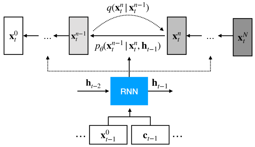
Figure 1: TimeGrad schematic: an RNN conditioned diffusion probabilistic model at some time $t-1$ depicting the fixed forward process that adds Gaussian noise and the learned reverse processes.

3.2 Inference

After training, we wish to predict for each time series in our data set some prediction steps into the future and compare with the corresponding test set time series. As in training, we run the RNN over the last context sized window of the training set to obtain the hidden state $\mathbf{h}_{T}$ via (9). Then we follow the sampling procedure in Algorithm 2 to obtain a sample $\mathbf{x}_{T+1}^{0}$ of the next time step, which we can pass autoregressively to the RNN together with the covariates $\mathbf{c}_{T+1}$ to obtain the next hidden state $\mathbf{h}_{T+1}$ and repeat until the desired forecast horizon has been reached. This process of sampling trajectories from the “warm-up” state $\mathbf{h}_{T}$ can be repeated many times (e.g. $S=100$) to obtain empirical quantiles of the uncertainty of our predictions.

Algorithm 2 Sampling $\mathbf{x}_{t}^{0}$ via annealed Langevin dynamics

  Input: noise $\mathbf{x}_{t}^{N}\sim{\cal{N}}(\mathbf{0},\mathbf{I})$ and state $\mathbf{h}_{t-1}$

  for $n=N$ to $1$ do

     if $n>1$ then

        $\mathbf{z}\sim{\cal{N}}(\mathbf{0},\mathbf{I})$

     else

        $\mathbf{z}=\mathbf{0}$

     end if

     $\mathbf{x}_{t}^{n-1}=\frac{1}{\sqrt{\alpha_{n}}}(\mathbf{x}^{n}_{t}-\frac{\beta_{n}}{\sqrt{1-\bar{\alpha}_{n}}}\mathbf{\epsilon}_{\theta}(\mathbf{x}^{n}_{t},\mathbf{h}_{t-1},n))+\sqrt{\Sigma_{\theta}}\mathbf{z}$

  end for

  Return: $\mathbf{x}_{t}^{0}$

3.3 Scaling

In real-world data, the magnitudes of different time series entities can vary drastically. To normalize scales, we divide each time series entity by their context window mean (or $1$ if it’s zero) before feeding it into the model. At inference, the samples are then multiplied by the same mean values to match the original scale. This rescaling technique simplifies the problem for the model, which is reflected in significantly improved empirical performance as shown in (Salinas et al., 2019b). The other method of a short-cut connection from the input to the output of the function approximator, as done in the multivariate point forecasting method LSTNet (Lai et al., 2018), is not applicable here.

3.4 Covariates

We employ embeddings for categorical features (Charrington, 2018), that allows for relationships within a category, or its context, to be captured when training time series models. Combining these embeddings as features for forecasting yields powerful models like the first place winner of the Kaggle Taxi Trajectory Prediction challenge (De Brébisson et al., 2015). The covariates $\mathbf{c}_{t}$ we use are composed of time-dependent (e.g. day of week, hour of day) and time-independent embeddings, if applicable, as well as lag features depending on the time frequency of the data set we are training on. All covariates are thus known for the periods we wish to forecast.

4 Experiments

We benchmark TimeGrad on six real-world data sets and evaluate against several competitive baselines. The source code of the model will be made available after the review process.

4.1 Evaluation Metric and Data Set

For evaluation, we compute the Continuous Ranked Probability Score (CRPS) (Matheson & Winkler, 1976) on each time series dimension, as well as on the sum of all time series dimensions (the latter denoted by $\mathrm{CRPS}_{\mathrm{sum}}$). CRPS measures the compatibility of a cumulative distribution function $F$ with an observation $x$ as

$$\mathrm{CRPS}(F,x)=\int_{\mathbb{R}}(F(z)-\mathbb{I}\{x\leq z\})^{2}\,\mathrm{d}z,$$

where $\mathbb{I}\{x\leq z\}$ is the indicator function which is one if $x\leq z$ and zero otherwise. CRPS is a proper scoring function, hence CRPS attains its minimum when the predictive distribution $F$ and the data distribution are equal. Employing the empirical CDF of $F$, i.e. $\hat{F}(z)=\frac{1}{S}\sum_{s=1}^{S}\mathbb{I}\{X_{s}\leq z\}$ with $S$ samples $X_{s}\sim F$ as a natural approximation of the predictive CDF, CRPS can be directly computed from simulated samples of the conditional distribution (8) at each time point (Jordan et al., 2019). Finally, $\mathrm{CRPS}_{\mathrm{sum}}$ is obtained by first summing across the $D$ time-series — both for the ground-truth data, and sampled data (yielding $\hat{F}_{\mathrm{sum}}(t)$ for each time point). The results are then averaged over the prediction horizon, i.e. formally $\mathrm{CRPS}_{\mathrm{sum}}=\mathbb{E}_{t}\left[\mathrm{CRPS}\left(\hat{F}_{\mathrm{sum}}(t),\sum_{i}x_{i,t}^{0}\right)\right]$. As proved in (de Bézenac et al., 2020) $\mathrm{CRPS}_{\mathrm{sum}}$ is also a proper scoring function and we use it, instead of likelihood based metrics, since not all methods we compare against yield analytical forecast distributions or likelihoods are not meaningfully defined.

For our experiments we use Exchange (Lai et al., 2018), Solar (Lai et al., 2018), Electricity, Traffic, Taxi and Wikipedia open data sets, preprocessed exactly as in (Salinas et al., 2019a), with their properties listed in Table 1. As can be noted in the table, we do not need to normalize scales for Traffic.

Table 1: Dimension, domain, frequency, total training time steps and prediction length properties of the training data sets used in the experiments.

Data set	Dim. $D$	Dom.	Freq.	Time steps	Pred. steps
Exchange	$8$	$\mathbb{R}^{+}$	day	$6,071$	$30$
Solar	$137$	$\mathbb{R}^{+}$	hour	$7,009$	$24$
Elec.	$370$	$\mathbb{R}^{+}$	hour	$5,833$	$24$
Traffic	$963$	$(0,1)$	hour	$4,001$	$24$
Taxi	$1,214$	$\mathbb{N}$	30-min	$1,488$	$24$
Wiki.	$2,000$	$\mathbb{N}$	day	$792$	$30$

4.2 Model Architecture

We train TimeGrad via SGD using Adam (Kingma & Ba, 2015) with learning rate of $1\text{\times}{10}^{-3}$ on the training split of each data set with $N=100$ diffusion steps using a linear variance schedule starting from $\beta_{1}=$1\text{\times}{10}^{-4}$$ till $\beta_{N}=0.1$. We construct batches of size $64$ by taking random windows (with possible overlaps), with the context size set to the number of prediction steps, from the total time steps of each data set (see Table 1). For testing we use a rolling windows prediction starting from the last context window history before the start of the prediction and compare it to the ground-truth in the test set by sampling $S=100$ trajectories.

The RNN consists of $2$ layers of an LSTM with the hidden state $\mathbf{h}_{t}\in\mathbb{R}^{40}$ and we encode the noise index $n\in\{1,\ldots,N\}$ using the Transformer’s (Vaswani et al., 2017) Fourier positional embeddings, with $N_{\max}=500$, into $\mathbb{R}^{32}$ vectors. The network $\epsilon_{\theta}$ consists of conditional 1-dim dilated ConvNets with residual connections adapted from the WaveNet (van den Oord et al., 2016a) and DiffWave (Kong et al., 2021) models. Figure 2 shows the schematics of a single residual block $i=\{0,\ldots,7\}$ together with the final output from the sum of all the $8$ skip-connections. All, but the last, convolutional network layers have an output channel size of $8$ and we use a bidirectional dilated convolution in each block $i$ by setting its dilation to $2^{i\%2}$. We use a validation set from the training data of the same size as the test set to tune the number of epochs for early stopping.

All experiments run on a single Nvidia V100 GPU with $16$GB of memory.

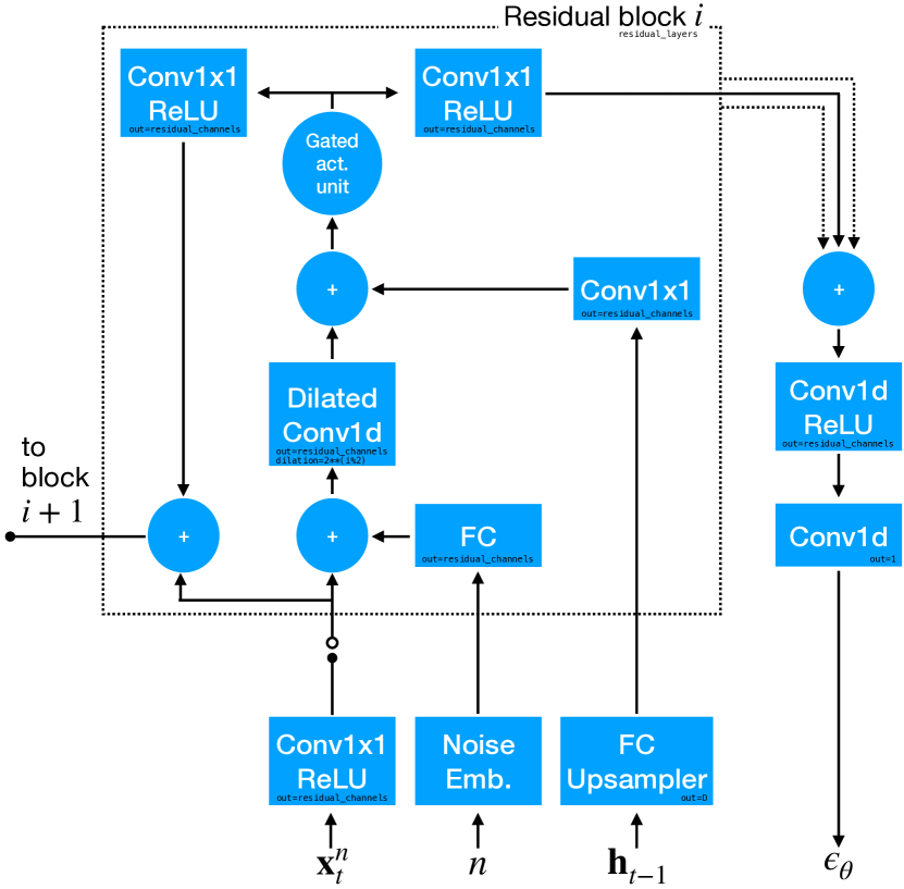
Figure 2: The network architecture of $\epsilon_{\theta}$ consisting of $\mathtt{residual\_layers}=8$ conditional residual blocks with the Gated Activation Unit $\sigma(\cdot)\odot\tanh(\cdot)$ from (van den Oord et al., 2016b); whose skip-connection outputs are summed up to compute the final output. Conv1x1 and Conv1d are 1D convolutional layers with filter size of $1$ and $3$, respectively, circular padding so that the spatial size remains $D$, and all but the last convolutional layer has output channels $\mathtt{residual\_channels}=8$. FC are linear layers used to up/down-sample the input to the appropriate size for broadcasting.

4.3 Results

Table 2: Test set $\mathrm{CRPS}_{\mathrm{sum}}$ comparison (lower is better) of models on six real world data sets. Mean and standard error metrics for TimeGrad obtained by re-training and evaluating $10$ times.

Method	Exchange	Solar	Electricity	Traffic	Taxi	Wikipedia
VES	$\mathbf{0.005}\scriptstyle{\pm 0.000}$	$0.9\scriptstyle{\pm 0.003}$	$0.88\scriptstyle{\pm 0.0035}$	$0.35\scriptstyle{\pm 0.0023}$	-	-
VAR	$\mathbf{0.005}\scriptstyle{\pm 0.000}$	$0.83\scriptstyle{\pm 0.006}$	$0.039\scriptstyle{\pm 0.0005}$	$0.29\scriptstyle{\pm 0.005}$	-	-
VAR-Lasso	$0.012\scriptstyle{\pm 0.0002}$	$0.51\scriptstyle{\pm 0.006}$	$0.025\scriptstyle{\pm 0.0002}$	$0.15\scriptstyle{\pm 0.002}$	-	$3.1\scriptstyle{\pm 0.004}$
GARCH	$0.023\scriptstyle{\pm 0.000}$	$0.88\scriptstyle{\pm 0.002}$	$0.19\scriptstyle{\pm 0.001}$	$0.37\scriptstyle{\pm 0.0016}$	-	-
KVAE	$0.014\scriptstyle{\pm 0.002}$	$0.34\scriptstyle{\pm 0.025}$	$0.051\scriptstyle{\pm 0.019}$	$0.1\scriptstyle{\pm 0.005}$	-	$0.095\scriptstyle{\pm 0.012}$
Vec-LSTM ind-scaling	$0.008\scriptstyle{\pm 0.001}$	$0.391\scriptstyle{\pm 0.017}$	$0.025\scriptstyle{\pm 0.001}$	$0.087\scriptstyle{\pm 0.041}$	$0.506\scriptstyle{\pm 0.005}$	$0.133\scriptstyle{\pm 0.002}$
Vec-LSTM lowrank-Copula	$0.007\scriptstyle{\pm 0.000}$	$0.319\scriptstyle{\pm 0.011}$	$0.064\scriptstyle{\pm 0.008}$	$0.103\scriptstyle{\pm 0.006}$	$0.326\scriptstyle{\pm 0.007}$	$0.241\scriptstyle{\pm 0.033}$
GP scaling	$0.009\scriptstyle{\pm 0.000}$	$0.368\scriptstyle{\pm 0.012}$	$0.022\scriptstyle{\pm 0.000}$	$0.079\scriptstyle{\pm 0.000}$	$0.183\scriptstyle{\pm 0.395}$	$1.483\scriptstyle{\pm 1.034}$
GP Copula	$0.007\scriptstyle{\pm 0.000}$	$0.337\scriptstyle{\pm 0.024}$	$0.0245\scriptstyle{\pm 0.002}$	$0.078\scriptstyle{\pm 0.002}$	$0.208\scriptstyle{\pm 0.183}$	$0.086\scriptstyle{\pm 0.004}$
Transformer MAF	$\mathbf{0.005}\scriptstyle{\pm 0.003}$	$0.301\scriptstyle{\pm 0.014}$	$0.0207\scriptstyle{\pm 0.000}$	$0.056\scriptstyle{\pm 0.001}$	$0.179\scriptstyle{\pm 0.002}$	$0.063\scriptstyle{\pm 0.003}$
TimeGrad	$0.006\scriptstyle{\pm 0.001}$	$\mathbf{0.287}\scriptstyle{\pm 0.02}$	$\mathbf{0.0206}\scriptstyle{\pm 0.001}$	$\mathbf{0.044}\scriptstyle{\pm 0.006}$	$\mathbf{0.114}\scriptstyle{\pm 0.02}$	$\mathbf{0.0485}\scriptstyle{\pm 0.002}$

Using the $\mathrm{CRPS}_{\mathrm{sum}}$ as an evaluation metric, we compare test time predictions of TimeGrad to a wide range of existing methods including classical multivariate methods:

• VAR (Lütkepohl, 2007) a mutlivariate linear vector auto-regressive model with lags corresponding to the periodicity of the data,

• VAR-Lasso a Lasso regularized VAR,

• GARCH (van der Weide, 2002) a multivariate conditional heteroskedastic model and

• VES a innovation state space model (Hyndman et al., 2008);

as well as deep learning based methods namely:

• KVAE (Fraccaro et al., 2017) a variational autoencoder to represent the data on top of a linear state space model which describes the dynamics,

• Vec-LSTM-ind-scaling (Salinas et al., 2019a) which models the dynamics via an RNN and outputs the parameters of an independent Gaussian distribution with mean-scaling,

• Vec-LSTM-lowrank-Copula (Salinas et al., 2019a) which instead parametrizes a low-rank plus diagonal covariance via Copula process,

• GP-scaling (Salinas et al., 2019a) which unrolls an LSTM with scaling on each individual time series before reconstructing the joint distribution via a low-rank Gaussian,

• GP-Copula (Salinas et al., 2019a) which unrolls an LSTM on each individual time series and then the joint emission distribution is given by a low-rank plus diagonal covariance Gaussian copula and

• Transformer-MAF (Rasul et al., 2021) which uses Transformer (Vaswani et al., 2017) to model the temporal conditioning and Masked Autoregressive Flow (Papamakarios et al., 2017) for the distribution emission model.

Table 2 lists the corresponding $\mathrm{CRPS}_{\mathrm{sum}}$ values averaged over $10$ independent runs together with their empirical standard deviations and shows that the TimeGrad model sets the new state-of-the-art on all but the smallest of the benchmark data sets. Note that flow based models must apply continuous transformations onto a continuously connected distribution, making it difficult to model disconnected modes. Flow models assign spurious density to connections between these modes leading to potential inaccuracies. Similarly the generator network in variational autoencoders must learn to map from some continuous space to a possibly disconnected space which might not be possible to learn. In contrast EMBs do not suffer from these issues (Du & Mordatch, 2019).

4.4 Ablation

The length $N$ of the forward process is a crucial hyperparameter, as a bigger $N$ allows the reverse process to be approximately Gaussian (Sohl-Dickstein et al., 2015) which assists the Gaussian parametrization (1) to approximate it better. We evaluate to which extent, if any at all, larger $N$ affects prediction performance, with an ablation study where we record the test set $\mathrm{CRPS}_{\mathrm{sum}}$ of the Electricity data set for different total diffusion process lengths $N=2,4,8,\ldots,256$ while keeping all other hyperparemeters unchanged. The results are then plotted in Figure 3 where we note that $N$ can be reduced down to $\approx 10$ without significant performance loss. An optimal value is achieved at $N\approx 100$ and larger levels are not beneficial if all else is kept fixed.

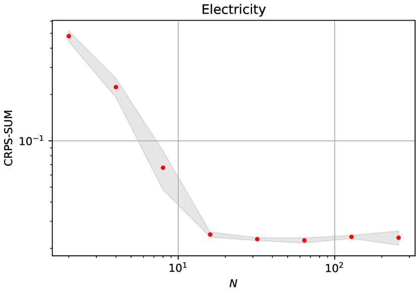
Figure 3: TimeGrad test set $\mathrm{CRPS}_{\mathrm{sum}}$ for Electricity data by varying total diffusion length $N$. Good performance is established already at $N\approx 10$ with optimal value at $N\approx 100$. The mean and standard errors obtained over $5$ independent runs. We see similar behaviour with other data sets.

To highlight the predictions of TimeGrad we show in Figure 4 the predicted median, $50\%$ and $90\%$ distribution intervals of the first $6$ dimensions of the full $963$ dimensional multivariate forecast of the Traffic benchmark.

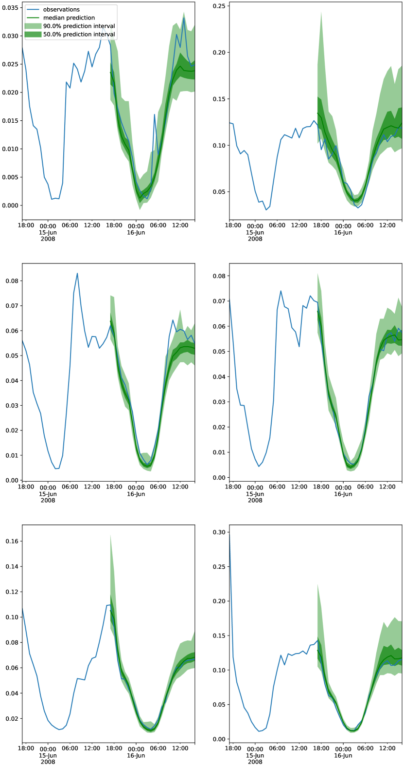
Figure 4: TimeGrad prediction intervals and test set ground-truth for Traffic data of the first $6$ of $963$ dimensions from first rolling-window. Note that neighboring entities have an order of magnitude difference in scales.

5 Related Work

5.1 Energy-Based Methods

The EBM of (Ho et al., 2020) that we adapt is based on methods that learn the gradient of the log-density with respect to the inputs, called Stein Score function (Hyvärinen, 2005; Vincent, 2011), and at inference time use this gradient estimate via Langevin dynamics to sample from the model of this complicated data distribution (Song & Ermon, 2019). These models achieve impressive results for image generation (Ho et al., 2020; Song & Ermon, 2020) when trained in an unsupervised fashion without requiring adversarial optimization. By perturbing the data using multiple noise scales, the learnt Score network captures both coarse and fine-grained data features.

The closest related work to TimeGrad is in the recent non-autoregressive conditional methods for high fidelity waveform generation (Chen et al., 2021; Kong et al., 2021). Although these methods learn the distribution of vector valued data via denoising diffusion methods, as done here, they do not consider its temporal development. Also neighboring dimensions of waveform data are highly correlated and have a uniform scale, which is not necessarily true for multivariate time series problems where neighboring entities occur arbitrarily (but in a fixed order) and can have different scales. (Du & Mordatch, 2019) also use EBMs to model one and multiple steps for a trajectory modeling task in an non-autoregressive fashion.

5.2 Time Series Forecasting

Neural time series methods have recently become popular ways of solving the prediction problem via univariate point forecasting methods (Oreshkin et al., 2020; Smyl, 2020) or univariate probabilistic methods (Salinas et al., 2019b). In the multivariate setting we also have point forecasting methods (Lai et al., 2018; Li et al., 2019) as well as probabilistic methods, like this method, which explicitly model the data distribution using Gaussian copulas (Salinas et al., 2019a), GANs (Yoon et al., 2019), or normalizing flows (de Bézenac et al., 2020; Rasul et al., 2021). Bayesian neural networks can also be used to provide epistemic uncertainty in forecasts as well as detect distributional shifts (Zhu & Laptev, 2018), although these methods often do not perform as well empirically (Wenzel et al., 2020).

6 Conclusion and Future Work

We have presented TimeGrad, a versatile multivariate probabilistic time series forecasting method that leverages the exceptional performance of EBMs to learn and sample from the distribution of the next time step, autoregressivly. Analysis of TimeGrad on six commonly used time series benchmarks establishes the new state-of-the-art against competitive methods.

We note that while training TimeGrad we do not need to loop over the EBM function approximator $\epsilon_{\theta}$, unlike in the normalizing flow setting where we have multiple stacks of bijections. However while sampling we do loop $N$ times over $\epsilon_{\theta}$. A possible strategy to improve sampling times introduced in (Chen et al., 2021) uses a combination of improved variance schedule and an $L_{1}$ loss to allow sampling with fewer steps at the cost of a small reduction in quality if such a trade-off is required. A recent paper (Song et al., 2021) generalize the diffusion processes via a class of non-Markovian processes which also allows for faster sampling.

The use of normalizing flows for discrete valued data dictates that one dequantizes it (Theis et al., 2016), by adding uniform noise to the data, before using the flows to learn. Dequantization is not needed in the EBM setting and future work could explore methods of explicitly modeling discrete distributions.

As noted in (Du & Mordatch, 2019) EBMs exhibit better out-of-distribution (OOD) detection than other likelihood models. Such a task requires models to have a high likelihood on the data manifold and low at all other locations. Surprisingly (Nalisnick et al., 2019) showed that likelihood models, including flows, were assigning higher likelihoods to OOD data whereas EBMs do not suffer from this issue since they penalize high probability under the model but low probability under the data distribution explicitly. Future work could evaluate the usage of TimeGrad for anomaly detection tasks.

For long time sequences, one could replace the RNN with a Transformer architecture (Rasul et al., 2021) to provide better conditioning for the EBM emission head. Concurrently, since EBMs are not constrained by the form of their functional approximators, one natural way to improve the model would be to incorporate architectural choices that best encode the inductive bias of the problem being tackled, for example with graph neural networks (Niu et al., 2020) when the relationships between entities are known.

References

- Benidis et al. (2020) Benidis, K., Rangapuram, S. S., Flunkert, V., Wang, B., Maddix, D., Turkmen, C., Gasthaus, J., Bohlke-Schneider, M., Salinas, D., Stella, L., Callot, L., and Januschowski, T. Neural forecasting: Introduction and literature overview, 2020.
- Charrington (2018) Charrington, S. TWiML & AI Podcast: Systems and Software for Machine Learning at Scale with Jeff Dean, 2018. URL https://bit.ly/2G0LmGg.
- Chen et al. (2021) Chen, N., Zhang, Y., Zen, H., Weiss, R. J., Norouzi, M., and Chan, W. WaveGrad: Estimating gradients for waveform generation. In International Conference on Learning Representations 2021 (Conference Track), 2021. URL https://openreview.net/forum?id=NsMLjcFaO8O.
- Chung et al. (2014) Chung, J., Gulcehre, C., Cho, K., and Bengio, Y. Empirical evaluation of gated recurrent neural networks on sequence modeling. In NIPS 2014 Workshop on Deep Learning, December 2014, 2014.
- de Bézenac et al. (2020) de Bézenac, E., Rangapuram, S. S., Benidis, K., Bohlke-Schneider, M., Kurle, R., Stella, L., Hasson, H., Gallinari, P., and Januschowski, T. Normalizing Kalman Filters for Multivariate Time series Analysis. In Advances in Neural Information Processing Systems, volume 33. Curran Associates, Inc., 2020.
- De Brébisson et al. (2015) De Brébisson, A., Simon, E., Auvolat, A., Vincent, P., and Bengio, Y. Artificial Neural Networks Applied to Taxi Destination Prediction. In Proceedings of the 2015th International Conference on ECML PKDD Discovery Challenge - Volume 1526, ECMLPKDDDC’15, pp. 40–51, Aachen, Germany, Germany, 2015. CEUR-WS.org. URL http://dl.acm.org/citation.cfm?id=3056172.3056178.
- Dinh et al. (2017) Dinh, L., Sohl-Dickstein, J., and Bengio, S. Density estimation using Real NVP. In 5th International Conference on Learning Representations, ICLR 2017, Toulon, France, April 24-26, 2017, Conference Track Proceedings. OpenReview.net, 2017. URL https://openreview.net/forum?id=HkpbnH9lx.
- Du & Mordatch (2019) Du, Y. and Mordatch, I. Implicit Generation and Modeling with Energy Based Models. In Wallach, H., Larochelle, H., Beygelzimer, A., d'Alché-Buc, F., Fox, E., and Garnett, R. (eds.), Advances in Neural Information Processing Systems, volume 32, pp. 3608–3618. Curran Associates, Inc., 2019. URL https://proceedings.neurips.cc/paper/2019/file/378a063b8fdb1db941e34f4bde584c7d-Paper.pdf.
- Fraccaro et al. (2017) Fraccaro, M., Kamronn, S., Paquet, U., and Winther, O. A Disentangled Recognition and Nonlinear Dynamics Model for Unsupervised Learning. In Guyon, I., Luxburg, U. V., Bengio, S., Wallach, H., Fergus, R., Vishwanathan, S., and Garnett, R. (eds.), Advances in Neural Information Processing Systems, volume 30, pp. 3601–3610. Curran Associates, Inc., 2017. URL https://proceedings.neurips.cc/paper/2017/file/7b7a53e239400a13bd6be6c91c4f6c4e-Paper.pdf.
- Graves (2013) Graves, A. Generating Sequences With Recurrent Neural Networks. arXiv preprint arXiv:1308.0850, 2013.
- Hinton (2002) Hinton, G. E. Training Products of Experts by Minimizing Contrastive Divergence. Neural Computation, 14(8):1771––1800, August 2002. ISSN 0899-7667. doi: 10.1162/089976602760128018. URL https://doi.org/10.1162/089976602760128018.
- Ho et al. (2020) Ho, J., Jain, A., and Abbeel, P. Denoising Diffusion Probabilistic Models. In Wallach, H., Larochelle, H., Beygelzimer, A., d'Alché-Buc, F., Fox, E., and Garnett, R. (eds.), Advances in Neural Information Processing Systems, volume 33. Curran Associates, Inc., 2020. URL https://papers.nips.cc/paper/2020/file/4c5bcfec8584af0d967f1ab10179ca4b-Paper.pdf.
- Hochreiter & Schmidhuber (1997) Hochreiter, S. and Schmidhuber, J. Long Short-Term Memory. Neural Computation, 9(8):1735–1780, November 1997. ISSN 0899-7667. doi: 10.1162/neco.1997.9.8.1735.
- Hyndman & Athanasopoulos (2018) Hyndman, R. and Athanasopoulos, G. Forecasting: Principles and practice. OTexts, 2018. ISBN 9780987507112.
- Hyndman et al. (2008) Hyndman, R., Koehler, A., Ord, K., and Snyder, R. Forecasting with exponential smoothing. The state space approach, chapter 17, pp. 287–300. Springer-Verlag, 2008. doi: 10.1007/978-3-540-71918-2.
- Hyvärinen (2005) Hyvärinen, A. Estimation of Non-Normalized Statistical Models by Score Matching. Journal of Machine Learning Research, 6(24):695–709, 2005. URL http://jmlr.org/papers/v6/hyvarinen05a.html.
- Jordan et al. (2019) Jordan, A., Krüger, F., and Lerch, S. Evaluating Probabilistic Forecasts with scoringRules. Journal of Statistical Software, Articles, 90(12):1–37, 2019. ISSN 1548-7660. doi: 10.18637/jss.v090.i12. URL https://www.jstatsoft.org/v090/i12.
- Kingma & Ba (2015) Kingma, D. P. and Ba, J. Adam: A method for stochastic optimization. In International Conference on Learning Representations (ICLR), 2015.
- Kingma & Welling (2019) Kingma, D. P. and Welling, M. An Introduction to Variational Autoencoders. Foundations and Trends in Machine Learning, 12(4):307–392, 2019. doi: 10.1561/2200000056. URL https://doi.org/10.1561/2200000056.
- Kong et al. (2021) Kong, Z., Ping, W., Huang, J., Zhao, K., and Catanzaro, B. DiffWave: A Versatile Diffusion Model for Audio Synthesis. In International Conference on Learning Representations 2021 (Conference Track), 2021. URL https://openreview.net/forum?id=a-xFK8Ymz5J.
- Lai et al. (2018) Lai, G., Chang, W.-C., Yang, Y., and Liu, H. Modeling Long- and Short-Term Temporal Patterns with Deep Neural Networks. In The 41st International ACM SIGIR Conference on Research & Development in Information Retrieval, SIGIR ’18, pp. 95–104, New York, NY, USA, 2018. ACM. ISBN 978-1-4503-5657-2. doi: 10.1145/3209978.3210006. URL http://doi.acm.org/10.1145/3209978.3210006.
- LeCun et al. (2006) LeCun, Y., Chopra, S., Hadsell, R., Ranzato, M., and Huang, F. A Tutorial on Energy-Based Learning. In Bakir, G., Hofman, T., Schölkopf, B., Smola, A., and Taskar, B. (eds.), Predicting Structured Data. MIT Press, 2006.
- Li et al. (2019) Li, S., Jin, X., Xuan, Y., Zhou, X., Chen, W., Wang, Y.-X., and Yan, X. Enhancing the locality and breaking the memory bottleneck of transformer on time series forecasting. In Wallach, H., Larochelle, H., Beygelzimer, A., d’Alché Buc, F., Fox, E., and Garnett, R. (eds.), Advances in Neural Information Processing Systems 32, pp. 5244–5254. Curran Associates, Inc., 2019.
- Lütkepohl (2007) Lütkepohl, H. New Introduction to Multiple Time Series Analysis. Springer Berlin Heidelberg, 2007. ISBN 9783540262398. URL https://books.google.de/books?id=muorJ6FHIiEC.
- Matheson & Winkler (1976) Matheson, J. E. and Winkler, R. L. Scoring Rules for Continuous Probability Distributions. Management Science, 22(10):1087–1096, 1976.
- Nalisnick et al. (2019) Nalisnick, E., Matsukawa, A., Teh, Y. W., Gorur, D., and Lakshminarayanan, B. Do Deep Generative Models Know What They Don’t Know? In International Conference on Learning Representations, 2019. URL https://openreview.net/forum?id=H1xwNhCcYm.
- Niu et al. (2020) Niu, C., Song, Y., Song, J., Zhao, S., Grover, A., and Ermon, S. Permutation Invariant Graph Generation via Score-Based Generative Modeling. In Chiappa, S. and Calandra, R. (eds.), The 23rd International Conference on Artificial Intelligence and Statistics, AISTATS 2020, 26-28 August 2020, Online [Palermo, Sicily, Italy], volume 108 of Proceedings of Machine Learning Research, pp. 4474–4484. PMLR, 2020.
- Oreshkin et al. (2020) Oreshkin, B. N., Carpov, D., Chapados, N., and Bengio, Y. N-BEATS: Neural basis expansion analysis for interpretable time series forecasting. In International Conference on Learning Representations, 2020. URL https://openreview.net/forum?id=r1ecqn4YwB.
- Papamakarios et al. (2017) Papamakarios, G., Pavlakou, T., and Murray, I. Masked Autoregressive Flow for Density Estimation. Advances in Neural Information Processing Systems 30, 2017.
- Papamakarios et al. (2019) Papamakarios, G., Nalisnick, E., Rezende, D. J., Mohamed, S., and Lakshminarayanan, B. Normalizing Flows for Probabilistic Modeling and Inference, 2019.
- Rasul et al. (2021) Rasul, K., Sheikh, A.-S., Schuster, I., Bergmann, U., and Vollgraf, R. Multivariate Probabilistic Time Series Forecasting via Conditioned Normalizing Flows. In International Conference on Learning Representations 2021 (Conference Track), 2021. URL https://openreview.net/forum?id=WiGQBFuVRv.
- Salinas et al. (2019a) Salinas, D., Bohlke-Schneider, M., Callot, L., Medico, R., and Gasthaus, J. High-dimensional multivariate forecasting with low-rank Gaussian Copula Processes. In Wallach, H., Larochelle, H., Beygelzimer, A., d’Alché Buc, F., Fox, E., and Garnett, R. (eds.), Advances in Neural Information Processing Systems 32, pp. 6824–6834. Curran Associates, Inc., 2019a.
- Salinas et al. (2019b) Salinas, D., Flunkert, V., Gasthaus, J., and Januschowski, T. DeepAR: Probabilistic forecasting with autoregressive recurrent networks. International Journal of Forecasting, 2019b. ISSN 0169-2070. URL http://www.sciencedirect.com/science/article/pii/S0169207019301888.
- Smyl (2020) Smyl, S. A hybrid method of exponential smoothing and recurrent neural networks for time series forecasting. International Journal of Forecasting, 36(1):75–85, 2020. ISSN 0169-2070. doi: https://doi.org/10.1016/j.ijforecast.2019.03.017. URL http://www.sciencedirect.com/science/article/pii/S0169207019301153. M4 Competition.
- Sohl-Dickstein et al. (2015) Sohl-Dickstein, J., Weiss, E., Maheswaranathan, N., and Ganguli, S. Deep Unsupervised Learning using Nonequilibrium Thermodynamics. In Bach, F. and Blei, D. (eds.), Proceedings of the 32nd International Conference on Machine Learning, volume 37 of Proceedings of Machine Learning Research, pp. 2256–2265, Lille, France, 2015. PMLR. URL http://proceedings.mlr.press/v37/sohl-dickstein15.html.
- Song et al. (2021) Song, J., Meng, C., and Ermon, S. Denoising Diffusion Implicit Models. In International Conference on Learning Representations 2021 (Conference Track), 2021. URL https://openreview.net/pdf?id=St1giarCHLP.
- Song & Ermon (2019) Song, Y. and Ermon, S. Generative Modeling by Estimating Gradients of the Data Distribution. In Wallach, H., Larochelle, H., Beygelzimer, A., d'Alché-Buc, F., Fox, E., and Garnett, R. (eds.), Advances in Neural Information Processing Systems, volume 32, pp. 11918–11930. Curran Associates, Inc., 2019. URL https://proceedings.neurips.cc/paper/2019/file/3001ef257407d5a371a96dcd947c7d93-Paper.pdf.
- Song & Ermon (2020) Song, Y. and Ermon, S. Improved Techniques for Training Score-Based Generative Models. In Wallach, H., Larochelle, H., Beygelzimer, A., d'Alché-Buc, F., Fox, E., and Garnett, R. (eds.), Advances in Neural Information Processing Systems, volume 33. Curran Associates, Inc., 2020. URL https://proceedings.neurips.cc/paper/2020/file/92c3b916311a5517d9290576e3ea37ad-Paper.pdf.
- Song & Kingma (2021) Song, Y. and Kingma, D. P. How to Train Your Energy-Based Models. 2021. URL https://arxiv.org/abs/2101.03288.
- Sutskever et al. (2014) Sutskever, I., Vinyals, O., and Le, Q. V. Sequence to Sequence Learning with Neural Networks. In Ghahramani, Z., Welling, M., Cortes, C., Lawrence, N., and Weinberger, K. (eds.), Advances in Neural Information Processing Systems 27, pp. 3104–3112. Curran Associates, Inc., 2014.
- Theis et al. (2016) Theis, L., van den Oord, A., and Bethge, M. A note on the evaluation of generative models. In International Conference on Learning Representations, 2016. URL http://arxiv.org/abs/1511.01844. arXiv:1511.01844.
- Tsay (2014) Tsay, R. S. Multivariate Time Series Analysis: With R and Financial Applications. Wiley Series in Probability and Statistics. Wiley, 2014. ISBN 9781118617908.
- van den Oord et al. (2016a) van den Oord, A., Dieleman, S., Zen, H., Simonyan, K., Vinyals, O., Graves, A., Kalchbrenner, N., Senior, A., and Kavukcuoglu, K. WaveNet: A Generative Model for Raw Audio. In The 9th ISCA Speech Synthesis Workshop, Sunnyvale, CA, USA, 13-15 September 2016, pp. 125. ISCA, 2016a. URL http://www.isca-speech.org/archive/SSW_2016/abstracts/ssw9_DS-4_van_den_Oord.html.
- van den Oord et al. (2016b) van den Oord, A., Kalchbrenner, N., Espeholt, L., kavukcuoglu, k., Vinyals, O., and Graves, A. Conditional Image Generation with PixelCNN Decoders. In Lee, D., Sugiyama, M., Luxburg, U., Guyon, I., and Garnett, R. (eds.), Advances in Neural Information Processing Systems, volume 29, pp. 4790–4798. Curran Associates, Inc., 2016b. URL https://proceedings.neurips.cc/paper/2016/file/b1301141feffabac455e1f90a7de2054-Paper.pdf.
- van den Oord et al. (2016c) van den Oord, A., Kalchbrenner, N., and Kavukcuoglu, K. Pixel Recurrent Neural Networks. In Balcan, M. F. and Weinberger, K. Q. (eds.), Proceedings of The 33rd International Conference on Machine Learning, volume 48 of Proceedings of Machine Learning Research, pp. 1747–1756, New York, New York, USA, 20–22 Jun 2016c. PMLR. URL http://proceedings.mlr.press/v48/oord16.html.
- van der Weide (2002) van der Weide, R. GO-GARCH: a multivariate generalized orthogonal GARCH model. Journal of Applied Econometrics, 17(5):549–564, 2002. doi: 10.1002/jae.688.
- Vaswani et al. (2017) Vaswani, A., Shazeer, N., Parmar, N., Uszkoreit, J., Jones, L., Gomez, A. N., Kaiser, L. u., and Polosukhin, I. Attention is All you Need. In Guyon, I., Luxburg, U., Bengio, S., Wallach, H., Fergus, R., Vishwanathan, S., and Garnett, R. (eds.), Advances in Neural Information Processing Systems 30, pp. 5998–6008. Curran Associates, Inc., 2017. URL http://papers.nips.cc/paper/7181-attention-is-all-you-need.pdf.
- Vincent (2011) Vincent, P. A Connection Between Score Matching and Denoising Autoencoders. Neural Computation, 23(7):1661–1674, 2011. URL https://doi.org/10.1162/NECO_a_00142.
- Wenzel et al. (2020) Wenzel, F., Roth, K., Veeling, B., Swiatkowski, J., Tran, L., Mandt, S., Snoek, J., Salimans, T., Jenatton, R., and Nowozin, S. How good is the Bayes posterior in deep neural networks really? In III, H. D. and Singh, A. (eds.), Proceedings of the 37th International Conference on Machine Learning, volume 119 of Proceedings of Machine Learning Research, pp. 10248–10259. PMLR, 13–18 Jul 2020. URL http://proceedings.mlr.press/v119/wenzel20a.html.
- Yoon et al. (2019) Yoon, J., Jarrett, D., and van der Schaar, M. Time-series Generative Adversarial Networks. In Wallach, H., Larochelle, H., Beygelzimer, A., d'Alché-Buc, F., Fox, E., and Garnett, R. (eds.), Advances in Neural Information Processing Systems, volume 32, pp. 5508–5518. Curran Associates, Inc., 2019. URL https://proceedings.neurips.cc/paper/2019/file/c9efe5f26cd17ba6216bbe2a7d26d490-Paper.pdf.
- Zhu & Laptev (2018) Zhu, L. and Laptev, N. Deep and Confident Prediction for Time Series at Uber. In 2017 IEEE International Conference on Data Mining Workshops (ICDMW), volume 00, pp. 103–110, November 2018. doi: 10.1109/ICDMW.2017.19. URL doi.ieeecomputersociety.org/10.1109/ICDMW.2017.19.