On McMullen’s algorithm for the Hausdorff dimension of Complex Schottky Groups

Abstract.

We provide a generalization of the McMullen’s algorithm to approximate the Hausdorff dimension of the limit set for convex-cocompact subgroups of isometries of the Complex Hyperbolic Plane.

Introduction

The Hausdorff dimension is a bi-Lipschitz invariant, and in the case of the Kleinian groups allows us to understand what kind of fractal spaces can be a limit set of Kleinian groups. In 1998, McMullen ([16]) proposed an algorithm to approximates the Hausdorff dimension of a set associated with a conformal dynamical system (as Julia sets or limit set of a geometrically finite Kleinian groups). Naively, McMullen’s algorithm works as follows:

1. For a Markov partition of the dynamical system. We compute the transition matrix T using the data of the dynamical system.

2. We solve for $\alpha$ such that the spectral radius of $T^{\alpha}$ is 1. The matrix $T^{\alpha}$ is equal to the matrix where each entry is the entry of T powered by $\alpha.$ The power $\alpha$ is an approximation of the dimension of the conformal measure.

3. We refine the Markov partition and do step 1 again.

For geometrically finite Kleinian groups, the conformal dynamical system conformed by the group and the associated Patterson-Sullivan measure (see [20],[23]). The dimension of the associated Patterson-Sullivan measures coincides with the Hausdorff dimension of its limit set; from the previous, McMullen’s algorithm works to approximate the Hausdorff dimension of the Kleinian group limit set.

The Patterson-Sullivan theorems are not exclusive of the real hyperbolic geometry. Indeed this construction is generalized to different scenarios and geometries (see [1], [8], [9], [21]), and all of them relates to the hyperbolic properties of the space. In particular, the Patterson-Sullivan theory is valid for the complex hyperbolic plane $\mathbb{H}^{2}_{\mathbb{C}}$ and subgroups of $Isom(\mathbb{H}^{2}_{\mathbb{C}}).$

In the complex hyperbolic setting, the discrete subgroups of $\mbox{{Isom}}(\mathbb{H}^{2}_{\mathbb{C}})$ are a particular case of complex Kleinian groups, a term introduced by Seade and Verjovsky (see [6]) as a generalization of the classic Kleinian group but for actions of $PSL(n+1,\mathbb{C})$ in the complex projective n-space. The conformal dimension associated with a convex-cocompact subgroup of $\mbox{{Isom}}(\mathbb{H}^{2}_{\mathbb{C}})$ also satisfies that its dimension coincides with the Hausdorff dimension of the limit set of the group in $\partial\mathbb{H}^{2}_{\mathbb{C}}.$

In the present, we propose a generalization of the McMullen algorithm. The algorithm we propose allows us to approximate the Hausdorff dimension of the limit set of a convex-cocompact discrete subgroup of $\mbox{{Isom}}(\mathbb{H}^{2}_{\mathbb{C}}),$ see, Theorems 3.4, 3.3 and 3.4. Also, we provide a pseudo-code for its computational implementation, see Appendix. We have to mention that the generalization doesn’t follow directly from McMullen’s paper. In the complex hyperbolic setting, the Patterson-Sullivan measure is defined using the visual metrics in $\partial\mathbb{H}^{2}_{\mathbb{C}},$ meanwhile the Markov partition in Theorem 3.1 is defined using the Cygan metric in $\partial\mathbb{H}^{2}_{\mathbb{C}}\setminus\{\infty\},$ this Markov partition definition follow the same spirit as the one in McMullen’s work. Due to the work of Paulin-Hersonsky ([15]), we obtain Theorem 3.3 that implies that there exists a Markov partition for the boundary using the visual metric with the same properties of the one using the Cygan metric.

Theorem 3.4, states the order of the approximation of the generalized algorithm coincides with the one proposed by McMullen.

The paper is organized as follows: Section 1 we settle the notation and construction that we will use in subsequent sections. Section 2 deals with the construction of Schottky groups as subgroups of $\mbox{{Isom}}(\mathbb{H}^{2}_{\mathbb{C}})$ generated by complex inversions, and we prove some general facts about them. Finally, in Section 3 we construct the Markov partition associated with a Schottky group, we state the McMullen algorithm and some examples.

1. Preliminaries

1.1. Complex Hyperbolic Plane

Let $\mathbb{C}^{2,1}$ denote the vector space $\mathbb{C}^{3}$ with the Hermitian form

(1) $$\left\langle\left(\!\begin{array}[]{c}z_{1}\\ z_{2}\\ 1\end{array}\!\right)\left(\!\begin{array}[]{c}w_{1}\\ w_{2}\\ 1\end{array}\!\right)\right\rangle=\overline{z}_{1}w_{3}+\overline{z}_{2}w_{2}+\overline{z}_{3}w_{1}.$$

and let $\pi:\mathbb{C}^{3}\setminus\{0\}\rightarrow\mathbb{P}^{2}_{\mathbb{C}}$ the natural projection. The complex hyperbolic plane, denoted by $\mathbb{H}^{2}_{\mathbb{C}},$ is the image under $\pi$ of the set of negative vectors in $\mathbb{C}^{2,1}.$ The boundary of $\mathbb{H}^{2}_{\mathbb{C}}$ is defined as the image under $\pi$ of the set of null vectors and we will denoted by $\partial\mathbb{H}^{2}_{\mathbb{C}}.$ The complex hyperbolic plane equipped with the Bergman metric (see [13]) is a complete Kähler manifold of constant holomorphic sectional curvature -1.

Let $U(2,1)$ denote the unitary group associated to the Hermitian form 1. The set of holomorphic isometries of $\mathbb{H}^{2}_{\mathbb{C}}$ is the projective unitary group $PU(2,1)$ and the full group of isometries $\mbox{Iso}(\mathbb{H}^{2}_{\mathbb{C}})$ is generated by $PU(2,1)$ and the complex conjugation (see [13], [19]).

1.1.1. Horospherical coordinates and Heisenberg structure.

Let $z\in\partial\mathbb{H}^{2}_{\mathbb{C}},$ given by

$$z=\left[\begin{array}[]{c}z_{1}\\ z_{2}\\ 1\end{array}\right],$$

then $z$ has to satisfy $2\Re(z_{1})+|z_{2}|^{2}=0.$ So writing $z_{2}=\sqrt{2}\zeta$ and $z_{1}=-|\zeta|^{2}+iv,$ we ensure that the previous equation is satisfied and we obtain an identification of $\partial\mathbb{H}^{2}_{\mathbb{C}}$ with the one point compactification of $\mathbb{C}\times\mathbb{R}.$ The boundary has a structure of Heisenberg group (see [13],[19]) with group operation

$$(\zeta,v)\ast(\xi,t)=(\zeta+\xi,v+t+2\Im(\overline{\zeta}\xi))$$

we will denote by $\mathfrak{H}$ the set $\mathbb{C}\times\mathbb{R}$ with the Heisenberg structure.

For a fixed $u\in\mathbb{R}_{+},$ and consider the points $z\in\mathbb{H}^{2}_{\mathbb{C}}$ such that $\langle z,z\rangle=-2u,$ these points have the form

(2) $$\left[\begin{array}[]{c}-|\zeta|^{2}-u+iv\\ \sqrt{2}\zeta\\ 1\end{array}\right],$$

so a point $z$ correspond to a triplet $(\zeta,v,u)\in\mathfrak{H}\times\mathbb{R}_{+},$ known as horospherical coordinates. Let us denote by $H_{u}$ the locus of points in $\mathbb{H}^{2}_{\mathbb{C}}$ such that $\langle z,z\rangle=-2u,$ this set is called horosphere of weight $u$, $H_{u}$ carries the Heisenberg group structure. It will be useful to identify the finite points of $\partial\mathbb{H}^{2}_{\mathbb{C}}\setminus\{\infty\}$ with $H_{0}.$ We will define the horoball of weight u as the union of the $H_{t}$ for $t\geq u,$ so the horoball of weight zero is equal to $\mathbb{H}^{2}_{\mathbb{C}}.$

The Heisenberg norm is given by $|(\zeta,v)|_{0}=\left||\zeta|^{2}+iv|\right|^{\frac{1}{2}},$ this norm induces a metric on $\mathfrak{H},$ called the Cygan metric, defined by

(3) $$d_{Cyg}((\zeta_{1},v_{1}),(\zeta_{2},v_{2}))=|(\zeta_{1}-\zeta_{2},-v_{1}-+v_{2}-2\Im(\overline{\zeta}_{2}\zeta_{1}))|_{0}.$$

The previous metric can be extended to the whole $\overline{\mathbb{H}^{2}_{\mathbb{C}}}\setminus\{\infty\}$ as an incomplete metric as follows

$$d_{Cyg}((\zeta_{1},u_{1},v_{1}),(\zeta_{2},u_{2},v_{2}))=||\zeta_{1}-\zeta_{2}|^{2}+|u_{1}-u_{2}|+i(-v_{1}+v_{2}-2\Im(\overline{\zeta}_{2}\zeta_{1}))|^{\frac{1}{2}}.$$

We will denote the Cygan balls by $B((\xi,t),r)$ at the set of points $(\zeta,v,u)\in\mathfrak{H}\times\mathbb{R}_{+}$ such that $d_{Cyg}((\xi,t,0),(\zeta,v,u))=r,$ and we will call Cygan sphere, $S((\xi,t),r),$ at the intersection $B((\xi,t),r)\cap\partial\mathbb{H}^{2}_{\mathbb{C}}.$

The Heisenberg group acts on itself by

• Heisenberg translations: $T_{(\zeta,v)}(\xi,t)=(\zeta+\xi,v+t+2\Im(\overline{\zeta}\xi)).$

• Complex dilatations: $d_{\lambda}(\zeta,v)=(\lambda z,|\lambda|^{2}v).$

The first ones are isometries of the Cygan metric, and for the complex dilations these are isometries if and only if $|\lambda|=1.$

We will call an embedded copy of $\mathbb{H}^{1}_{\mathbb{C}}$ on $\mathbb{H}^{2}_{\mathbb{C}}$ a complex geodesic, which is a totally geodesic submanifold of dimension 2 and constant sectional curvature equal -1. The intersection of a complex geodesic $L$ with $\partial\mathbb{H}^{2}_{\mathbb{C}}$ is called chain and denoted by $\partial L.$ Chains passing through $\infty$ are called vertical or infinite chains and otherwise is called finite chain. For every finite chain $C,$ there exist a translation and a complex dilatation such that $C$ is image of $\mathbb{S}^{1}\times\{0\}\subset\mathfrak{H}$ under these mappings. For every complex geodesic $L,$ there is a unique element of $PU(2,1)$ whose fixed-point set is $L,$ these maps are called complex reflections. The action of a complex reflection on the boundary preserves the chain associated to the complex geodesic.

The following lemma gives a description of the Cygan metric by the action of an element of $PU(2,1).$

Lemma 1.1.

Let $g\in PU(2,1)$ that does not fix $\infty.$ Then there exists a positive number $r_{g}$ depending only in $g$ such that for all $z,w\in\partial\mathbb{H}^{2}_{\mathbb{C}}\setminus\{\infty,g^{-1}(\infty)\},$ we have:

1. $d_{Cyg}(g(z),g(w))=\frac{r^{2}_{g}d_{Cyg}(z,w)}{d_{Cyg}(z,g^{-1}(\infty))d_{Cyg}(w,g^{-1}(\infty))},$

2. $d_{Cyg}(g(z),g(\infty))=\frac{r^{2}_{g}}{d_{Cyg}(z,g^{-1}(\infty))}.$

An important consequence of the previous lemma is that $g$ sends the Cygan sphere of radius $r_{g}$ and centre $g^{-1}(\infty)$ to the Cygan sphere of radius $r_{g}$ and center $g(\infty).$ So as an analogous of real hyperbolic geometry, it’s defined the isometric sphere of $g$ as the Cygan sphere of radius $r_{g}$ and center $g^{-1}(\infty).$

Proposition 1.2 ([18]).

Let $h$ be an element of $PU(2,1)$ not fixing $\infty.$ Then the Cygan sphere of radius $r$ and centre $h^{-1}(\infty)$ is mapped by $h$ into the Cygan sphere of radius $r^{2}_{h}/r$ and centered at $h(\infty).$

1.2. Patterson-Sullivan Measures for subgroups of $PU(2,1)$

A discrete subgroup $\Gamma$ of $PU(2,1)$ is called a complex Kleinian group (see [6]), these groups gives a partition of $\overline{\mathbb{H}^{2}_{\mathbb{C}}}$ in two invariant sets:

• The first is the Chen-Greenberg limit set who is the closure of the cluster points of $\Gamma$ orbits of points in $\mathbb{H}^{2}_{\mathbb{C}},$ is a subset of $\partial\mathbb{H}^{2}_{\mathbb{C}}$ and it is denoted by $\Lambda_{CG}(\Gamma).$

• The second is the discontinuity region, denoted by $\Omega(\Gamma),$ given by $\overline{\mathbb{H}^{2}_{\mathbb{C}}}\setminus\Lambda_{CG}(\Gamma).$

In the classical setting, for a convex-cocompact subgroup $\Gamma$ of $PSL(2,\mathbb{C}),$ there is a density $\mu$ associated to $\Gamma,$ such that it is invariant by the group (see [24]). The existence of this density is not exclusively for $\mathbb{H}^{3}$ and convex cocompact subgroups of $PSL(2,C).$ This theory can be extended for hyperbolic manifolds or non-postively curved spaces ([9],[21],[3]).

Definition 1.3.

Let $X$ be a complete simply connected Riemannian manifold with non-positive curvature and $\Gamma$ a discrete subgroup of $Isom(X),$ a map $x\mapsto\nu_{x}$ from $X$ to the set of Radom measures on $\partial X$ wich:

1. It is $\Gamma-$equivariant.

2. If $x,y\in X,$ then $\nu_{x}$ and $\nu_{y}$ are equivalent.

3. For every $\zeta\in\partial X,$ we have

   $$\frac{d\nu_{y}}{d\nu_{x}}(\zeta)=e^{-\beta b_{\zeta}(y,x)},$$

   where $b_{\zeta}(y,x)$ is the Busemann function.

We will say that this map is a $\Gamma-$conformal density of dimension $\beta.$

Theorem 1.4 ([9]).

Let $(X,d)$ a proper hyperbolic space and $\Gamma$ a group acting on $X$ by isometries properly discontinuous and convex-cocompactly. Let $d_{a}$ the visual metric on $\partial X$ and $\Lambda(\Gamma)$ the limit set of $\Gamma.$ Put $D=\delta_{a}(\Gamma)$ the exponent of growth of $\Gamma$ and $H=H^{D}$ the $D-$Hausdorff measure on $\Lambda(\Gamma)$ with respect to $d_{a}.$ Then

1. $\delta_{a}(\Gamma)$ is the Hausdorff dimension of $\Lambda(\Gamma).$

2. $H$ on $\Lambda(\Gamma)$ is a $\Gamma-$conformal density of dimension $\delta_{a}(\Gamma).$

3. If $\mu$ is a $\Gamma-$conformal measure of dimension $D^{\prime}$ with support $\Lambda(\Gamma)$ then $D^{\prime}=D=\delta_{a}(\Gamma)$ and $\mu$ and $H$ are equivariant.

For discrete subgroups of $PU(2,1),$ the convex cocompact groups are characterized by the type of its limit point.

Definition 1.5.

A sequence $(x_{i})_{i\in\mathbb{N}}$ of different points in $\mathbb{H}^{2}_{\mathbb{C}}$ is said to converge to a point $\zeta\in\partial\mathbb{H}^{2}_{\mathbb{C}}$ conically if there exists a geodesic ray $x\zeta$ in $\mathbb{H}^{2}_{\mathbb{C}}$ and a constant $R<\infty$ such that:

$$d(x_{i},x\zeta)\leq R$$

for all $i$ and $\displaystyle{\lim_{i\to\infty}}x_{i}=\zeta.$ We will denote $\Lambda^{c}_{\Gamma}$ the set of conical limit points.

Theorem 1.6 ([4]).

A discrete group $G<PU(2,1)$ is convex-cocompact if and only if every limit point of $\Gamma$ is conical.

1.3. Anosov Representations into $PU(2,1)$.

Let $G$ be a semi-simple Lie group with finite center and Lie algebra $\mathfrak{g}.$ Let $K$ be a maximal compact subgroup of $G$ and let $\tau$ be the Cartan involution on $\mathfrak{g}$ whose fixed point set is the Lie algebra of $K.$ Let $\mathfrak{a}$ be a maximal abelian subspace contained in $\{v\in\mathfrak{g}:\tau v=-v\}.$

For $a\in\mathfrak{a},$ let $M$ be the connected component of the centralizer of $\exp(a)$ which contains the indetity, and let $\mathfrak{m}$ denote its Lie algebra. Let $\mathfrak{g}_{\lambda}$ be the eigenspace of the action of $a$ on $\mathfrak{g}$ with eigenvalue $\lambda$ and consider

$$\mathfrak{n}^{+}=\bigoplus_{\lambda>0}\mathfrak{g}_{\lambda},\quad\mathfrak{n}^{-}=\bigoplus_{\lambda<0}\mathfrak{g}_{\lambda},$$

so that $\mathfrak{g}=\mathfrak{m}\oplus\mathfrak{n}^{+}\oplus\mathfrak{n}^{-}.$

Let $P^{\pm}$ be the Lie subgroups of $G$ which normalize the Lie algebras $\mathfrak{p}^{\pm}=\mathfrak{m}\oplus\mathfrak{n}^{\pm},$ and consider the associated flag manifolds $G/P^{\pm}.$ We will say that the pair $([g_{1}],[g_{2}])\in G/P^{+}\times G/P^{-}$ is transverse, if the intersection $g_{1}P^{+}g_{1}^{-1}\cap g_{2}P^{-}g_{2}^{-1}$ is conjugate to $M.$

Let $\varrho:\Gamma\to G$ be a representation of a word hyperbolic group $\Gamma,$ and let $\xi^{\pm}:\partial_{\infty}\Gamma\to G/P^{\pm}$ be two continuous $\varrho-$equivariant maps. We can define the transversity for $(\xi^{+},\xi^{-})$ if for any pair of distinct points $x,y\in\partial_{\infty}\Gamma$ the image is transverse pair.

Definition 1.7 (Definition 2.9, [5]).

Suppose that $G$ is a semi-simple Lie group with finite center, $P^{+}$ a parabolic subgroup of $G$ and $\Gamma$ is a word-hyperbolic group. A representation $\varrho:\Gamma\to G$ is said to be $(G,P^{+})-$Anosov if the following holds:

1. If there exists two transverse $\varrho-$equivariant maps, $\xi^{\pm}:\partial_{\infty}\Gamma\to G/P^{\pm}.$

2. There exists two bundles over the unitary tangent bundle of $\Gamma,$ $\mathcal{E}_{\varrho}^{\pm}$ such that the geodesic flow on $\partial_{\infty}\Gamma$ is contractive in $\mathcal{E}_{\varrho}^{+}$ and the inverse geodesic flow is contractive in $\mathcal{E}_{\varrho}^{-}.$

Theorem 1.8 (Thereom 5.15 in [14]).

Let $G$ be a Lie group of real rank 1. Let $\varrho:\Gamma\to G$ be a representation. The following are equivalent:

1. $\varrho$ is Anosov.

2. There exists $\xi:\partial_{\infty}\Gamma$ to $G/P$ a continuous, injective and equivariant map.

3. $\varrho$ is a quasi-isometric embedding.

4. $\varrho(\Gamma)$ is convex cocompact.

Remark 1.9.

The previous theorem implies that if $\varrho:\Gamma\to PU(2,1)$ whose image is convex cocompact then $\varrho$ is an Anasov representation; even more, we can say that limit map $\xi$ have image in $\partial\mathbb{H}^{2}_{\mathbb{C}}$ and $\xi(\partial_{\infty}\Gamma)=\Lambda_{CG}(\varrho(\Gamma)).$

The following theorem is an interesting result of Anosov representations that deals with some analytic properties implied by the Anosov definition.

Theorem 1.10 ([5]).

Let $G$ be a real semi-simple Lie group with finite center and let $P$ be a parabolic subgroup of $G.$ Let $\{\varrho_{u}\}_{u\in D}$ be a real analytic family of homomirphism of $\Gamma$ into $G$ parametrized by a real disk $D$ about 0. If $\varrho_{0}$ is a $(G,P)-$Anosov homomorphism with limit map $\xi_{0}:\partial_{\infty}\Gamma\to G/P,$ then there exists a sub-disk $D_{0}\subset D$ around 0, $alpha>0$ and a unique continuous map

(4) $$\xi:D_{0}\times\partial_{\infty}\Gamma\to G/P$$

so that $\xi(0,\cdot)=\xi_{0}(\cdot)$ with the following properties:

1. If $u\in D_{0},$ then $\varrho_{u}$ is a $(G,P)-$Anosov homomorphism with limit map $\xi_{u}:\partial\infty\Gamma\to G/P$ given by $\xi_{u}(\cdot)=\xi(u,\cdot).$

2. If $x\in\partial\infty\Gamma,$ then $\xi_{x}:D_{0}\to G/P$ given by $\xi_{x}=\xi(\cdot,x)$ is real analytic.

3. The map from $D_{0}$ to $C^{\alpha}\left(\partial_{\infty}\Gamma,G/P\right),$ the set of $\alpha-$Hölder maps, given by $u\to\xi_{u}$ is real analytic.

2. Schottky groups in $PU(2,1).$

Let $C_{0}$ denote the chain $\mathbb{S}^{1}\times\{0\}$ and $\iota:\mathfrak{H}\rightarrow\mathfrak{H}$ given by

(5) $$\iota(\zeta,v)=\left(\frac{-\zeta}{|\zeta|^{2}-iv},\frac{-v}{|\zeta|^{4}+v^{2}}\right),$$

a straight computation give us that $\iota(C_{0})=C_{0},$ the map in (5) is called Koranyi inversion. Using the identification (2), $\iota$ has the matrix form

(6) $$\iota=\left(\!\begin{array}[]{ccc}0&0&1\\ 0&-1&0\\ 1&0&0\end{array}\!\right)$$

where $\iota\in PU(2,1),$ even more $\iota$ is a complex reflection. In particular, the isometric sphere of $\iota$ is the Cygan unit sphere centered at $(0,0).$ If we take a finite chain in $\mathfrak{H},$ then the complex reflection that defines is equal to

(7) $$\iota_{C}=D_{\lambda}T_{(\xi,t)}\iota T_{(-\xi,-t)}D_{\lambda^{-1}}$$

where $C=D_{\lambda}T_{(\xi,t)}(\mathbb{S}^{1}\times\{0\}).$ The isometric sphere of $\iota_{C}$ is the Cygan sphere of center $(\xi,t)$ and center $|\lambda|.$

Lemma 2.1.

Let $C$ a finite chain of center $(\xi,t)$ and center $|\lambda|,$ and let $\iota_{C}$ the induced complex reflection. For $(\zeta_{0},v_{0})\in\partial\mathbb{H}^{2}_{\mathbb{C}}\setminus\{(\xi,t),\infty\},$ we have that

(8) $$\left|\det\left(\left.\frac{\partial\iota_{C}}{\partial(\zeta,v)}\right|_{(\zeta_{0},v_{0})}\right)\right|=\frac{|\lambda|^{4}}{(d_{Cyg}((\zeta_{0},v_{0}),(\xi,t)))^{4}},$$

where $\frac{\partial\iota_{C}}{\partial(\zeta,v)}$ denotes the Jacobian matrix of $\iota_{C}$ as a real valued function.

Proof.

First, we will prove it for the Koranyi inversion, who in real variables is of the form

(9) $$\iota(x,y,z)=\left(\frac{x(x^{2}+y^{2})+yz}{(x^{2}+y^{2})^{2}+z^{2}},\frac{-xz-y(x^{2}+y^{2})}{(x^{2}+y^{2})^{2}+z^{2}},\frac{-z}{(x^{2}+y^{2})^{2}+z^{2}}\right),$$

and a straight computation gives that

$$\det\left(\left.\frac{\partial\iota}{\partial(x,y,z)}\right|_{(x_{0},y_{0},z_{0})}\right)=\frac{1}{(x_{0}^{2}+y_{0}^{2})^{2}+z_{0}^{2}}$$

which is what we were claiming. For the general case, we have to note that a general complex reflection is given by $\iota_{C}=T_{(\xi,t)}D_{\lambda}\iota D_{\lambda^{-1}}T_{(-\xi,-t)}.$ Straights computations gives that

$$\det\left(\frac{\partial T_{(\xi,t)}}{\partial(\zeta,v)}\right)=1\hskip 14.22636pt\det\left(\frac{\partial D_{\lambda}}{\partial(\zeta,v})\right)=|\lambda|^{2}$$

and this determinants doesn’t depend on the evaluation point. By the chain rule, we have the claim. ∎

In classical real hyperbolic geometry, for a Möbius map $g\in PSL(2,\mathbb{C})$ of the form the image under $g$ of a small circle centered at a point $z\in\hat{\mathbb{C}}$ is ”distorted” by a factor approximate to $|f^{\prime}(z)|,$ for smaller circles centered at $z$ more exact is the distortion factor.

Lemma 2.2.

Let $\iota_{C}\in PU(2,1)$ a complex reflection and $z\in\partial\mathbb{H}^{2}_{\mathbb{C}}\setminus\{\infty,\iota_{C}(\infty)\}.$ A small Cygan sphere centered in $z$ is distorted by $\iota_{C}$ a factor approximate

(10) $$\sqrt{\left|\det\left(\left.\frac{\partial\iota_{C}}{\partial(\zeta,v)}\right|_{z}\right)\right|}.$$

For smaller Cygan sphere more accurate the approximation.

Proof.

It will be sufficient to prove it for the Koranyi inversion, the general case is a consequence of the lemma 2.1 and the chain rule.

Let $(\zeta_{0},v_{0})\in\partial\mathbb{H}^{2}_{\mathbb{C}}\setminus\{0,\infty\}$ and let $S_{r}((\zeta_{0},v_{0}))$ the Cygan sphere of radius $r$ and center $(\zeta_{0},v_{0}).$ Let us take $(\zeta,v)\in S_{r}(\zeta_{0},v_{0}),$ by lemma 1.1, we know that for $(\zeta,v),(\zeta_{0},v_{0})$ is satisfied

$$d_{Cyg}(\iota(\zeta_{0},v_{0}),\iota(\zeta,v))=\frac{r}{d_{Cyg}((\zeta_{0},v_{0}),(0,0))\rho_{0}((\zeta,v),(0,0))},$$

when $(\zeta,v)$ is close enough $(\zeta_{0},v_{0})$ the previous equation is approximely to what we are claiming. ∎

Definition 2.3 ([17]).

Let $\mathscr{C}=\{C_{i}\}_{i=1}^{k}$ a finite family of finite chains and $\{\iota_{i}\}_{i=1}^{k}$ the associated complex reflections. Let us assume that:

1. the isometric spheres $S_{\iota_{i}}$ are disjoint in $\mathfrak{H},$

2. the Cygan balls bounded by the isometric spheres $\{S_{\iota_{j}}\}$ are disjoint.

then $\Gamma(\mathcal{C})=\langle\{\iota_{i}\}_{i=1}^{k}\rangle$ is a Schottky group.

Remark 2.4.

We call this groups Schottky because restricted to the closure of the complex hyperbolic plane they have the Ping-Pong dynamics, but if we consider the action of the group to the whole projective space we have to call this group a Schottky-like group (see [7]). For the special case of three reflections these groups are called triangular groups (see [12], [22]).

Proposition 2.5.

Let $\mathscr{C}$ be a finite collection of finite chains as in the previous definition. The group $\Gamma(\mathscr{C})$ is a convex cocompact subgroup of $PU(2,1).$

Proof.

Let $\zeta\in\Lambda_{CG}(\Gamma(\mathscr{C}))$ be a limit point, and let $\alpha$ be any geodesic ray that converges to $\zeta$ and $x\in\mathbb{H}^{2}_{\mathbb{C}}$ any point. From the definition of $\Gamma(\mathscr{C}),$ we have that $\zeta\in\mathfrak{H}$ is the limit of a sequence of nested isometric spheres in $\mathfrak{H}$ of elements in $\Gamma(\mathscr{C}).$

Let $\gamma:[0,\infty)\to\mathbb{H}^{2}_{\mathbb{C}}$ be any geodesic ray in $\mathbb{H}^{2}_{\mathbb{C}},$ such that $\displaystyle{\lim_{t\to\infty}}\gamma(t)=\zeta.$ Let $N_{A}(\gamma(t))$ be a $A-$neighborhood of the geodesic ray. From the previous paragraph, we can assure that the Cygan balls bounded by the sequence of isometric sphere of elements in $\Gamma(\mathscr{C})$ intersects $N_{A}(\gamma),$ even more we can assure that for small enough $A,$ the intersection of $N_{A}(\gamma)$ with the cygan ball bounded by a isometric sphere, is still bounded by the isometric sphere.

Let $(x_{j})_{j\in\mathbb{N}}\subset\mathbb{H}^{2}_{\mathbb{C}}$ any sequence that converge to $\zeta,$ and from these we can say that exists $N\in\mathbb{N}$ such that for $j\geq N,$ then $x_{j}$ belongs to a Cygan ball bounded by an isometric sphere of an element of $\Gamma(\mathscr{C}),$ even more, we can assure that these isometric sphere are images under a sequence of the generators. Since this generators are finite collection of complex reflections and from Lemma 2.2 and Proposition 1.1, we can assure that the distance from the points of the sequence to the geodesic ray is bounded. ∎

Corollary 2.6.

Let $\Gamma$ be word-hyperbolic free group generated by $\{g_{j}\}_{j\in\mathbb{N}}$ and let $\mathcal{C}=\{C_{j}\}_{j\in\mathbb{N}}$ be a finite collection of finite chains such that $\Gamma(\mathcal{C})$ is a Schottky group of $PU(2,1)$ (see Definition 2.3). The representation $\varrho:\Gamma\to\Gamma(\mathcal{C})$ given by $\varrho(g_{j})=\iota_{j}$ where $\iota_{j}$ is the inversion induced by the chain $C_{j},$ is an Anosov representation.

Remark 2.7.

Something that we can say about the Schottky groups defined as in Definition 2.3 from the previous Corollary is that the limit map that sends the boundary of $\Gamma$ to the limit set of $\Gamma(\mathcal{C})$ is analytic and by Theorem 1.4, the Hausdorff dimension of $\Lambda_{CG}(\Gamma(\mathcal{C})$ is analytic too.

3. The McMullen Algorithm and experimentations

The McMullen’s algorithm for computing the Hausdorff dimension of a Schottky acting on the three dimensional real hyperbolic space (see [16]) used the eigenvalue algorithm with a Markov partition to approximate the dimension of the unique measure associated to the group (see [23]). In this section we propose a Markov partition that works to compute the dimension of the conformal measure associated to a Schottky group.

Following the ideas of [2], we will construct a Markov partition associated to a complex Schottky group. So, let $\Gamma<PU(2,1)$ discrete, $\{P_{i}\}_{i=1}^{k}$ a finite collection of domains in $\mathfrak{H}$ such that $int(P_{i})\cap int(P_{j})=\varnothing$ for $i\neq j,$ and let $P_{0}=\overline{\mathfrak{H}\setminus\bigcup_{i=1}^{k}P_{i}}$ and has finitely many components, it is easy to note that $\mathfrak{H}=P_{0}\cup\cdots\cup P_{k}.$

1. $P_{0}$ contains the clousure of a fundamental domain for $\Gamma.$

2. $\partial P_{j}\cap\Lambda(\Gamma)$ is finite for every $j=1,\cdots,k.$

There is a map $f:\mathfrak{H}\rightarrow\mathfrak{H}$

1. There are some $\gamma_{j}\in\Gamma$ such that $f|_{P_{j}}=\gamma_{j}|_{P_{j}}$ for $1\leq j\leq k$ and $f|_{P_{0}}=id.$

2. $f(P_{i})=P_{j_{1}}\cup\cdots\cup P_{j_{n}}$ for some $j_{1},\cdots,j_{n}\in\{0,\cdots,k\}.$

For $x\in\mathfrak{H},$ let $({j_{0}},{j_{1}},\cdots)$ such that $x\in P_{j_{0}},\,f(x)\in P_{j_{1}},\cdots.$ A finite sequence $(j_{0},\cdots,j_{m})$ is called admisible if $f(P_{j_{l}})\supseteq P_{j_{l+1}}$ for every $0\leq l\leq m-1,$ and define $P(j_{0},\cdots,j_{m})=\bigcap_{i=1}^{m}f^{-1}(P_{j_{i}}).$

1. If for every sequence $(j_{0},\cdots,j_{l},\cdots),$ then

   $$Diam_{Euclid}(P(j_{0},\cdots,j_{n}))\lx@xy@svg{\hbox{\raise 0.0pt\hbox{\kern 3.0pt\hbox{\ignorespaces\ignorespaces\ignorespaces\hbox{\vtop{\kern 0.0pt\offinterlineskip\halign{\entry@#!@&&\entry@@#!@\cr&\crcr}}}\ignorespaces{\hbox{\kern-3.0pt\raise 0.0pt\hbox{\hbox{\kern 0.0pt\raise 0.0pt\hbox{\hbox{\kern 3.0pt\raise 0.0pt\hbox{$\textstyle{\ignorespaces\ignorespaces\ignorespaces\ignorespaces}$}}}}}}}\ignorespaces\ignorespaces\ignorespaces\ignorespaces{}{\hbox{\lx@xy@droprule}}\ignorespaces\ignorespaces\ignorespaces{\hbox{\kern 4.64917pt\raise-5.50055pt\hbox{{}\hbox{\kern 0.0pt\raise 0.0pt\hbox{\hbox{\kern 3.0pt\hbox{\hbox{\kern 0.0pt\raise-2.50055pt\hbox{$\scriptstyle{n\rightarrow\infty}$}}}\kern 3.0pt}}}}}}\ignorespaces{\hbox{\kern 27.0pt\raise 0.0pt\hbox{\hbox{\kern 0.0pt\raise 0.0pt\hbox{\lx@xy@tip{1}\lx@xy@tip{-1}}}}}}{\hbox{\lx@xy@droprule}}{\hbox{\lx@xy@droprule}}{\hbox{\kern 27.0pt\raise 0.0pt\hbox{\hbox{\kern 0.0pt\raise 0.0pt\hbox{\hbox{\kern 3.0pt\raise 0.0pt\hbox{$\textstyle{}$}}}}}}}\ignorespaces}}}}\ignorespaces 0. \scriptstyle{n\rightarrow\infty} \scriptstyle{n\rightarrow\infty}$$

2. If there exists $N\in\mathbb{N}$ and $\beta>1$ such that

   $$\left|\det\left(\frac{\partial^{N}f}{\partial^{N}(\zeta,v)}(x)\right)\right|>\beta,$$

   for every $x\in P(j_{0},\cdots,j_{l})$ where $(j_{0},\cdots,j_{l})$ is admisible.

A convex-cocompact complex kleinian group in $PU(2,1)$ that satisfies (M0)-(M5) is said to be that have the expanding Markov property for $\mathscr{P}=\{P_{j}\}_{j=0}^{k}$ and $f:\mathfrak{H}\rightarrow\mathfrak{H}.$

Theorem 3.1.

Let $\mathscr{C}=\{C_{j}\}_{j=1}^{d}$ a finite collection of finite chains such that $\Gamma(\mathscr{C})$ is a complex kleinian group. Let $\mathscr{D}=\{D_{i}\}_{i=0}^{d}$ such that $D_{i}=int(S_{i})$ where $S_{i}$ is the isometric sphere of the complex reflection induced by $C_{i}$ and $D_{0}=\overline{\mathfrak{H}\setminus\bigcup_{i=1}^{d}D_{i}},$ and $f:\mathfrak{H}\rightarrow\mathfrak{H}$ given by $f|_{D_{j}}=\iota_{C_{j}}|_{D_{j}}$ for $j=1,\cdots,d$ and $f|_{D_{0}}=id.$ Then $(\Gamma(\mathscr{C}),\mathscr{D},f)$ has the expansive Markov property.

Proof.

By construction of the Schottky group $\Gamma(\mathscr{C}),$ we can assure that $P_{0}$ contains a fundamental domain, so $\Gamma(\mathscr{C})$ satisfies (M0), and by construction $\partial D_{j}\cap\Lambda_{CG}(\Gamma(s\mathscr{C}))$ has a finite number of points, then $\Gamma(\mathscr{C})$ satisfies (M1). By hypothesis, it’s satisfied (M2). Since, every $\iota_{j}$ satisfies that $Int(S_{j})$ is mapped to $Ext(S_{j}),$ then $\Gamma(\mathscr{C})$ satisfies (M3). By proposition 1.2 and 2.2, we can assure that (M4) happens, and finally by Proposition 2.2 we have that $f$ has the expansive property for every point inside the isometric sphere. So we can conclude that $(\Gamma(\mathscr{C}),\mathscr{D},f)$ has the expansive Markov property.

∎

Notice that the Markov partition is given for the Cygan metric in $\mathfrak{H}=\partial\mathbb{H}^{2}\setminus\{\infty\}$ and the conformal density is defined for the Hausdorff measure using the Gromov metric in $\partial\mathbb{H}^{2}_{\mathbb{C}}.$ The next lemma implies that the Markov partition that we have works as a Markov partition in the Gromov metric.

Let $\xi^{+}$ be the positive end of the geodesic that pass trough $o\in\mathbb{H}^{2}_{\mathbb{C}}$ and $\infty,$ since the action of $\mathfrak{H}$ on $\partial\mathbb{H}^{2}_{\mathbb{C}}$ is transitive outside $\infty,$ we can obtain a map $\phi:\mathfrak{H}\rightarrow\partial\mathbb{H}^{2}_{\mathbb{C}}$ given by $\phi(s)=s(\xi^{+}).$

Lemma 3.2 ([15], [10]).

Let $\mathfrak{H}$ be endowed with the Cygan metric and $\partial\mathbb{H}^{2}_{\mathbb{C}}$ endowed with the Gromov metric, then the map $\phi:\mathfrak{H}\rightarrow\partial\mathbb{H}^{2}_{\mathbb{C}}\setminus\{\infty\},$ defined previously, is bilipschitz.

So, by Theorems 3.1, 1.4 and the previous Lemma, we can assure that for a Schottky group $\Gamma(\mathscr{C})$ the eigenvalue algorithm applied to the Markov partition $(\mathscr{D},\{\iota_{C_{i}}\}_{C_{i}\in\mathscr{C}}),$ gives an approximation of the dimension of the $\Gamma(\mathscr{C})-$conformal density; moreover, an approximation of the Hausdorff dimension of the Chen-Greenberg limit set $\Lambda_{CG}(\Gamma(\mathscr{C})).$ The following theorem is a direct consequence of the previous paragraph.

Theorem 3.3.

Let $\Gamma\subset\mbox{{PU}}(2,1)$ a Schottky group. There exists a partition contained in the Markov partition of $\Gamma$ such that it is Markov for a visual metric on $\partial\mathbb{H}^{2}_{\mathbb{C}}\setminus\{\infty\}.$

The following theorem is similar to the Corollary 3.4 in [16].

Theorem 3.4.

For a disjoint family of finite chains, $dim_{H}(\Lambda_{CG}(\Gamma(\mathscr{C})))$ can be computing by applying the eigenvalue algorithm to the Markov partition given by the isometric spheres of the generating elements.

The following theorem due to McMullen in [16] implies that for a given dynamical system the order of approximation of the digits of the measure dimension is lineal depending on the step of refinement in the Markov partition.

Theorem 3.5 (Theorem 2.2 in [16]).

Let $\mathscr{P}$ a expanding Markov partition for a conformal dynamical sistem $\mathscr{F}$ with invariant density $\mu$ of dimension $\delta.$ Then

$$\alpha(\mathcal{R}^{n}(\mathscr{P}))\rightarrow\delta$$

as $n\rightarrow\infty,$ where $\mathcal{R}^{n}(\mathscr{P})$ denotes the $n^{th}-$refinement of $\mathscr{P}.$ At most $O(N)$ refinements are required to compute $\delta$ to $N$ digits of accuracy.

Since we have that there exists a Bi-Lipzchits map between the Boundary with the Gromov metric and the Cygan metric, the Hausdorff dimensions are equal. So the previous theorem is valid and direct.

3.1. Examples

Example 3.6 (Symmetric $\theta-$Schottky Group).

Let $0<\theta<\pi/3,$ and let $\mathscr{S}$ the configuration of three chains in $\mathfrak{H}$ with centers in $\mathbb{C}\times\{0\}$ and symmetric under rotation of $\pi/3$ around the $z$ vertex. These chains are parametrized by the following

$$t \mapsto \left(\frac{1}{\cos(\theta)}+\tan(\theta)e^{it},\frac{2\sin(t)}{\cos(\theta)}\right)$$

$$t \mapsto \left(\frac{w_{1}}{\cos(\theta)}+\tan(\theta)e^{it},\frac{\sqrt{3}\cos(t)-\sin(t)}{\cos(\theta)}\right)$$

$$t \mapsto \left(\frac{w_{2}}{\cos(\theta)}+\tan(\theta)e^{it},\frac{-\sqrt{3}\cos(t)-\sin(t)}{\cos(\theta)}\right)$$

where $\{1,w_{1},w_{2}\}$ are the cubic roots of the unity.

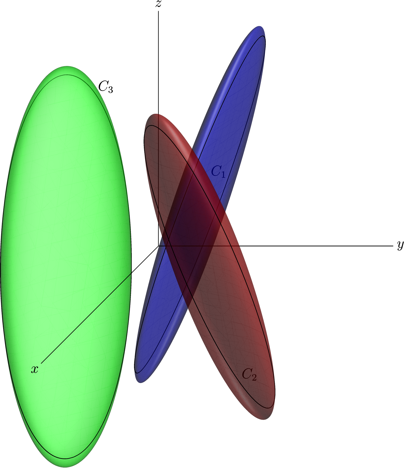
Figure 1. Isometric spheres of the $\iota_{i}$ reflections for $\mathscr{S}$.

Let $\iota_{0},\iota_{1},\iota_{2}$ the complex reflections induced by these complex chains, an straight computation shows that

$$\det\left(\frac{\partial\iota_{i}}{\partial(\zeta,v)}(t)\right)=\frac{|\sin^{4}(\theta)|}{12}.$$

The transition matrix is given by

$$T=\frac{1}{12}\left(\begin{array}[]{ccc}0&k(\theta)^{4}&k(\theta)^{4}\\ k(\theta)^{4}&0&k(\theta)^{4}\\ k(\theta)^{4}&k(\theta)^{4}&0\end{array}\right)$$

The eigenvalue of $T^{\alpha}$ have to satisfy $2\left(\frac{k(\theta)^{4}}{12}\right)^{\alpha}=1,$ so

$$\alpha=\frac{\log(2)}{\log(12)-4\log(k(\theta))}.$$

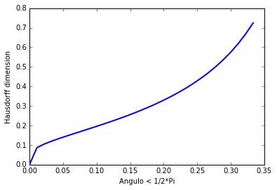
Figure 2. The computed Hausdorff dimension for $\Lambda_{CG}(\Gamma(\mathscr{S}))$ varying $\theta.$

As the action of a Schottky group defined by complex chains contained in $\mathfrak{H}\times\{0\}$ is like the classic Schottky group action on $\mathbb{H}^{2},$ we can see the analog of the example computed in [16], as you can see in Figure 2.

Example 3.7 (Non-Symmetric $\theta-$Schottky groups.).

We can put the generating chains’ center in any part of the Heisenberg space; if we place these centers close to points in the standard finite $\mathbb{R}-$circle, more precisely on $\sec(\theta)(0,1),\sec(\theta)(0,-1)$ and $\sec(\theta)(-i,0),$ we can construct a $\theta-$Schottky group but instead of the angle belongs to $(0,\pi/3),$ we have to ask that the angle belongs to $(0,9\pi/40),$ this is to guarantee the convex cocompact property on the group.

Since the standard finite $\mathbb{R}-$circle is a space circle whose planar projection is a lemniscate, we loose the symmetry on the chains and the centers. Let $\mathscr{C}$ denote the collection of the following three chains parametrized by

$$t \mapsto \left(\tan(\theta)e^{it},\sec^{2}(\theta)\right)$$

$$t \mapsto \left(\tan(\theta)e^{it},-\sec^{2}(\theta)\right)$$

$$t \mapsto \left(\tan(\theta)e^{it}-i\sec(\theta),-2\sec(\theta)\tan(\theta)\cos(t)\right)$$

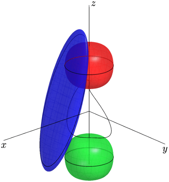
Figure 3. Configuration of three finite chains that generate a $\theta-$Schottky Group

We denote by $\hat{\iota}_{i}$ the complex reflections generated by the previous chains, and a straight computations shows that the analysis done for the previous groups holds for these groups. For this reason if we took a set of uniformly distributed angles on $(0,9\pi/40)$ the Hausdorff dimension of its Chen-Greenberg limit set behave similarly as you can see in the following figure.

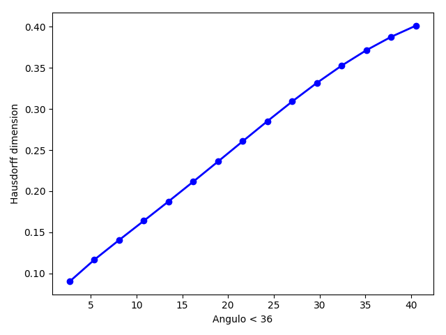
Figure 4. The computed Hausdorff dimension for $\Lambda_{CG}(\Gamma(\mathscr{C}))$ varying $\theta.$

Appendix A Pseudo-code for the McMullen Algorithm

The algorithm was implemented in Python and is combination of the eigenvalue algorithm (see [16]) and the Newton method (see [11]). The algorithm is subdivided into function pieces, each of these pieces are used in the global function.

1

2function Inversion$(c,r,\zeta)$;

Input : $c-$ array of the center of the complex chain.

$r-$ multiplier of the reflection, $|r|$ is the radious of the complex chain.

$\zeta-$ array of a point in Heisenberg different from $\infty.$

Output : $z-$ array of a point Heisenberg coordinates.

3 $z[1]=c[1]-\frac{|r|^{2}(\zeta[1]-c[1])(|\zeta[1]-c[1]|^{2}+i(\zeta[2]-c[2]-2Im(\overline{\zeta[1]}c[1])))}{|\zeta[1]-c[1]|^{4}+(\zeta[2]-c[2]-2Im(\overline{\zeta[1]}c[1]))^{2}}$;

4 $z[2]=c[2]-\frac{|r|^{4}(\zeta[2]-c[2]-2Im(\overline{\zeta[1]}c[1]))+2|r|^{2}Im(\overline{-(\zeta[1]-c[1])(|\zeta[1]-c[1]|^{2}+i(\zeta[2]-c[2]-2Im(\overline{\zeta[1]}c[1]))\zeta[1])})}{|\zeta[1]-c[1]|^{4}+(\zeta[2]-c[2]-2Im(\overline{\zeta[1]}c[1]))^{2}}$;

return $z$

Algorithm 1 Complex reflection defined by a complex chain in Heisenberg coordinates

1

2function words$(k,m,reflex)$;

Input : $k-$ maximal depth of the Word tree, nonnegative integer

$m-$ number of reflections, nonnegative integer

$reflex-$ array of $m$ points in $\mathfrak{H}\times(\mathbb{C}\setminus\{0\})$.

Output : $w-$ array of tagpoints

$wordsN-$ array of characters of words in the Tree of lenght $k-1.$

3 $N=m*(m-1)^{k-1}$;

4 $tagpoints=array([30000000])$;

5 $words=array([3000000])$;

6 for $i=1,\cdots,m$ do

      $tagpoints[i]=reflex[i][1]-\epsilon$ ;

        // $\epsilon$ small

7      

8 end for

9$inv=array[1,2,\cdots,m]$;

10 $tag=zeros[3000000]$;

11 $num=zeros[k+2]$;

12 for $i=1,\cdots,m$ do

13      $tag[i]=i$;

14       $words[i]=`i^{\prime}$

15 end for

16$num[1]=1$;

17 $num[2]=m+1$;

18 for $lev=2,\cdots,k+2$ do

19      $inew=num[lev]$;

20       for $j=1,\cdots,m$ do

21             for $iold=num[lev-1],\cdots,num[lev]$ do

22                   if $j=inv[tag[iold]]$ then

23                        CONTINUE

24                   end if

25                  else

26                        $tagpoints[inew]=Inversion(reflex[j],tagpoints[iold])$;

27                         $words[inew-1]=words[j]+words[iold]$;

28                         $tag[inew]=j$;

29                         $inew=+1$;

30                   end if

31                  

32             end for

33            $num[lev]=inew$;

34       end for

35      

36 end for

37for $i=1,\cdots,num[k]-num[k-1]$ do

38      $w[i]=tagpoints[num[k]]+i]$

39 end for

40for $i=1,\cdots,num[k-1]-num[k-2]$ do

41      $wordsN[i]=words[num[k]+i]$

42 end for

return $w,wordsN$

Algorithm 2 Tagpoints and Words (see [17])

1

2function NewtonHausdorff$(d,T,\varepsilon)$;

Input : $d-$ stimated value for the Hausdorff dimension (usual valor 1).

$T-$ a transition matrix.

$\varepsilon-$ desired error.

Output : $dHauss-$ aproximated value for the Hausdorff dimension.

3 $N=RankT$;

4 $aNew=d$;

5 $x=ones[N]/N$;

6 $x0=x$;

7 while $cont<350$ do

8       $Td=T^{aNew}$;

9       $a,x=PerronFrobenious(N,Td,x)$;

10       if $|a-1|<\varepsilon$ then

11             BREAK;

12       end if

13      else

14             $d0=d+0.1$;

15             $TdE=T^{d0}$;

16             $aE,xE=PerronFrobenious(N,TdE,x0)$;

17             $Der=(aE-a)/0.01$;

18             $aNew=d+(1-a)/Der$;

19             $d=aNew$;

20             if $|d-1|<\varepsilon$ then

21                  BREAK

22             end if

23            else

24                  $cont=+1$

25             end if

26            

27       end if

28      

29 end while

return $d$

Algorithm 3 The Newton algorithm for the approximation of Hausdorff dimension

References

- [1] P. Albuquerque, Patterson-Sullivan theory in higher rank symmetric spaces, Geom. Funct. Anal. 9 (1999), no. 1, 1–28.
- [2] James W Anderson and André C Rocha, Analyticity of hausdorff dimension of limit sets of kleinian groups, ANNALES-ACADEMIAE SCIENTIARUM FENNICAE SERIES A1 MATHEMATICA, vol. 22, ACADEMIA SCIENTIARUM FENNICA, 1997, pp. 349–364.
- [3] Nadia Benakli and Ilya Kapovich, Boundaries of hyperbolic groups, Contemporary Mathematics 296 (2002), 39–94.
- [4] Brian H Bowditch et al., Geometrical finiteness with variable negative curvature, Duke Mathematical Journal 77 (1995), no. 1, 229–274.
- [5] Martin Bridgeman, Richard Canary, François Labourie, and Andres Sambarino, The pressure metric for anosov representations, Geometric and Functional Analysis 25 (2015), no. 4, 1089–1179.
- [6] Angel Cano, Juan Pablo Navarrete, and José Seade, Complex kleinian groups, Complex Kleinian Groups, Springer, 2013, pp. 77–92.
- [7] J-P Conze and Yves Guivarc’H, Limit sets of groups of linear transformations, Sankhyā: The Indian Journal of Statistics, Series A (2000), 367–385.
- [8] Michel Coornaert, Mesures de Patterson-Sullivan sur le bord d’un espace hyperbolique au sens de Gromov, Pacific J. Math. 159 (1993), no. 2, 241–270.
- [9] Michel Coornaert and Athanase Papadopoulos, Spherical functions and conformal densities on spherically symmetric cat(-1)-spaces, Transactions of the American Mathematical Society 351 (1999), no. 7, 2745–2762.
- [10] Laurent Dufloux, Hausdorff dimension of limit sets, Geometriae Dedicata 191 (2017), no. 1, 1–35.
- [11] Lucy Garnett, A computer algorithm for determining the hausdorff dimension of certain fractals, Mathematics of computation 51 (1988), no. 183, 291–300.
- [12] William M Goldman and John R Parker, Complex hyperbolic ideal triangle groups, J. reine angew. Math 425 (1992), 71–86.
- [13] William Mark Goldman, Complex hyperbolic geometry, Oxford University Press, 1999.
- [14] Olivier Guichard and Anna Wienhard, Anosov representations: domains of discontinuity and applications, Inventiones mathematicae 190 (2012), no. 2, 357–438.
- [15] Sa’ar Hersonsky and Frédéric Paulin, Diophantine approximation in negatively curved manifolds and in the heisenberg group, Rigidity in dynamics and geometry, Springer, 2002, pp. 203–226.
- [16] Curtis T McMullen, Hausdorff dimension and conformal dynamics, iii: Computation of dimension, American journal of mathematics 120 (1998), no. 4, 691–721.
- [17] David Mumford, Caroline Series, and David Wright, Indra’s pearls, Cambridge University Press, New York, 2002, The vision of Felix Klein.
- [18] John R Parker, On ford isometric spheres in complex hyperbolic space, Mathematical Proceedings of the Cambridge Philosophical Society, vol. 115, Cambridge University Press, 1994, pp. 501–512.
- [19] by same author, Notes on complex hyperbolic geometry, (2003).
- [20] S. J. Patterson, The limit set of a Fuchsian group, Acta Math. 136 (1976), no. 3-4, 241–273.
- [21] Jean-François Quint, An overview of patterson-sullivan theory, Workshop The barycenter method, FIM, Zurich, 2006.
- [22] Richard Evan Schwartz, A better proof of the goldman–parker conjecture, Geometry & Topology 9 (2005), no. 3, 1539–1601.
- [23] Dennis Sullivan, The density at infinity of a discrete group of hyperbolic motions, Publications Mathématiques de l’Institut des Hautes Études Scientifiques 50 (1979), no. 1, 171–202.
- [24] by same author, Entropy, hausdorff measures old and new, and limit sets of geometrically finite kleinian groups, Acta Mathematica 153 (1984), no. 1, 259–277.