The Newcomb–Benford law: Scale invariance and a simple Markov process based on it

Abstract

The Newcomb–Benford law, also known as the first-digit law, gives the probability distribution associated with the first digit of a dataset, so that, for example, the first significant digit has a probability of $30.1$ % of being $1$ and $4.58$ % of being $9$. This law can be extended to the second and next significant digits. This article presents an introduction to the discovery of the law, its derivation from the scale invariance property, as well as some applications and examples. Additionally, a simple model of a Markov process inspired by scale invariance is proposed. Within this model, it is proved that the probability distribution irreversibly converges to the Newcomb–Benford law, in analogy to the irreversible evolution toward equilibrium of physical systems in thermodynamics and statistical mechanics.

I Introduction

In the late 19th century, an astronomer and mathematician visits his institution’s library and consults a table of logarithms to perform certain astronomical calculations. As on previous occasions, he is struck by the fact that the first pages (those corresponding to numbers that start at $1$) are much more worn than the last ones (corresponding to numbers that start at $9$). Intrigued, this time he decides not to overlook the matter. He closes his eyes to concentrate, sketches a few calculations on a piece of paper, and finally smiles. He has found the answer and it turns out to be enormously simple and elegant.

A little over half a century later, a physicist and electrical engineer who is unaware of his predecessor’s discovery, observes the same curious phenomenon on the pages of logarithm tables, and arrives at the same conclusion. Both have understood that, in a long list of records $\{r_{n}\}$ obtained from measurements or observations, the fraction $p_{d}$ of records beginning with the significant digit $d=1,2,\ldots,9$ is not $p_{d}=1/9$, as one might naively expect, but rather follows a logarithmic law. More specifically,

$$p_{d}=\log_{10}\left(1+\frac{1}{d}\right),\quad d=1,2,\ldots,9.$$ (1)

The numeric values of $p_{d}$ are shown in the second column of Table 1. We see that the records that start with $1$, $2$, or $3$ account for around $60$ % of the total, while the other six digits must settle for the remaining $40$ %.

Table 1: Probabilities for the first, second, third, and fourth significant digits.

Digit	First	Second	Third	Fourth
$d$	$p_{d}$	$p_{d}^{(2)}$	$p_{d}^{(3)}$	$p_{d}^{(4)}$
$0$	$\cdots$	$0.119\,68$	$0.101\,78$	$0.100\,18$
$1$	$0.301\,03$	$0.113\,89$	$0.101\,38$	$0.100\,14$
$2$	$0.176\,09$	$0.108\,82$	$0.100\,97$	$0.100\,10$
$3$	$0.124\,94$	$0.104\,33$	$0.100\,57$	$0.100\,06$
$4$	$0.096\,91$	$0.100\,31$	$0.100\,18$	$0.100\,02$
$5$	$0.079\,18$	$0.096\,68$	$0.099\,79$	$0.099\,98$
$6$	$0.066\,95$	$0.093\,37$	$0.099\,40$	$0.099\,94$
$7$	$0.057\,99$	$0.090\,35$	$0.099\,02$	$0.099\,90$
$8$	$0.051\,15$	$0.087\,57$	$0.098\,64$	$0.099\,86$
$9$	$0.045\,76$	$0.084\,90$	$0.098\,27$	$0.099\,82$

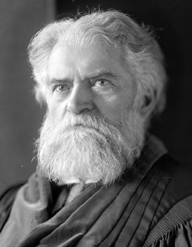
Figure 1: Simon Newcomb (1835–1909).

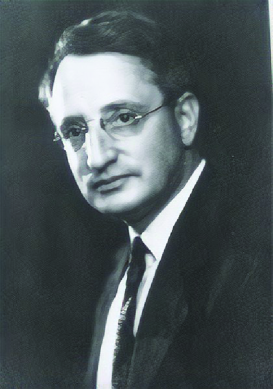
Figure 2: Frank Benford (1883–1948).

Our 19th century character is Simon Newcomb (Fig. 1) and he published his discovery in a modest two-page note.[1] The second character is Frank Benford (Fig. 2) and he wrote a $22$-page article[2] in which, in addition to mathematically justifying Eq. (1), he showed its validity in the analysis of more than $20\,000$ first digits taken from sources as varied as river areas, populations of American cities, physical constants, atomic and molecular weights, specific heats, numbers taken from newspapers or Reader’s Digest, postal addresses, …, and the series $n^{-1}$, $\sqrt{n}$, $n^{2}$, or $n!$, among others, with $n\in\llbracket 1,100\rrbracket$.

With such an overwhelming evidence, it is not surprising that Eq. (1) is usually known as Benford’s law (or first-digit law), even though it was found nearly sixty years earlier by Newcomb. This is one more manifestation of the so-called Stigler’s law, according to which no scientific discovery is named after the person who discovered it in the first place. In fact, as Stigler himself points out,[3] the law that bears his name was actually spelled out in a similar way twenty-three years earlier by the American sociologist Robert K. Merton. In order not to fall completely into Stigler’s law, many authors refer to Eq. (1) as Newcomb–Benford’s law and that is the convention (by means of the acronym NBL) that we will follow in this article.

While the literature on the NBL in specialized journals is vast,[4] and several books on the topic are available,[5, 6, *M15, *K15, *K19, *N20] the number of papers in general or science education journals is much scarcer.[11, *FH45, *L86, *BK91, *P02, *TFGS07, *F09, *MA18, *L19, 20, 21] In this paper, apart from revisiting the NBL and illustrating it with a few examples, we construct a Markov-chain model inspired by the invariance property of the NBL under the operation of a change of scale.

The remainder of the paper is organized as follows. The connection between the NBL (and some of its generalizations) with the property of scale invariance is formulated in Sec. II. This is followed by a few examples in Sec. III. The most original part is contained in Sec. IV, where our Markov-chain model is proposed and solved. Finally, the paper is closed in Sec. V with some concluding remarks. For the interested reader, Appendices A–C contain the most technical and mathematical parts of Secs. II and IV.

II Origin of the law

Often times, when one first speaks to a friend, relative, or even a colleague about the NBL, their first reaction is usually of skepticism. Why is the first digit not evenly distributed among the nine possible values? A simple argument shows that, if a robust distribution law exists, it cannot be the uniform distribution whatsoever.

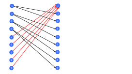
Figure 3: Diagram showing how the first digit changes when all the records of a dataset are doubled.

Imagine a long list of river lengths, mountain heights, and country surfaces, for example. It is possible that the lengths of the rivers are in km, the heights of the mountains in m, and the surfaces of countries in $\text{km}^{2}$, but they could also be expressed in miles, feet, or acres, respectively. Will the distribution $p_{d}$ depend on whether we use some units or others, or even if we mix them? It seems logical that the answer should be negative; that is, the $p_{d}$ distribution should be (statistically) independent of the units chosen; in other words, it is expected that the $p_{d}$ distribution is invariant under a change of scale. The uniform distribution $p_{d}=\frac{1}{9}$ obviously does not follow that property of invariance. Suppose we start from a dataset in which all the values of the first digit are equally represented. If we multiply all the records in the dataset by $2$, we can see that those records that started before with $1$, $2$, $3$, and $4$ then start with either $2$ or $3$, either $4$ or $5$, either $6$ or $7$, and either $8$ or $9$, respectively. On the other hand, all those that started with $5$, $6$, $7$, $8$, or $9$ start now with $1$. All those possibilities are schematically shown in Fig. 3. Therefore, if $p_{d}=\frac{1}{9}$ initially, then $p_{1}=\frac{5}{9}$ and $p_{2}+p_{3}=p_{4}+p_{5}=p_{6}+p_{7}=p_{8}+p_{9}=\frac{1}{9}$ after doubling all the records, thus destroying the initial uniformity.

Thus, the most identifying hallmark of the NBL is that it must be applied to records that have units or, as Newcomb himself writes,[1] “As natural numbers occur in nature, they are to be considered as the ratios of quantities.”

While relatively formal mathematical proofs of the NBL can be found in the literature,[22, *F66, *R69, *R76, *D77, *N84, *H95b, *LSE00, *CLM19, *CM19, *V20, *BH20, 34, 35] in Appendix A, we present a sketch of a simpler, physicist-style derivation of the law by imposing invariance under a change of scale.[36]

Equation (1) can be generalized beyond the first digit. The probability that the $m$ first digits of a record match the ordered string $(d_{1},d_{2},\ldots,d_{m})$, where $d_{1}\in\{1,2,\ldots,9\}$ and $d_{i}\in\{0,1,2,\ldots,9\}$ if $i\geq 2$, is given by (see Appendix A)

$$p_{d_{1},d_{2},\ldots,d_{m}}=\log_{10}\left[1+\left(\sum_{i=1}^{m}d_{i}\times 10^{m-i}\right)^{-1}\right].$$ (2)

As an example, the probability that the first three digits of a record form precisely the string $(3,1,4)$ is $p_{3,1,4}=\log_{10}\left(1+{1}/{314}\right)=0.001\,38$.

Once we have $p_{d_{1},d_{2},\ldots,d_{m}}$, we can calculate the probability $p_{d}^{(m)}$ that the $m$th digit is $d$, regardless of the values of the preceding $m-1$ digits, just by summing for all possible values of those preceding $m-1$ digits,

$$p_{d}^{(m)}=\sum_{d_{1}=1}^{9}\sum_{d_{2}=0}^{9}\cdots\sum_{d_{m-1}=0}^{9}p_{d_{1},d_{2},\ldots,d_{m-1},d}.$$ (3)

In Table 1, the law for the first digit, $p_{d}$, is accompanied by the laws for the second, third, and fourth digits, obtained from Eqs. (2) and (3). As the digit moves to the right, the probability distribution becomes less and less disparate.

In Fig. 3 we saw that, when multiplying a dataset $\{r_{n}\}$ by $2$, part of the records that started with $d=1,2,3,4$, specifically those that start with the first two digits $(d,0)$, $(d,1)$, $(d,2)$, $(d,3)$, or $(d,4)$, will start with $2d$, while the rest will start with $2d+1$. Let us call $\alpha_{d}$ the fraction of records that, initially starting with $d=1,2,3,4$, start with $2d$ by doubling all the records. Thus,

$$\alpha_{d}=\frac{\sum_{d_{2}=0}^{4}p_{d,d_{2}}}{p_{d}},\quad d=1,2,3,4.$$ (4)

If the dataset fulfills the NBL, then one has

$$\alpha_{1}= \frac{\log_{10}\dfrac{3}{2}}{\log_{10}2}\simeq 0.584\,96,\quad\alpha_{2}=\frac{\log_{10}\dfrac{5}{4}}{\log_{10}\dfrac{3}{2}}\simeq 0.550\,34,$$ (5a)

$$\alpha_{3}= \frac{\log_{10}\dfrac{7}{6}}{\log_{10}\dfrac{4}{3}}\simeq 0.535\,84,\quad\alpha_{4}=\frac{\log_{10}\dfrac{9}{8}}{\log_{10}\dfrac{5}{4}}\simeq 0.527\,84.$$ (5b)

We will use these values later in Sec. IV.

III Applications and examples

The applications and verifications of the NBL are numerous and cover topics as varied and prosaic as the study of the genome,[37] atomic,[38] nuclear,[20, 39, *NWR09] and particle[41, *DD18] physics, astrophysics,[43, *SM10a, *AL14, *HF16, *SPP17, *JBR20] quantum correlations,[49, *BMRBSS18, *BDSRSS18] toxic emissions,[52] biophysics,[53] medicine,[54] dynamical systems,[55, *SCD01, *BBH04] distinction of chaos from noise,[58] statistical physics,[59] scientific citations,[60, *AYS14] tax audits,[62, 5] electoral[63, *R14, *GA18] or scientific[66] frauds, gross domestic product,[67, *AEKD19] stock market,[21, 69] inflation data,[70] climate change,[71] world wide web,[72] internet traffic,[73] social networks,[74] textbook exercises,[75] image processing,[76] religious activities,[77, *M14, *A14] dates of birth,[80] hydrology and geology,[81, *STJ10, *GM12, *ACL17] fragmentation processes,[85, *BBCGIJMPRSST18] the first letters of words,[87] or even COVID-19.[88, *KY20] Other examples can be seen in the link of Ref. 90. In this section, we will present some additional examples.

Let us start with one of the situations that Benford himself studied in his classic paper:[2] city populations. Using data from the Spanish National Institute of Statistics,[91] we have considered the 2019 population of the $165$ municipalities in the province of Badajoz (plus the total population of the province of Badajoz), of the $223$ municipalities of the province of Cáceres (plus the total population of the province of Cáceres), and the total population of the $388$ municipalities of the Spanish region of Extremadura, which encompasses the provinces of Badajoz and Cáceres, (plus the total populations of the provinces of Badajoz and Cáceres). We have also considered the population (according to the $2016$ census) of the $8\,110$ Spanish municipalities. For all these lists of records, we have analyzed the frequency of those starting with $d=1,2,\ldots 9$ and the results are compared in Fig. 4. There is a good general agreement between the population data and the NBL predictions. This is interesting, since it is not obvious that the distribution of the number of inhabitants of municipalities should be invariant under a change of scale.

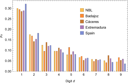
Figure 4: Histograms showing the distribution of the first digit for (from left to right at each digit $d$) the NBL and the populations of the municipalities of the provinces of Badajoz and Cáceres, the region of Extremadura, and Spain.

Let us now turn to two examples from astronomy. In the first one, we take the distance from Earth (in light-years and in parsecs) to the $300$ brightest stars.[92] In the second case, the data are the daily number of sunspots from $1818$ to the present.[93] As seen in Fig. 5, the distances between our planet and the $300$ brightest stars agree reasonably well with the NBL, despite the fact that the list is not excessively long (only $300$ data points) and that there are “local” deviations (for example, $p_{6}<p_{7}$ in the two choices of units). This general agreement was to be expected, since the distribution of digits in distances (which are expressed in units) is a clear example of invariance under a change of scale. However, in the case of the daily number of sunspots, quantitative (although not qualitative) differences are observed with the NBL, especially in the $d=1$, $3$, $4$, and $5$ cases. It should be noted that, although the series is rather long (more than $59\,000$ records, after excluding days without data or with zero spots), each record only has one, two, or three digits (the maximum number of sunspots was $528$ and corresponded to August 26, 1870), thus producing a certain bias to records starting with $1$. Moreover, the daily number of sunspots cannot be expressed in units and therefore may not be scale-invariant.

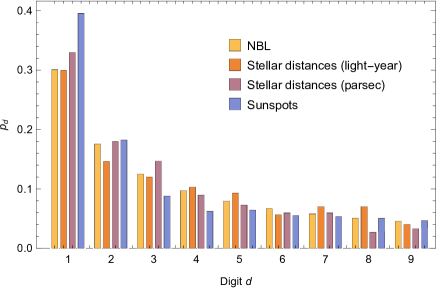
Figure 5: Histograms showing the distribution of the first digit for (from left to right at each digit $d$) the NBL, the distances to Earth in light-years and in parsecs from the brightest $300$ stars, and the daily number of sunspots.

Finally, we have analyzed the prices of $1\,016$ items from a chain of fashion retailers [94] and of $1\,373$ products from a chain of hypermarkets [95]. The results are shown in Fig. 6. In this case, the discrepancies with the NBL are more pronounced. Although the highest frequencies occur for $d=1$ and $d=2$, the observed values of $p_{d}$ do not decrease monotonically with increasing $d$. In the case of the fashion retailers, we have $p_{4}>p_{3}$ and $p_{9}>p_{8}>p_{6}>p_{7}$; in the prices of the chain of hypermarkets, $p_{8}>p_{9}>p_{7}>p_{6}$. In principle, one might think that, since they can be expressed in euro, pound, dollar, peso, ruble, yen, …, prices should satisfy the property of invariance under a change of scale inherent to the NBL. However, commercial and artificial pricing strategies must be superimposed on this invariance, which generates relevant deviations with respect to the NBL.

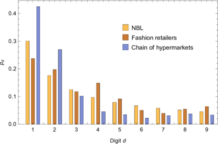
Figure 6: Histograms showing the distribution of the first digit for (from left to right at each digit $d$) the NBL and the prices of articles of a chain of fashion retailers and a chain of hypermarkets.

IV A simple model of a Markov chain based on the scale invariance property of the Newcomb–Benford distribution

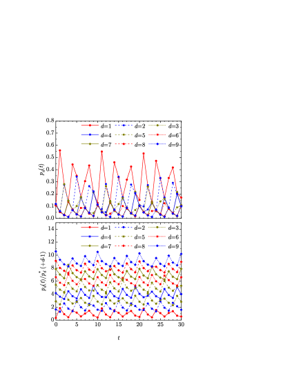
Figure 7: Evolution of the first-digit distribution $p_{d}(t)$ (top panel) and of the ratio $p_{d}(t)/p_{d}^{*}$ (bottom panel, where a vertical shift $d-1$ has been applied for better clarity), $\{p_{d}^{*}\}$ being the NBL distribution, when starting from a dataset of $10^{4}$ random records uniformly distributed between $0$ and $1$ and doubling the records at each time step. Note the overlap of some of the points in the top panel.

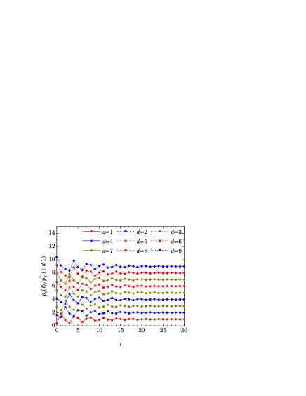
Figure 8: Evolution of the ratio $p_{d}(t)/p_{d}^{*}$ (where a vertical shift $d-1$ has been applied for better clarity), when starting from a uniform initial distribution $p_{d}(0)=\frac{1}{9}$, according to our Markov-chain model, Eq. (7).

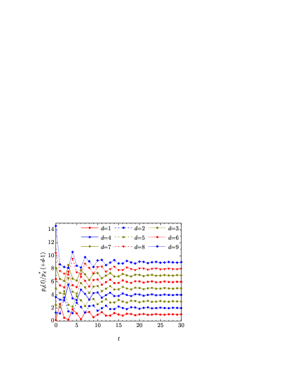
Figure 9: Evolution of the ratio $p_{d}(t)/p_{d}^{*}$ (where a vertical shift $d-1$ has been applied for better clarity), when starting from an inverted initial distribution $p_{d}(0)=p_{10-d}^{*}$, according to our Markov-chain model, Eq. (7).

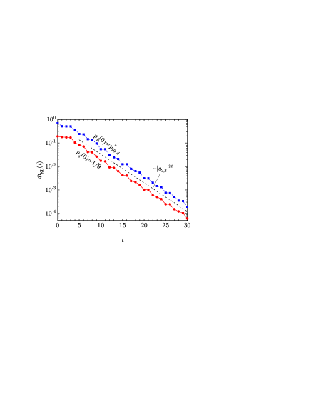
Figure 10: Evolution of the Kullback–Leibler divergence $\mathcal{D}_{\text{KL}}(t)$ (in logarithmic scale), starting from the uniform initial distribution $p_{d}(0)=\frac{1}{9}$ and from the inverted initial distribution $p_{d}(0)=p_{10-d}^{*}$, according to our Markov-chain model, Eq. (7). The dashed line is proportional to $|a_{2,3}|^{2t}$ (see Appendix C).

As already said, NBL, Eq. (1), is invariant under a change of scale; that is, if we start from a dataset $\{r_{n}\}$ that fulfills the NBL and multiply all the records by a constant $\lambda$, the resulting dataset $\{\lambda r_{n}\}$ still fulfills the NBL.

It is tempting to conjecture that the NBL should be an attractor of this process. This would mean that, if we started from an initial dataset $\{r_{n}(0)\}$ that does not fulfill the NBL and generated new sets $\{r_{n}(t)\}=\{\lambda^{t}r_{n}(0)\}$ at times $t=1,2,\ldots$ by multiplying each successive dataset by $\lambda$ (other than a fractional power of $10$), the first-digit distribution $\{p_{d}(t)\}$ of the generated sets would converge toward the NBL. However, this is not the case. As illustrated in Fig. 7 for the case $\lambda=2$ and an initial dataset of $10^{4}$ random numbers, the time-dependent distribution $\{p_{d}(t)\}$ exhibits a quasiperiodic oscillatory pattern around the NBL distribution without any apparent amplitude attenuation. In fact, since $2^{10}=1\,024\simeq 10^{3}$, the distribution nearly returns to the uniform initial one at times $t=10,20,30,\ldots$. This behavior is reminiscent of the Poincaré recurrence time in mechanical systems and the associated Zermelo paradox about irreversibility.[96]

In the transformation $\{r_{n}(t)\}\to\{r_{n}(t+1)=2r_{n}(t)\}$, the first-digit distribution changes, according to Fig. 3, as

$$p_{1}(t+1)=p_{5}(t)+p_{6}(t)+p_{7}(t)+p_{8}(t)+p_{9}(t),$$ (6a)

$$p_{2}(t+1)=\alpha_{1}p_{1}(t),\quad p_{3}(t+1)=(1-\alpha_{1})p_{1}(t),$$ (6b)

$$p_{4}(t+1)=\alpha_{2}p_{2}(t),\quad p_{5}(t+1)=(1-\alpha_{2})p_{2}(t),$$ (6c)

$$p_{6}(t+1)=\alpha_{3}p_{3}(t),\quad p_{7}(t+1)=(1-\alpha_{3})p_{3}(t),$$ (6d)

$$p_{8}(t+1)=\alpha_{4}p_{4}(t),\quad p_{9}(t+1)=(1-\alpha_{4})p_{4}(t),$$ (6e)

where the fractions $\alpha_{d}$ ($d=1,2,3,4$) are defined by Eq. (4). Note that, in general, the fractions $\alpha_{d}$ depend on the distributions of the first digit, $p_{d}(t)$, and of the first two digits, $p_{d,d_{2}}(t)$, of the dataset $\{r_{n}(t)\}$ [see Eq. (4)]. As a consequence, (i) Eqs. (6) do not make a closed set and (ii) the parameters $\alpha_{d}$ depend on $t$.

At this point, we construct a simplified dynamical model in which the four unknown and time-dependent parameters $\alpha_{d}$ in Eqs. (6) are replaced by fixed constants. In matrix notation,

$$\bm{p}(t+1)=\mathsf{W}\cdot\bm{p}(t),$$ (7)

where ${\bm{p}}(t)=\left(p_{1}(t),p_{2}(t),\ldots,p_{9}(t)\right)^{\dagger}$ is a column vector ($\dagger$ denotes transposition) and

$$\mathsf{W}=\begin{pmatrix}0&0&0&0&1&1&1&1&1\\ \alpha_{1}&0&0&0&0&0&0&0&0\\ 1-\alpha_{1}&0&0&0&0&0&0&0&0\\ 0&\alpha_{2}&0&0&0&0&0&0&0&\\ 0&1-\alpha_{2}&0&0&0&0&0&0&0&\\ 0&0&\alpha_{3}&0&0&0&0&0&0&\\ 0&0&1-\alpha_{2}&0&0&0&0&0&0&\\ 0&0&0&\alpha_{4}&0&0&0&0&0&\\ 0&0&0&1-\alpha_{4}&0&0&0&0&0&\\ \end{pmatrix}$$ (8)

is a fixed square matrix. Equation (7) fits the canonical description of Markov chains,[97] where $\mathsf{W}$ is the so-called transition matrix, and $\{\alpha_{d}\}$ correspond to transition probabilities. In this way, we may forget about the meaning of $\{p_{d}(t)\}$ as the first-digit distribution of the dataset $\{r_{n}(t)\}$ and look at the numerals $1,2,\ldots,9$ as labels of nine distinct internal states of a certain physical system which follow each other in the prescribed order sketched by Fig. 3.

Note that the matrix $\mathsf{W}$ is singular, that is, not invertible. This implies the irreversible character of the transition $\{p_{d}(t)\}\to\{p_{d}(t+1)\}$. The stationary solution $\bm{p}^{*}$ to Eq. (7) satisfies the condition $\bm{p}^{*}=\mathsf{W}\cdot\bm{p}^{*}$. Such a stationary solution will be an attractor of our Markov process if $\lim_{t\to\infty}\bm{p}(t)=\bm{p}^{*}$ for any initial condition $\bm{p}(0)$. This property, along with the exact solution of Eq. (7), is proved in Appendix B. If we choose for $\alpha_{d}$ the values given by Eqs. (5), the stationary solution coincides exactly with the NBL, as could be expected. This will be the choice made in the rest of this section.

To illustrate the irreversible evolution of $\bm{p}(t)$ toward $\bm{p}^{*}$, we are going to consider two different initial conditions. First, we start from a uniform distribution, that is, $p_{d}(0)=\frac{1}{9}$. The result is shown in Fig. 8, where we see that the evolution is oscillatory (see Appendix B for an explanation) and the oscillations are rapidly damped to attain the stationary solution. As a second example, we take an NBL inverted initial distribution, that is, $p_{d}(0)=p_{10-d}^{*}$, so that, initially, state $9$ is the most probable and state $1$ is the least probable. In this second example, as shown in Fig. 9, the initial oscillations are of greater amplitude but, as before, the stationary distribution is practically reached after a few iterations. Comparison between Figs. 7 and 8 shows that the main difference between our Markov model and the non-Markovian evolution of $\{p_{d}(t)\}$ in a real dataset is that the oscillation amplitudes are attenuated in the model and not in the original framework.

It seems convenient to characterize the evolution of the set of probabilities $\{p_{d}(t)\}$ obeying the Markov process [Eq. (7)] toward the attractor $\{p_{d}^{*}\}$ by means of a single parameter that, in addition, evolves monotonically, thus representing the irreversibility of evolution. It is expected that these properties are verified by the Kullback–Leibler divergence,[98] which in our case is defined as

$$\mathcal{D}_{\text{KL}}(t)=\sum_{d=1}^{9}p_{d}(t)\ln\frac{p_{d}(t)}{p_{d}^{*}}.$$ (9)

This quantity represents the opposite of the Shannon entropy[99] of $\{p_{d}(t)\}$, except that it is measured with respect to the stationary distribution $\{p_{d}^{*}\}$. In the context of our Markov-chain model, $\mathcal{D}_{\text{KL}}$ is related to information theory. On the other hand, the mathematical structure of $\mathcal{D}_{\text{KL}}$ can be extended to physical systems, thus providing a statistical-mechanical basis to the thermodynamic entropy,[99, 100] as exemplified below.

Figure 10 shows the evolution of $\mathcal{D}_{\text{KL}}(t)$ for the same initial conditions as in Figs. 8 and 9. Both cases confirm the desired monotonic evolution of $\mathcal{D}_{\text{KL}}(t)$. Also, the asymptotic decay $\mathcal{D}_{\text{KL}}(t)\to 0$ occurs essentially exponentially with a rate independent of the initial probability distribution. This is proved in Appendix C, as well as the monotonicity property

$$\mathcal{D}_{\text{KL}}(t+1)\leq\mathcal{D}_{\text{KL}}(t),$$ (10)

with the equality not holding for two successive times unless $p_{d}(t)=p_{d}^{*}$, in which case $\mathcal{D}_{\text{KL}}=0$.

Table 2: Analogy between a classical dilute gas (as a prototypical physical system) and a system described by the Markov chain, Eq. (7). In the expression of the Maxwell–Boltzmann distribution $f_{\text{MB}}(\vec{v})$, $m$ is the mass of a molecule, $T$ is the gas temperature, and $k_{B}$ is the Boltzmann constant. In the Boltzmann equation, $J[\vec{v}|f(t),f(t)]$ is the collision operator.

	Dilute gas	Markov chain
Probability distribution	Velocity distribution function: $f(\vec{v},t)$	Probability of the internal state $d$: $p_{d}(t)$
Normalization	$\displaystyle{\int\text{d}^{3}\vec{v}\,f(\vec{v},t)=1}$	$\displaystyle{\sum_{d=1}^{9}p_{d}(t)=1}$
Evolution equation	Boltzmann equation: $\displaystyle{\frac{\partial f(\vec{v},t)}{\partial t}=J[\vec{v}|f(t),f(t)]}$	$\displaystyle{\bm{p}(t+1)=\mathsf{W}\cdot\bm{p}(t)}$
Equilibrium state	Maxwell–Boltzmann: $\displaystyle{f_{\text{MB}}(\vec{v})=\left(\frac{m}{2\pi k_{B}T}\right)^{3/2}\text{e}^{-mv^{2}/2k_{B}T}}$	NBL: $p_{d}^{*}=\log_{10}\left(1+d^{-1}\right)$
Entropy functional	$\displaystyle{S(t)=-\int\text{d}^{3}\vec{v}\,f(\vec{v},t)\ln\frac{f(\vec{v},t)}{f_{\text{MB}}(\vec{v})}}$	$\displaystyle{S(t)=-\sum_{d=1}^{9}p_{d}(t)\ln\frac{p_{d}(t)}{p_{d}^{*}}}$
Irreversibility equation	$\displaystyle{\frac{\text{d}S(t)}{\text{d}t}\geq 0}$	$\displaystyle{S(t+1)-S(t)\geq 0}$

Thus, we can say that the NBL in our Markov model plays a role analogous to the equilibrium state in thermodynamics and statistical mechanics. In this analogy, the “entropy” of the out-of-equilibrium system would be (except for a constant) $S=-\mathcal{D}_{\text{KL}}$, so that $S$ increases irreversibly in the evolution toward equilibrium.

This analogy is put forward in Table 2, where we compare a system described by the Markov chain [Eq. (7)] to a classical dilute gas as an example of a well-known physical system. In both cases, a statistical description is constructed by introducing the adequate probability distribution: the velocity distribution function (gas) and the probability of the internal state $d$ (Markov chain); while $f(\vec{v},t)$ is continuous in both $\vec{v}$ and $t$, $p_{d}(t)$ is discrete in $d$ and $t$. The evolution equation for the probability distribution function is the Boltzmann equation (gas, under the molecular chaos ansatz[101, *C88, *GS03, *K07, *B15]) and Eq. (7) (Markov chain). The equilibrium state is characterized by the Maxwell–Boltzmann distribution[106, *MB72, *LC07, *W13, *RMO17, *R19] $f_{\text{MB}}(\vec{v})$ (gas) and the NBL distribution $p_{d}^{*}$ (Markov chain). In both classes of systems the nonequilibrium entropy functional $S(t)$ can be defined, within a constant, as the opposite of the Kullback–Leibler divergence[98, 112] of the equilibrium distribution from the time-dependent one. Boltzmann’s celebrated $H$-theorem[101, *C88, *GS03, *K07, *B15, 113, *B11, *R12] (gas) and the result presented in Eq. (10) (Markov chain) show that the entropy $S(t)$ never decreases, irreversibly evolving toward its equilibrium value.

V Concluding remarks

One of the main goals of this article was to show that, contrary to what might be initially thought, the first significant digit $d$ of a dataset extracted from measurements or observations of the real world is not evenly distributed among the nine possible values, but typically the frequency is higher for $d=1$ and decreases as $d$ increases. The NBL, Eq. (1), gives a mathematical expression to this empirical fact, although it does not always need to be rigorously verified due to statistical fluctuations (as happens with populations in Fig. 4 and with distances in Fig. 5), limitations of the sample (as in the sunspot case in Fig. 5), or an artificial bias (as in the case of prices of articles in Fig. 6). It is to be expected that, except for unavoidable statistical fluctuations, the law is fulfilled in datasets in which quantities are measured in units, so that the distribution of the first digit is independent of the units chosen due to its invariance under a change of scale. More generally, the NBL is satisfied when the mantissa of the logarithms of the considered data is uniformly distributed. That makes lists not directly related to physical quantities, such as Fibonacci numbers or powers of $2$, also satisfy the NBL.

Gaining inspiration from the scale invariance property of the NBL, we have constructed a Markov-chain model for a nine-state system that evolves in time according to the scheme depicted in Fig. 3. The initial-value model can be exactly solved, the solution showing an irreversible relaxation toward the NBL probability distribution. Moreover, we have proved that the associated (relative) entropy monotonically increases, in analogy with the second law of thermodynamics in physical systems.

Until the $1970$s (which is when scientific pocket calculators began to be used), physicists used tables of logarithms (or their application in slide rules) for small everyday scientific calculations. Those calculations are nowadays performed on pocket calculators, cellular phones, or personal computers with a wide variety of existing mathematical programs. Since the data that are manipulated in physics are extracted from “real” situations, such as experiments, models, physical constants, …, we can conclude, as a tribute to Newcomb and Benford and their logarithmic tables, that the keyboard button $1$ will be the one that presents the greatest wear and tear, while that of $9$ will be the least used.

Appendix A Derivation of the NBL and some generalizations

Consider a long list of records $\{r_{n}\}$ that, without loss of generality for the matter at hand, we will assume positive. Each record can be written in the form $r_{n}=x_{n}\times 10^{k_{n}}$, where $k_{n}$ is an integer and $x_{n}\in[1,10)$ is the significand. Obviously, it is the distribution of the significand that is relevant for the NBL. The significand $x_{n}$ is directly related to the mantissa $\mu_{n}$ of the decimal logarithm of $r_{n}$, that is, $\log_{10}r_{n}=k_{n}+\mu_{n}$, where $\mu_{n}=\log_{10}x_{n}\in[0,1)$.

Let $P_{x}(x)\text{d}x$ be the probability that the significand lies between $x$ and $x+\text{d}x$, so that the normalization condition is $\int_{1}^{10}\text{d}x\,P_{x}(x)=1$. The probability that the first significant digit of any record is $d$ is then given by the integral

$$p_{d}=\int_{d}^{d+1}\text{d}x\,P_{x}(x).$$ (11)

More generally, if we consider an ordered string $(d_{1},d_{2},\ldots,d_{m})$ made up of the first $m$ digits, where $d_{1}\in\{1,2,\ldots,9\}$ and $d_{i}\in\{0,1,2,\ldots,9\}$ if $i\geq 2$, it is obvious that the records whose $m$ first digits match the string $(d_{1},d_{2},\ldots,d_{m})$ will be those whose significand $x$ is greater than or equal to $d_{1}+d_{2}\times 10^{-1}+\cdots+d_{m}\times 10^{-(m-1)}$ and less than $d_{1}+d_{2}\times 10^{-1}+\cdots+(d_{m}+1)\times 10^{-(m-1)}$. Consequently,

$$p_{d_{1},d_{2},\ldots,d_{m}}=\int_{\sum_{i=1}^{m}d_{i}\times 10^{-(i-1)}}^{10^{-(m-1)}+\sum_{i=1}^{m}d_{i}\times 10^{-(i-1)}}\text{d}x\,P_{x}(x).$$ (12)

If the distribution $P_{x}(x)$ is actually invariant under a change of scale, that means that $P_{x}(\lambda x)=f(\lambda)P_{x}(x)$ with arbitrary $\lambda$. Taking into account the normalization condition in the form $\int_{\lambda}^{10\lambda}\text{d}(\lambda x)\,P_{x}(\lambda x)=1$, it follows that necessarily $f(\lambda)=\lambda^{-1}$, that is, $P_{x}(\lambda x)=\lambda^{-1}P_{x}(x)$. Differentiating both sides of the equation with respect to $\lambda$ and then taking $\lambda=1$, we easily obtain $xP_{x}^{\prime}(x)=-P_{x}(x)$, which, according to Euler’s theorem, implies that $P_{x}(x)$ is a homogeneous function of degree $-1$, that is, $P_{x}(x)\propto x^{-1}$. The constant of proportionality is obtained from the normalization condition, finally yielding

$$P_{x}(x)=\frac{x^{-1}}{\ln 10},\quad 0\leq x<10.$$ (13)

This is the unique distribution of significands that is invariant under a change of scale. From Eq. (13), and applying Eqs. (11) and (12), it is straightforward to obtain NBL, Eq. (1), and its generalization, Eq. (2). As a consistency test of Eq. (2), it is easy to check that

$$p_{d_{1},d_{2},\ldots,d_{m-1}}= \sum_{d_{m}=0}^{9}p_{d_{1},d_{2},\ldots,d_{m}}$$

$$= \log_{10}\left[1+\left(\sum_{i=1}^{m-1}d_{i}\times 10^{m-1-i}\right)^{-1}\right].$$ (14)

It is interesting to note that the inverse law for the significand, Eq. (13), implies a uniform law for the mantissa (and vice versa). Let $P_{\mu}(\mu)\text{d}\mu$ be the probability that the mantissa lies between $\mu$ and $\mu+\text{d}\mu$. Since $P_{\mu}(\mu)\text{d}\mu=P_{x}(x)\text{d}x$ and $\text{d}\mu=(x^{-1}/\ln 10)\text{d}x$, Eq. (13) gives us $P_{\mu}(\mu)=1$. In Newcomb’s words,[1] “The law of probability of the occurrence of numbers is such that all mantissæ of their logarithms are equally probable.” An immediate consequence is that, if $\mu$ is a random variable uniformly distributed between $0$ and $1$, then the random variable $x=10^{\mu}$ fulfills the NBL. This is in fact an easy way to generate a list of random records matching the NBL.

There are deterministic series that also satisfy the NBL. Suppose the series $\{r_{n}=a\alpha^{n}+b\beta^{n},n=1,2,\ldots\}$, where $a$, $b$, $\alpha$, and $\beta$ are real numbers with $a>0$, $\alpha>\beta\geq 0$, and $\log_{10}\alpha=\text{irrational}$.[35] In that case, $\lim_{n\to\infty}\log_{10}r_{n}=n\log_{10}\alpha+\log_{10}a$ has a uniformly distributed mantissa, so $\{r_{n}\}$ satisfies the NBL. That includes, for example, the series $\{2^{n}\}$, $\{3^{n}\}$, and $\{F_{n}\}$, where $F_{n}=\frac{1}{\sqrt{5}}\left[\varphi^{n}-(-\varphi^{-1})^{n}\right]$ are the Fibonacci numbers, $\varphi\equiv\frac{1}{2}\left(1+\sqrt{5}\right)$ being the golden ratio. Similarly, the series $\{n!\}$ also verifies the law.[35]

Another important property is that if a list $\{r_{n}\}$ fulfills the NBL, so does the list $\{r_{n}^{a}\}$, $a$ being a real number. Indeed, if $\log_{10}r_{n}=k_{n}+\mu_{n}$, the mantissa $\mu_{n}$ being uniformly distributed, then the mantissa of $\log_{10}r_{n}^{a}=a(k_{n}+\mu_{n})$ is also evenly distributed. This is directly related to the fact that the NBL is not only invariant under a change of scale but also under base change,[34] as would be expected, given the artificial character of the decimal base. To see it, let us assume a base $b$ and build the list $\{r_{n}^{a}\}$, with $a=\log_{10}b$, from a list $\{r_{n}\}$ that fulfills the NBL. In that case, $r_{n}^{a}=y_{n}\times b^{k_{n}}$, where $y_{n}=x_{n}^{a}\in[1,b)$ is the significand of $r_{n}^{a}$ in the base $b$. The probability distribution $P_{y}(y)$ is related to the distribution $P_{x}(x)$ through the equation $P_{y}(y)\text{d}y=P_{x}(x)\text{d}x$, so that Eq. (13) leads to

$$P_{y}(y)=\frac{y^{-1}}{\ln b},\quad 0\leq y<b.$$ (15)

Therefore, NBL in an arbitrary base $b$ takes the form

$$p_{d}=\log_{b}\left(1+\frac{1}{d}\right),\quad d=1,2,\ldots,b-1.$$ (16)

Appendix B Exact solution of the Markov-chain model

Note first that Eqs. (6) verify the normalization condition $\sum_{d=1}^{9}p_{d}(t+1)=\sum_{d=1}^{9}p_{d}(t)=1$. Therefore, only eight of the probabilities $\{p_{d},d=1,2,\ldots,9\}$ are linearly independent, so we can eliminate one of them. If we choose $p_{9}=1-\sum_{d=1}^{8}p_{d}$, Eq. (6a) gives us $p_{1}(t+1)=1-p_{1}(t)-p_{2}(t)-p_{3}(t)-p_{4}(t)$. Although it is not strictly necessary, it is mathematically convenient to split the column vector $\bm{p}(t)$ into the subsets ${\bm{p}}_{\text{I}}(t)\equiv\left(p_{1}(t),p_{2}(t),p_{3}(t),p_{4}(t)\right)^{\dagger}$, ${\bm{p}}_{\text{II}}(t)\equiv\left(p_{5}(t),p_{6}(t),p_{7}(t),p_{8}(t)\right)^{\dagger}$, and $p_{9}(t)$. As a consequence, the matrix equation (7) can be decomposed into

$${\bm{p}}_{\text{I}}(t+1)=\bm{q}+\mathsf{A}\cdot{\bm{p}}_{\text{I}}(t),\quad{\bm{p}}_{\text{II}}(t+1)=\mathsf{B}\cdot{\bm{p}}_{\text{I}}(t),$$ (17)

where $\bm{q}=(1,0,0,0)^{\dagger}$ and

$$\mathsf{A}=\begin{pmatrix}-1&-1&-1&-1\\ \alpha_{1}&0&0&0\\ 1-\alpha_{1}&0&0&0\\ 0&\alpha_{2}&0&0\end{pmatrix},$$ (18a)

$$\mathsf{B}=\begin{pmatrix}0&1-\alpha_{2}&0&0\\ 0&0&\alpha_{3}&0\\ 0&0&1-\alpha_{3}&0\\ 0&0&0&\alpha_{4}\end{pmatrix}.$$ (18b)

In this way, one deals with two independent $4\times 4$ matrices instead of the $9\times 9$ transition matrix introduced in Eq. (8). Moreover, only the equation for the projected vector $\bm{p}_{\text{I}}$ in Eq. (17) needs to be solved. Once the solution is obtained, the solution for the complementary projected vector $\bm{p}_{\text{II}}$ is straightforward.

By recursion, it is easy to check that the solution to the initial-value problem posed by Eq. (17) is

$${\bm{p}_{\text{I}}}(t) = \sum_{n=0}^{t-1}\mathsf{A}^{n}\cdot\bm{q}+\mathsf{A}^{t}\cdot{\bm{p}_{\text{I}}}(0)$$ (19a)

$$= (\mathsf{I}-\mathsf{A}^{t})\cdot\bm{p}_{\text{I}}^{*}+\mathsf{A}^{t}\cdot{\bm{p}_{\text{I}}}(0),$$

$$\bm{p}_{\text{II}}(t)=\mathsf{B}\cdot(\mathsf{I}-\mathsf{A}^{t-1})\cdot\bm{p}_{\text{I}}^{*}+\mathsf{B}\cdot\mathsf{A}^{t-1}\cdot{\bm{p}_{\text{I}}}(0),$$ (19b)

where $\mathsf{I}$ is the identity matrix and

$$\bm{p}_{\text{I}}^{*}=\left(\mathsf{I}-\mathsf{A}\right)^{-1}\cdot\bm{q}=\frac{1}{3+\alpha_{1}\alpha_{2}}\begin{pmatrix}1\\ \alpha_{1}\\ 1-\alpha_{1}\\ \alpha_{1}\alpha_{2}\end{pmatrix},$$ (20a)

$$\bm{p}_{\text{II}}^{*}=\mathsf{B}\cdot\bm{p}_{\text{I}}^{*}=\frac{1}{3+\alpha_{1}\alpha_{2}}\begin{pmatrix}\alpha_{1}(1-\alpha_{2})\\ (1-\alpha_{1})\alpha_{3}\\ (1-\alpha_{1})(1-\alpha_{3})\\ \alpha_{1}\alpha_{2}\alpha_{4}\end{pmatrix},$$ (20b)

is the unique stationary solution. From the normalization condition, one has $p_{9}^{*}=\alpha_{1}\alpha_{2}(1-\alpha_{4})/(3+\alpha_{1}\alpha_{2})$. Note that, as seen from Eqs. (19), the initial values $\bm{p}_{\text{II}}(0)$ do not influence the evolution of either $\bm{p}_{\text{I}}(t)$ or $\bm{p}_{\text{II}}(t)$.

The stationary solution will be an attractor if $\lim_{t\to\infty}\bm{p}_{\text{I}}(t)=\bm{p}_{\text{I}}^{*}$ and $\lim_{t\to\infty}\bm{p}_{\text{II}}(t)=\bm{p}_{\text{II}}^{*}$ for any initial condition $\bm{p}_{\text{I}}(0)$. According to Eqs. (19), this implies $\lim_{t\to\infty}\mathsf{A}^{t}=0$.

To check the above condition, let us obtain the four eigenvalues $\{a_{i},i=0,1,2,3\}$ of $\mathsf{A}$. It is easy to see that the characteristic equation is $a(\alpha_{1}\alpha_{2}+a+a^{2}+a^{3})=0$. Therefore, the eigenvalues are $a_{0}=0$ and

$$a_{1}=-\frac{1}{3}\left(1+\frac{2}{\beta}-\beta\right),$$ (21a)

$$a_{2,3}=-\frac{1}{3}\left(1-\frac{1\pm\imath\sqrt{3}}{\beta}+\frac{1\mp\imath\sqrt{3}}{2}\beta\right),$$ (21b)

where $\imath$ is the imaginary unit and

$$\beta\equiv\left[\frac{3}{2}\left(\frac{7}{3}-9\alpha_{1}\alpha_{2}+\sqrt{9-42\alpha_{1}\alpha_{2}+81\alpha_{1}^{2}\alpha_{2}^{2}}\right)\right]^{1/3}.$$ (22)

Consequently,

$$\mathsf{A}^{t}=\mathsf{U}\cdot\mathsf{D}^{t}\cdot\mathsf{U}^{-1},\quad t=1,2,\ldots,$$ (23)

where

$$\mathsf{U}=\begin{pmatrix}0&\frac{a_{1}^{2}}{\alpha_{1}\alpha_{2}}&\frac{a_{2}^{2}}{\alpha_{1}\alpha_{2}}&\frac{a_{3}^{2}}{\alpha_{1}\alpha_{2}}\\ 0&\frac{a_{1}}{\alpha_{2}}&\frac{a_{2}}{\alpha_{2}}&\frac{a_{3}}{\alpha_{2}}\\ -1&\frac{(1-\alpha_{1})a_{1}}{\alpha_{1}\alpha_{2}}&\frac{(1-\alpha_{1})a_{2}}{\alpha_{1}\alpha_{2}}&\frac{(1-\alpha_{1})a_{3}}{\alpha_{1}\alpha_{2}}\\ 1&1&1&1\end{pmatrix},$$ (24)

$$\mathsf{D}^{t}=\begin{pmatrix}0&0&0&0\\ 0&a_{1}^{t}&0&0\\ 0&0&a_{2}^{t}&0\\ 0&0&0&a_{3}^{t}\end{pmatrix},\quad t=1,2,\ldots.$$ (25)

From Eqs. (21) it can be verified that $|a_{1}|<|a_{2,3}|<1$ for $0<\alpha_{1}\alpha_{2}<1$, so that $\lim_{t\to\infty}a_{i}^{t}=0$ for $i=1,2,3$. Therefore, $\lim_{t\to\infty}\mathsf{D}^{t}=0$ and hence $\lim_{t\to\infty}\mathsf{A}^{t}=0$. This proves the character of the stationary distribution $\bm{p}^{*}$ as an attractor of the dynamics. Moreover, since both the real eigenvalue ($a_{1}$) and the real part of the complex eigenvalues ($a_{2,3}$) are negative, the evolution of each $p_{d}(t)$ to $p_{d}^{*}$ is oscillatory, as can be observed in Figs. 8 and 9. Note that, in the analysis above, the eigenvalues $0$ (double), $1-\alpha_{3}$, and $\alpha_{4}$ of the matrix $\mathsf{B}$ are not needed.

If we choose $\alpha_{d}=\frac{1}{2}$, then Eqs. (20) provide the stationary solution $p_{1}^{*}=\frac{4}{13}\simeq 0.308$, $p_{2}=p_{3}=\frac{2}{13}\simeq 0.154$, $p_{4}=p_{5}=p_{6}=p_{7}=\frac{1}{13}\simeq 0.077$, $p_{8}=p_{9}=\frac{1}{26}\simeq 0.038$. These values are not too different from those of the true NBL, as can be seen from Table 1. On the other hand, the most natural choice is provided by Eqs. (5), in which case the stationary solution coincides exactly with the NBL.

Appendix C Properties of the Kullback–Leibler divergence in the Markov model

The Kullback–Leibler divergence is defined by Eq. (9). In order to analyze its asymptotic decay, let us consider times that are long enough so that the deviations $\delta p_{d}(t)\equiv p_{d}(t)-p_{d}^{*}$ can be considered small. In this regime, we can expand Eq. (9) in a power series and retain the dominant terms. The result is

$$\mathcal{D}_{\text{KL}}(t)\approx\frac{1}{2}\sum_{d=1}^{9}\frac{\left[\delta p_{d}(t)\right]^{2}}{p_{d}^{*}}.$$ (26)

On the other hand, for times long enough, $|a_{1}|^{t}\ll|a_{2,3}|^{t}$ (note that $|a_{1}|=0.4261$ and $|a_{2,3}|=0.8692$), so that, according to Eqs. (19), $\delta p_{d}(t)\sim|a_{2,3}|^{t}$. Thus,

$$\mathcal{D}_{\text{KL}}(t)\sim|a_{2,3}|^{2t}=10^{2t\log_{10}|a_{2,3}|}.$$ (27)

This asymptotic behavior is represented in Fig. 10.

Finally, let us prove Eq. (10). According to Eq. (9),

$$\mathcal{D}_{\text{KL}}(t+1)= p_{1}(t+1)\ln\frac{p_{1}(t+1)}{p_{1}^{*}}$$

$$+\sum_{d=1}^{4}\left[p_{2d}(t+1)\ln\frac{p_{2d}(t+1)}{p_{2d}^{*}}\right.$$

$$\left.+p_{2d+1}(t+1)\ln\frac{p_{2d+1}(t+1)}{p_{2d+1}^{*}}\right].$$ (28)

Evolution equations (6) and the stationarity condition $\bm{p}^{*}=\mathsf{W}\cdot\bm{p}^{*}$ can be rewritten as

$$p_{1}(t+1)=\sum_{d=5}^{9}p_{d}(t),\quad p_{1}^{*}=\sum_{d=5}^{9}p_{d}^{*},$$ (29a)

$$\begin{Bmatrix}p_{2d}(t+1)\\ p_{2d+1}(t+1)\end{Bmatrix}=\begin{Bmatrix}\alpha_{d}\\ 1-\alpha_{d}\end{Bmatrix}p_{d}(t),\quad d=1,2,3,4,$$ (29b)

$$\begin{Bmatrix}p_{2d}^{*}\\ p_{2d+1}^{*}\end{Bmatrix}=\begin{Bmatrix}\alpha_{d}\\ 1-\alpha_{d}\end{Bmatrix}p_{d}^{*},\quad d=1,2,3,4.$$ (29c)

Inserting Eqs. (29) into Eq. (C) one gets

$$\mathcal{D}_{\text{KL}}(t+1)=\sum_{d=5}^{9}p_{d}(t)\ln\frac{\sum_{d^{\prime}=5}^{9}p_{d^{\prime}}(t)}{\sum_{d^{\prime}=5}^{9}p_{d^{\prime}}^{*}}+\sum_{d=1}^{4}p_{d}(t)\ln\frac{p_{d}(t)}{p_{d}^{*}}.$$ (30)

Therefore,

$$\Delta\mathcal{D}_{\text{KL}}(t+1)\equiv \mathcal{D}_{\text{KL}}(t+1)-\mathcal{D}_{\text{KL}}(t)$$

$$= -\sum_{d=5}^{9}p_{d}(t)\ln\frac{p_{d}(t)\sum_{d^{\prime}=5}^{9}p_{d^{\prime}}^{*}}{p_{d}^{*}\sum_{d^{\prime}=5}^{9}p_{d^{\prime}}(t)}.$$ (31)

Given the stationary values $\{p_{d}^{*},d=5,\ldots,9\}$, the difference $\Delta\mathcal{D}_{\text{KL}}(t+1)$ is a function of the $5$ probabilities $\{p_{d}(t),d=5,\ldots,9\}$. To find the maximum value of $\Delta\mathcal{D}_{\text{KL}}(t+1)$, we take the derivative

$$\frac{\partial\Delta\mathcal{D}_{\text{KL}}(t+1)}{\partial p_{d}(t)}=-\ln\frac{p_{d}(t)\sum_{d^{\prime}=5}^{9}p_{d^{\prime}}^{*}}{p_{d}^{*}\sum_{d^{\prime}=5}^{9}p_{d^{\prime}}(t)}.$$ (32)

The unique solution to the extremum conditions ${\partial\Delta\mathcal{D}_{\text{KL}}(t+1)}/{\partial p_{d}(t)}=0$ is $p_{d}(t)=\gamma p_{d}^{*}$ ($d=5,\ldots,9$), where $0<\gamma<1/\sum_{d=5}^{9}p_{d}^{*}$ is arbitrary. In such a case, $\Delta\mathcal{D}_{\text{KL}}(t+1)=0$. To see that this is actually a maximum value, suppose, for instance, that $p_{d}(t)=0$ except if $d=d_{0}$ (with $d_{0}=5,\ldots,9$). In that case, it is easy to find $\Delta\mathcal{D}_{\text{KL}}(t+1)=p_{d_{0}}(t)\ln\left(p_{d_{0}}^{*}/\sum_{d=5}^{9}p_{d}^{*}\right)<0$. We then conclude that $\Delta\mathcal{D}_{\text{KL}}(t+1)\leq 0$, i.e., we obtain Eq. (10), the equality holding only if $p_{d}(t)=\gamma p_{d}^{*}$ ($d=5,\ldots,9$). Note that, even though $\Delta\mathcal{D}_{\text{KL}}(t+1)=0$ if $p_{d}(t)/p_{d}^{*}=\text{constant}$ for $d=5,\ldots,9$, this proportionality property is broken down at $t+1$ unless $\gamma=1$. As a result, $\Delta\mathcal{D}_{\text{KL}}(t+2)<0$, even though $\Delta\mathcal{D}_{\text{KL}}(t+1)=0$, except in the stationary solution.

References

- Newcomb [1881] S. Newcomb, “Note on the frequency of use of the different digits in natural numbers,” Am. J. Math. 4, 39–40 (1881).
- Benford [1938] F. Benford, “The law of the anomalous numbers,” Proc. Am. Philos. Soc. 78, 551–572 (1938).
- Stigler [1989] S. M. Stigler, “Stigler’s law of eponymy,” Trans. N. Y. Acad. Sci. 39, 147–158 (1989).
- [4] A. Berger, T. P. Hill, and E. Rogers, “Benford online bibliography,” <http://www.benfordonline.net>.
- Nigrini [2012] M. J. Nigrini, Benford’s Law: Applications for Forensic Accounting, Auditing, and Fraud Detection (Wiley, Hoboken, NJ, 2012).
- Berger and Hill [2015] A. Berger and T. P. Hill, An Introduction to Benford’s Law (Princeton U. P., Princeton, NJ, 2015).
- Miller [2015] S. J. Miller, Benford’s Law: Theory and Applications (Princeton U. P., Princeton, NJ, 2015).
- Kossovsky [2015] A. E. Kossovsky, Benford’s Law: Theory, The General Law Of Relative Quantities, And Forensic Fraud Detection Applications (World Scientific, Singapore, 2015).
- Kossovsky [2019] A. E. Kossovsky, Studies in Benford’s Law: Arithmetical Tugs of War, Quantitative Partition Models, Prime Numbers, Exponential Growth Series, and Data Forensics (Independently Published, 2019).
- Nigrini [2020] M. J. Nigrini, Forensic Analytics: Methods and Techniques for Forensic Accounting Investigations (Wiley, Hoboken, NJ, 2020).
- Goudsmit and Furry [1944] S. A. Goudsmit and W. H. Furry, “Significant figures of numbers in statistical tables,” Nature 154, 800–801 (1944).
- Furry and Hurwitz [1945] W. H. Furry and H. Hurwitz, “Distribution of numbers and distribution of significant figures,” Nature 155, 52–53 (1945).
- Lemons [1986] D. S. Lemons, “On the numbers of things and the distribution of first digits,” Am. J. Phys. 54, 816–817 (1986).
- Burke and Kincanon [1991] J. Burke and E. Kincanon, “Benford’s law and physical constants: The distribution of initial digits,” Am. J. Phys. 59, 952–952 (1991).
- Parrondo [2002] J. M. R. Parrondo, “La misteriosa ley del primer dígito,” Invest. Cienc. 315, 84–85 (2002).
- Torres et al. [2007] J. Torres, S. Fernández, A. Gamero, and A. Sola, “How do numbers begin? (The first digit law),” Eur. J. Phys. 28, L17–L25 (2007).
- Fewster [2009] R. M. Fewster, “A simple explanation of Benford’s law,” Am. Stat. 63, 26–32 (2009).
- Mir and Ausloos [2018] T. A. Mir and M. Ausloos, “Benford’s law: A “sleeping beauty” sleeping in the dirty pages of logarithmic tables,” J. Assoc. Inf. Sci. Technol. 69, 349–358 (2018).
- Lemons [2019] D. S. Lemons, “Thermodynamics of Benford’s first digit law,” Am. J. Phys. 87, 787–790 (2019).
- Buck, Merchant, and Perez [1993] B. Buck, A. C. Merchant, and S. M. Perez, “An illustration of Benford’s first digit law using alpha decay half lives,” Eur. J. Phys. 14, 59–63 (1993).
- Hill [1998] T. P. Hill, “The first digit phenomenon: A century-old observation about an unexpected pattern in many numerical tables applies to the stock market, census statistics and accounting data,” Am. Sci. 86, 358–363 (1998).
- Pinkham [1961] R. S. Pinkham, “On the distribution of first significant digits,” Ann. Math. Stat. 32, 1223–1230 (1961).
- Flehinger [1966] B. J. Flehinger, “On the probability that a random integer has initial digit A,” Am. Math. Mon. 73, 1056–1061 (1966).
- Raimi [1969] R. A. Raimi, “On the distribution of first significant figures,” Am. Math. Mon. 76, 342–348 (1969).
- Raimi [1976] R. A. Raimi, “The first digit problem,” Am. Math. Mon. 83, 521–538 (1976).
- Diaconis [1977] P. Diaconis, “The distribution of leading digits and uniform distribution mod 1,” Ann. Probab. 5, 72–81 (1977).
- Nagasaka [1984] K. Nagasaka, “On Benford’s law,” Ann. Inst. Stat. Math. 36, 337–352 (1984).
- Hill [1995a] T. P. Hill, “A statistical derivation for the significant-digit law,” Stat. Sci. 10, 354–363 (1995a).
- Leemis, Schmeiser, and Evans [2000] L. M. Leemis, B. W. Schmeiser, and D. L. Evans, “Survival distributions satisfying Benford’s law,” Am. Stat. 54, 236–241 (2000).
- Cong, Li, and Ma [2019] M. Cong, C. Li, and B.-Q. Ma, “First digit law from Laplace transform,” Phys. Lett. A 383, 1836–1844 (2019).
- Cong and Ma [2019] M. Cong and B.-Q. Ma, “A proof of first digit law from Laplace transform,” Chin. Phys. Lett. 36, 070201 (2019).
- Volčič [2020] A. Volčič, “Uniform distribution, Benford’s law and scale-invariance,” Boll. Unione Mat. Ital. 13, 539–543 (2020).
- Berger and Hill [2020] A. Berger and T. P. Hill, “The mathematics of Benford’s law: a primer,” Stat. Methods Appl. (2020), 10.1007/s10260-020-00532-8.
- Hill [1995b] T. P. Hill, “Base-invariance implies Benford’s law,” Proc. Am. Math. Soc. 123, 887–895 (1995b).
- Berger and Hill [2011] A. Berger and T. P. Hill, “A basic theory of Benford’s law,” Probab. Surv. 8, 1–126 (2011).
- [36] E. W. Weisstein, “Benford’s law,” <https://mathworld.wolfram.com/BenfordsLaw.html>.
- Hoyle et al. [2002] D. C. Hoyle, M. Rattray, R. Jupp, and A. Brass, “Making sense of microarray data distributions,” Bioinformatics 18, 576–584 (2002).
- Pain [2008] J.-C. Pain, “Benford’s law and complex atomic spectra,” Phys. Rev. E 77, 012102 (2008).
- D.-D-Ni and Ren [2008] D.-D-Ni and Z.-Z. Ren, “Benford’s law and half-lives of unstable nuclei,” Eur. Phys. J. A 38, 251–255 (2008).
- Ni, Wei, and Ren [2009] D.-D. Ni, L. Wei, and Z.-Z. Ren, “Benford’s law and -decay half-lives,” Commun. Theor. Phys. 51, 713–716 (2009).
- Shao and Ma [2009] L. Shao and B.-Q. Ma, “First digit distribution of hadron full width,” Mod. Phys. Lett. A 24, 3275–3282 (2009).
- Dantuluri and Desai [2018] A. Dantuluri and S. Desai, “Do lepton branching fractions obey Benford’s law?” Physica A 506, 919–928 (2018).
- Moret et al. [2006] M. A. Moret, V. de Senna, M. G. Pereira, and G. F. Zebende, “Newcomb-Benford law in astrophysical sources,” Int. J.. Mod. Phys. C 17, 1597–1604 (2006).
- Shao and Ma [2010a] L. Shao and B.-Q. Ma, “Empirical mantissa distributions of pulsars,” Astropart. Phys. 33, 255–262 (2010a).
- Alexopoulos and Leontsinis [2014] T. Alexopoulos and S. Leontsinis, “Benford’s law in astronomy,” J. Astrophys. Astron. 35, 639–648 (2014).
- Hill and Fox [2016] T.-P. Hill and R. F. Fox, “Hubble’s law implies Benford’s law for distances to galaxies,” J. Astrophys. Astron. 37, 4 (2016).
- Shukla, Pandey, and Pathak [2017] A. Shukla, A. K. Pandey, and A. Pathak, “Benford’s distribution in extrasolar world: Do the exoplanets follow Benford’s distribution?” J. Astrophys. Astron. 38, 7 (2017).
- de Jong, de Bruijne, and de Ridder [2020] J. de Jong, J. de Bruijne, and J. de Ridder, “Benford’s law in the Gaia universe,” Astron. Astrophys. 642, A205 (2020).
- Chanda et al. [2016] T. Chanda, T. Das, D. Sadhukhan, A. K. Pal, A. Sen(De), and U. Sen, “Statistics of leading digits leads to unification of quantum correlations,” EPL 314, 30004 (2016).
- Bera et al. [2018a] A. Bera, U. Mishra, S. S. Roy, A. Biswas, A. Sen(De), and U. Sen, “Benford analysis of quantum critical phenomena: First digit provides high finite-size scaling exponent while first two and further are not much better,” Phys. Lett. A 382, 1639–1644 (2018a).
- Bera et al. [2018b] A. Bera, T. Das, D. Sadhukhan, S. S. Roy, A. Sen(De), and U. Sen, “Quantum discord and its allies: a review of recent progress,” Rep. Prog. Phys. 81, 024001 (2018b).
- de Marchi and Hamilton [2006] S. de Marchi and J. Hamilton, “Assessing the accuracy of self-reported data: An evaluation of the toxics release inventory,” J. Risk. Uncertainty 32, 57–76 (2006).
- da Silva et al. [2020] A. J. da Silva, S. Floquet, D. O. C. Santos, and R. Lima, “On the validation of the Newcomb–Benford law and the Weibull distribution in neuromuscular transmission,” Physica A 553, 124606 (2020).
- Crocetti and Randi [2016] E. Crocetti and G. Randi, “Using the Benford’s law as a first step to assess the quality of the cancer registry data,” Front. Public Health 4, 225 (2016).
- Tolle, Budzien, and LaViolette [2000] C. R. Tolle, J. L. Budzien, and R. A. LaViolette, “Do dynamical systems follow Benford’s law?” Chaos 10, 331–336 (2000).
- Snyder, Curry, and Dougherty [2001] M. A. Snyder, J. H. Curry, and A. M. Dougherty, “Stochastic aspects of one-dimensional discrete dynamical systems: Benford’s law,” Phys. Rev. E 64, 026222 (2001).
- Berger, Bunimovich, and Hill [2004] A. Berger, L. A. Bunimovich, and T. P. Hill, “One-dimensional dynamical systems and Benford’s law,” Trans. Am. Math. Soc. 357, 197–219 (2004).
- Li, Fu, and Yuan [2015] Q. Li, Z. Fu, and N. Yuan, “Beyond Benford’s law: Distinguishing noise from chaos,” PLoS One 10, e0129161 (2015).
- Shao and Ma [2010b] L. Shao and B.-Q. Ma, “The significant digit law in statistical physics,” Physica A 389, 3109–3116 (2010b).
- Campanario and Coslado [2011] J. M. Campanario and M. A. Coslado, “Benford’s law and citations, articles and impact factors of scientific journals,” Scientometrics 88, 421–432 (2011).
- Alves, Yanasse, and Soma [2014] A. D. Alves, H. H. Yanasse, and N. Y. Soma, “Benford’s law and articles of scientific journals: comparison of JCR and Scopus data,” Scientometrics 98, 173–184 (2014).
- Nigrini and Miller [2009] M. J. Nigrini and S. J. Miller, “Data diagnostics using second-order tests of Benford’s law,” Auditing 28, 305–324 (2009).
- Cho and Gaines [2007] W. K. T. Cho and B. J. Gaines, “Breaking the (Benford) law. Statistical fraud detection in campaign finance,” Am. Stat. 61, 218–223 (2007).
- Roukema [2014] B. F. Roukema, “A first-digit anomaly in the 2009 Iranian presidential election,” J. Appl. Stat. 41, 164–199 (2014).
- Gamermann and Antunes [2018] D. Gamermann and F. L. Antunes, “Statistical analysis of Brazilian electoral campaigns via Benford’s law,” Physica A 496, 171–188 (2018).
- Diekmann [2007] A. Diekmann, “Not the first digit! Using Benford’s law to detect fraudulent scientific data,” J. Appl. Stat. 34, 321–329 (2007).
- Shi, Ausloos, and Zhu [2018] J. Shi, M. Ausloos, and T. Zhu, “Benford’s law first significant digit and distribution distances for testing the reliability of financial reports in developing countries,” Physica A 492, 878–888 (2018).
- Ausloos et al. [2019] M. Ausloos, A. Eskandary, P. Kaur, and G. Dhesi, “Evidence for gross domestic product growth time delay dependence over foreign direct investment. A time-lag dependent correlation study,” Physica A 527, 121181 (2019).
- Pietronero et al. [2001] L. Pietronero, E. Tosatti, V. Tosatti, and A. Vespignani, “Explaining the uneven distribution of numbers in nature: the laws of Benford and Zipf,” Physica A 293, 297–304 (2001).
- Miranda-Zanetti, Delbianco, and Tohmé [2019] M. Miranda-Zanetti, F. Delbianco, and F. Tohmé, “Tampering with inflation data: A Benford law-based analysis of national statistics in Argentina,” Physica A 525, 761–770 (2019).
- Lee and de Carvalho [2019] J. Lee and M. de Carvalho, “Technological improvements or climate change? Bayesian modeling of time-varying conformance to Benford’s law,” PLoS One 14, e0213300 (2019).
- Dorogovtsev, Mendes, and Oliveira [2006] S. N. Dorogovtsev, J. F. F. Mendes, and J. G. Oliveira, “Frequency of occurrence of numbers in the World Wide Web,” Physica A 360, 548–556 (2006).
- Arshadi and Jahangir [2014] L. Arshadi and A. H. Jahangir, “Benford’s law behavior of internet traffic,” J. Network Comput. Appl. 40, 194–205 (2014).
- Golbeck [2015] J. Golbeck, “Benford’s law applies to online social networks,” PLoS One 10, e0135169 (2015).
- Slepkov, Ironside, and DiBattista [2015] A. D. Slepkov, K. B. Ironside, and D. DiBattista, “Benford’s law: Textbook exercises and multiple-choice testbanks,” PLoS One 10, e0117972 (2015).
- Jolion [2001] J.-M. Jolion, “Images and Benford’s law,” J. Math. Imaging Vis. 14, 73–81 (2001).
- Mir [2012] T. A. Mir, “The law of the leading digits and the world religions,” Physica A 391, 792–798 (2012).
- Mir [2014] T. A. Mir, “The Benford law behavior of the religious activity data,” Physica A 408, 1–9 (2014).
- Ausloos [2012] M. Ausloos, “Econophysics of a religious cult: The Antoinists in Belgium [1920-2000],” Physica A 391, 3190–3197 (2012).
- Ausloos, Herteliu, and Ileanu [2015] M. Ausloos, C. Herteliu, and B. Ileanu, “Breakdown of Benford’s law for birth data,” Physica A 419, 736–745 (2015).
- Nigrini and Miller [2007] M. J. Nigrini and S. J. Miller, “Benford’s law applied to hydrology data—Results and relevance to other geophysical data,” Math. Geol. 39, 469–490 (2007).
- Sambridge, Tkalčić, and Jackson [2010] M. Sambridge, H. Tkalčić, and A. Jackson, “Benford’s law in the natural sciences,” Geophys. Res. Lett. 37, L22301 (2010).
- Geyer and Martí [2012] A. Geyer and J. Martí, “Applying Benford’s law to volcanology,” Geology 40, 327–330 (2012).
- Ausloos, Cerqueti, and Lupi [2017] M. Ausloos, R. Cerqueti, and C. Lupi, “Long-range properties and data validity for hydrogeological time series: The case of the Paglia river,” Physica A 470, 39–50 (2017).
- Kreiner [2003] W. A. Kreiner, “On the Newcomb-Benford law,” Z. Naturforsch. 58a, 618–622 (2003).
- Becker et al. [2018] T. Becker, D. Burt, T. C. Corcoran, A. Greaves-Tunnell, J. R. Iafrate, J. Jing, S. J. Miller, J. D. Porfilio, R. Ronan, J. Samranvedhya, F. W. Strauch, and B. Talbut, “Benford’s law and continuous dependent random variables,” Ann. Phys. 388, 350–381 (2018).
- Yan et al. [2018] X. Yan, S.-G. Yang, B. J. Kim, and P. Minnhagen, “Benford’s law and first letter of words,” Physica A 512, 305–315 (2018).
- Lee, Han, and Jeong [2020] K.-B. Lee, S. Han, and Y. Jeong, “COVID-19, flattening the curve, and Benford’s law,” Physica A 559, 125090 (2020).
- Kennedy and Yam [2020] A. P. Kennedy and S. C. P. Yam, “On the authenticity of COVID-19 case figures,” PLoS One 15, e0243123 (2020).
- [90] “Testing Benford’s law,” <https://testingbenfordslaw.com>.
- [91] Instituto Nacional de Estadística, <https://www.ine.es/index.htm>.
- [92] “The brightest stars,” <http://www.atlasoftheuniverse.com/stars.html>.
- [93] “Sunspot number,” <http://sidc.be/silso/datafiles>.
- [94] Cortefiel, <https://cortefiel.com/es/es/mujer?srule=price-high-to-low>.
- [95] Hipercor, <https://www.hipercor.es/supermercado/alimentacion/>.
- Steckline [1982] V. S. Steckline, “Zermelo, Boltzmann, and the recurrence paradox,” Am. J. Phys. 51, 894–897 (1982).
- Leong [1984] Y. K. Leong, “Mechanical model for 2‐state Markov chains,” Am. J. Phys. 52, 749–753 (1984).
- Kullback and Leibler [1951] S. Kullback and R. A. Leibler, “On information and sufficiency,” Ann. Math. Stat. 22, 79–86 (1951).
- Machta [1999] J. Machta, “Entropy, information, and computation,” Am. J. Phys. 67, 1074–1077 (1999).
- Ben-Naim [2008] A. Ben-Naim, Entropy Demystified: The Second Law Reduced to Plain Common Sense (World Scientific, Hackensack, NJ, 2008).
- Chapman and Cowling [1970] S. Chapman and T. G. Cowling, The Mathematical Theory of Non-Uniform Gases, 3rd ed. (Cambridge U. P., Cambridge, UK, 1970).
- Cercignani [1988] C. Cercignani, The Boltzmann Equation and Its Applications (Springer-Verlag, New York, 1988).
- Garzó and Santos [2003] V. Garzó and A. Santos, Kinetic Theory of Gases in Shear Flows: Nonlinear Transport, Fundamental Theories of Physics (Springer Netherlands, 2003).
- Karabulut [2007] H. Karabulut, “Direct simulation for a homogeneous gas,” Am. J. Phys. 75, 62–66 (2007).
- Boozer [2016] A. D. Boozer, “Thermodynamic time asymmetry and the Boltzmann equation,” Am. J. Phys. 83, 223–230 (2016).
- Hurley [1965] J. Hurley, “Equilibrium solution of the Boltzmann equation,” Am. J. Phys. 33, 242–243 (1965).
- Mello and Brody [1972] P. A. Mello and T. A. Brody, “A different proof of the Maxwell-Boltzmann distribution,” Am. J. Phys. 40, 1239–1345 (1972).
- López-Ruiz and Calbet [2007] R. López-Ruiz and X. Calbet, “Derivation of the Maxwellian distribution from the microcanonical ensemble,” Am. J. Phys. 75, 752–753 (2007).
- Walstad [2013] A. Walstad, “On deriving the Maxwellian velocity distribution,” Am. J. Phys. 81, 555–557 (2013).
- Robson, Mehrling, and Osterhoff [2017] R. E. Robson, T. J. Mehrling, and J. Osterhoff, “Great moments in kinetic theory: 150 years of Maxwell’s (other) equations,” Eur. J. Phys. 38, 065103 (2017).
- Rivadulla [2019] F. Rivadulla, “Alternative derivation of the Maxwell distribution of speeds,” J. Chem. Educ. 96, 2063–2065 (2019).
- Tiwary [2020] S. Tiwary, “Time evolution of entropy, in various scenarios,” Eur. J. Phys. 41, 025101 (2020).
- Pojman [1990] J. Pojman, “Boltzmann’s theorem applied to simulations of polymer interchange reactions,” J. Chem. Educ. 67, 200–202 (1990).
- Boozer [2011] A. D. Boozer, “Boltzmann’s -theorem and the assumption of molecular chaos,” Eur. J. Phys. 32, 1391–1403 (2011).
- Rȩbilas [2012] K. Rȩbilas, “Origin of the thermodynamic time arrow demonstrated in a realistic statistical system,” Am. J. Phys. 80, 700–707 (2012).