Critical Level Statistics at the Many-Body Localization Transition Region

Abstract

We study the critical level statistics at the many-body localization (MBL) transition region in random spin systems. By employing the inter-sample randomness as indicator, we manage to locate the MBL transition point in both orthogonal and unitary models. We further count the $n$-th order gap ratio distributions at the transition region up to $n=4$, and find they fit well with the short-range plasma model (SRPM) with inverse temperature $\beta=1$ for orthogonal model and $\beta=2$ for unitary. These critical level statistics are argued to be universal by comparing results from systems both with and without total $S_{z}$ conservation. We also point out that these critical distributions can emerge from the spectrum of a Poisson ensemble, which indicates the thermal-MBL transition point is more affected by the MBL phase rather than thermal phase.

I Introduction

The non-equilibrium phases of matter in isolated quantum systems is a focus of modern condensed matter physics, it is now well-established the existence of two generic phases: a thermal phase and a many-body localized (MBL) phaseGornyi2005 ; Basko2006 . Physically, a thermal phase is ergodic with extended and featureless eigenstate wavefunctions, which results in a correlated eigenvalue spectrum with level repulsion. In contrary, in MBL phase localization persists in the presence of weak interactions. Modern understanding about these two phases relies on quantum entanglement. In thermal phase, the system acts as the heat bath for its subsystem, hence the entanglement is extensive and exhibits ballistic (linear in time) spreading after quantum quench. In contrast, the absence of thermalization in MBL phase leads to small (area-law) entanglement and slow (logarithmic) entanglement spreading. The qualitative difference in the scaling of quantum entanglement and its dynamics after quantum quench are widely used in the study of thermal-MBL transitionKjall2014 ; Geraedts2017 ; Yang2015 ; Serbyn16 ; Gray2017 ; Maksym2015 ; Kim ; Bardarson ; Abanin .

More traditionally, the thermal phase and MBL phase is distinguished by their eigenvalue statistics, whose theoretical foundation is provided by the random matrix theory (RMT)Mehta ; Haake2001 . RMT is a powerful mathematical tool that describes the universal properties of a complex system that depend only on its symmetry while independent of microscopic details. Specifically, the Gaussian orthogonal ensemble (GOE) describes systems with spin rotational and time reversal symmetry; the Gaussian unitary ensemble (GUE) corresponds to those with spin rotational invariance and broken time reversal symmetry; and Gaussian symplectic ensemble (GSE) refers to systems which conserve time reversal symmetry while break spin rotational invariance. It is well established that in the thermal phase with correlated eigenvalues, the distribution of nearest level spacings $\left\{s_{i}=E_{i+1}-E_{i}\right\}$ will follow a Wigner-Dyson distribution with Dyson index $\beta=1,2,4$ for GOE,GUE,GSE respectively. On the other hand, in MBL phase with uncorrelated eigenvalues, $P\left(s\right)$ is expected to follow Poison distribution. The difference in the level spacing distribution is also widely-used in the study of MBL systemsOganesyan ; Avishai2002 ; Regnault16 ; Regnault162 ; Huse1 ; Huse2 ; Huse3 ; Luitz .

Compared to the properties of each phase, the nature of the thermal-MBL transition is much less understood. Many works on one-dimensional MBL system indicate the existence of Griffiths regime near the transition point, where the system becomes an inhomogeneous mixture of locally thermal and localized regions. Consequently, the system’s dynamics become anomalously slow and eigenstates exhibits multifractality. However, this regime is not free of uncertainties, and a unified theory has not been established by nowAlet ; Gopalakrishnan ; Agarwal2015 ; Agarwal2017 ; Luitz2017 ; Mace2019 .

Despite the lack of understanding about the thermal-MBL transition, there are a number of effective models proposed for the critical level statistics at the transition point. For example, the Rosenzweig-Porter modelShukla , mean field plasma modelSerbyn , short-range plasma models (SRPM)SRPM and its generalization – the weighed SRPMSierant19 , Gaussian $\beta$ ensembleBuijsman and the generalized $\beta-h$ modelSierant20 , and othersNdawana ; Ray . In this work, we will focus on the SRPM, whose formal definition will be given in Sec. II. Historically, SRPM is introduced as a RMT model that holds the semi-Poisson level statistics, which is an intermediate statistics between GOE and Poisson that close to the one found numerically at the critical point of Anderson metal-insulator transitionShklovskii . As for the MBL transition, SRPM with inverse temperature $\beta=1$ has been shown to describe the nearest level spacing distribution at critical region well, while its effectiveness in describing long-range level correlations is debatedSierant19 . In this work, we will study the higher-order level spacings that incorporate level correlations on longer ranges, and show the SRPM is indeed a good effective model for the critical region, at least when level correlations on moderate ranges are concerned.

Besides, current works on the thermal-MBL transition are mostly dealing with orthogonal systems, whose corresponding RMT description is GOE to Poisson. It is natural to ask what’s the critical spacing distributions in a unitary system, and what’s the corresponding effective model. Given the RMT description for MBL transition in a unitary system is GUE to Poisson, a natural candidate for the effective model would be the SRPM with inverse temperature $\beta=2$. It is the second purpose of current work to verify this guess.

In this paper, we study the level statistics in the thermal-MBL transition region of 1D random spin systems, our analysis relies solely on the energy spectrum. By using the inter-sample randomness as the “order parameter”, we quantitatively locate the transition points, which are in well-agreement with previous results based on eigenstate properties. We further count the $n$-th order level correlations in the transition region up to $n=4$, and verify they fit well with those of SRPM with inverse temperature $\beta=1$ for orthogonal model and $\beta=2$ for unitary, and these critical behaviors are expected to be universal by comparing results from models both with and without total $S_{z}$ conservation. We also discuss how the SRPM can emerge from the eigenvalue spectrum of the MBL phase, indicating the thermal-MBL transition point is more affected by the MBL phase rather than thermal phase.

This paper is organized as follows. In Sec. II we introduce the spin model and SRPM. In Sec. III we focus on the orthogonal models, and unitary models are studied in Sec. IV. Conclusion and discussion come in Sec. V.

II Model and Method

We will study the “standard model” for MBL physics, i.e., the anti-ferromagnetic Heisenberg model with random external fields, whose Hamiltonian is

$$H=\sum_{i=1}^{L}\mathbf{S}_{i}\cdot\mathbf{S}_{i+1}+\sum_{i=1}^{L}\sum_{\alpha=x,y,z}h^{\alpha}\varepsilon_{i}^{\alpha}S_{i}^{\alpha}\text{,}$$ (1)

where $\mathbf{S}_{i}$ is spin-$1/2$ operators. The anti-ferromagnetic coupling strength is set to be $1$, and periodic boundary condition is assumed in the Heisenberg term. The $\varepsilon_{i}^{\alpha}$s are random variables within range $\left[-1,1\right]$, and $h^{\alpha}$ is referred as the randomness strength. This Hamiltonian’s property depends on the external fields: when they are non-zero in only one or two spin directions, the model is orthogonal; while when all of them are non-zero, the model is unitary. In all cases, the system will undergo a thermal-MBL transition with increasing randomness, and the corresponding RMT description is GOE (GUE) to Poisson in the orthogonal (unitary) case.

To describe the level statistics, we choose to study the distributions of the nearest gap ratios, whose definition is

$$r_{i}=\frac{s_{i+1}}{s_{i}}\equiv\frac{E_{i+2}-E_{i+1}}{E_{i+1}-E_{i}}\text{.}$$ (2)

Compared to the more traditional quantity of level spacings $\left\{s_{i}=E_{i+1}-E_{i}\right\}$, the gap ratios $\left\{r_{i}\right\}$ have two major advantages: (i) unlike level spacings, $P\left(r\right)$ is independent of density of states (DOS), hence requires no unfolding procedure, which is non-unique and may raise subtle misleading signatures when studying the long-range level correlations in some systemsGomez2002 ; (ii) counting $P\left(s\right)$ requires an additional normalization for $\langle s\rangle$, while counting $P\left(r\right)$ does not. Actually, the mean value $\langle r\rangle$ can be a measure to distinguish phases, as has been adopted in many recent works.

The analytical form of $P\left(r\right)$ for the thermal phase has been derived in Ref. [Atas, ] using a Wigner-like surmise, which gives

$$P\left(\beta,r\right)=Z_{\beta}\frac{\left(r+r^{2}\right)^{\beta}}{\left(1+r+r^{2}\right)^{1+3\beta/2}}\text{,}$$ (3)

where the Dyson index $\beta=1,2,4$ stands for GOE,GUE,GSE respectively, and $Z_{\beta}$ is a normalization factor determined by $\int_{0}^{\infty}P\left(\beta,r\right)dr=1$. The gap ratio can be generalized to higher order to describe level correlations on longer ranges, whose definition is

$$r_{i}^{\left(n\right)}=\frac{E_{i+2n}-E_{i+n}}{E_{i+n}-E_{i}}\text{,}$$ (4)

and the corresponding distribution isTekur ; Rao20

$$P\left(\beta,r^{\left(n\right)}=r\right) = P\left(\gamma,r\right)\text{,}$$ (5)

$$\gamma = \frac{n\left(n+1\right)}{2}\beta+n-1\text{.}$$

On the other hand, for the MBL phase with uncorrelated energy spectrum, we haveAtas2 ; Rao202

$$P\left(r^{\left(n\right)}=r\right)=\frac{r^{n-1}}{\left(1+r\right)^{2n}}\text{.}$$ (6)

As for the spectral statistics at the thermal-MBL transition region, a number of effective models have been proposed, and in this work we will focus on the short-range plasma model (SRPM). The SRPM describes the eigenvalues of a random matrix ensemble as an ensemble of one-dimensional system of classical particles with two-body repulsive interactions, whose distribution can be written into a canonical ensemble form

$$P_{\beta}\left(\left\{E_{i}\right\}\right) = Z_{\beta}^{-1}e^{-\beta H\left(\left\{E_{i}\right\}\right)}\text{,}$$ (7)

$$H\left(\left\{E_{i}\right\}\right) = \sum_{i}U\left(E_{i}\right)+\sum_{\left|i-j\right|\leq k}V\left(\left|E_{i}-E_{j}\right|\right)\text{,}$$ (8)

where $U\left(E_{i}\right)\varpropto E_{i}^{2}$ is the trapping potential and the Dyson index $\beta$ is interpreted as the inverse temperature. The two-body interaction takes the logarithmic form $V\left(x\right)=-\log\left|x\right|$, and $k$ is the interaction range. It’s easy to see the $k\rightarrow\infty$ limit corresponds to the standard Gaussian ensembles for thermal phase; while in $k\rightarrow 0$ limit no interaction is present, which corresponds to the Poisson ensemble with no level correlation; the thermal-MBL transition is thus reflected by the evolution of the interaction range $k$. Unlike the mean-field plasma model, which is also suggested to describe the critical spectral statisticsSerbyn , it is the interaction range rather than the interaction form that changes during the thermal-MBL transition.

One major advantage of SRPM is that it is exactly solvable, and the general form of $n$-th order level spacing distribution has been derived in Ref. [SRPM, ]. Notably, for the simplest case with $\beta=k=1$, the nearest level spacings $\left\{s_{i}\right\}$ follows the semi-Poisson distribution, which is close to the one found numerically at the MBL transition region in an orthogonal spin modelHuse2 ; Regnault16 ; Serbyn . In this work, we will proceed to study the higher-order gap ratios $\left\{r_{i}^{\left(n\right)}\right\}$ in SRPM that incorporate level correlations on longer ranges. Unlike the more traditional quantities such as number variance $\Sigma^{2}$, the higher-order gap ratios are numerically easier to obtain and require no unfolding procedure hence avoid the potential ambiguity raised by concrete unfolding strategyGomez2002 .

First of all, we need to get the expression of $P\left(r^{\left(n\right)}\right)$ for the SRPM, which is not an easy task since a Wigner-like surmise is not applicable due to the limited interaction range in Eq. (8). However, we can make use of an elegant correspondence between the SRPM and the “reduced energy spectrum” of Poisson ensemble, whose idea goes as follows.

Formally, a $r$-th order reduced energy spectrum $\left\{E_{i}^{\left(r\right)}\right\}$ is comprised of every $\left(r+1\right)$-th level of the original spectrum $\left\{E_{i}\right\}$, which is mathematically achieved by tracing out every $r$ levels in between. This construction is very similar to that of the reduced density matrix where we trace out the degrees of freedom in a subsystem, hence we suggest to call $\left\{E_{i}^{\left(r\right)}\right\}$ the “reduced energy spectrum”Rao202 . It is proved in Ref. [Daisy, ] that the energy spectrum of SRPM with $k=1$ and inverse temperature $\beta$ has the same structure as the $\beta$-th order reduced energy spectrum of a Poisson ensemble (which is named “Daisy model” by the authors). By this mapping, the $n$-th eigenvalue in the SRPM with inverse temperature $\beta$ becomes the $n\left(\beta+1\right)$-th level in the Poisson ensemble, and the $n$-th order gap ratio in the former is mapped to the $n\left(\beta+1\right)$-th order counterpart in the latter, whose distribution is then easily written down according to Eq. (6), that is

$$P\left(\beta,r^{\left(n\right)}=r\right)=\frac{r^{\gamma-1}}{\left(1+r\right)^{2\gamma}}\text{, }\gamma=n\left(\beta+1\right)\text{.}$$ (9)

In the next sections, we will use Eq. (9) with $\beta=1$ ($2$) to fit the critical level statistics in orthogonal (unitary) model. Besides, by comparing results from models both with and without total $S_{Z}$ conservation, we argue that this effective model is universal that independent of microscopic details.

III Orthogonal Models

We start by studying the orthogonal models in Eq. (1). We first consider the case that $h^{x}=h^{z}=h\neq 0$ and $h^{y}=0$. This choice breaks total $S_{Z}$ conservation and makes the eigenstates in thermal phase fully featureless, hence is less affected by finite-size effect. The MBL transition point is, according to previous studiesRegnault16 ; Regnault162 , $h_{c}\simeq 3$. Note that, although the pure Heisenberg chain has different energy spectrums in systems of even and odd lengths, the difference is wiped out by the random external fields. In this work, we study up to $L=13$ system with Hilbert space dimension $N=2^{13}=8192$.

To get an intuitive picture of the gap ratio’s evolution, we numerically simulate Eq. (1) in a $L=13$ system in the randomness range $h\in\left[1,5\right]$, with $500$ samples taken at each randomness strength. For each energy spectrum sample, we select $25\%$ eigenvalues in the middle to determine $P\left(r\right)$, and the results are displayed in Fig. 1(a). As we can see, when the randomness is small ($h=1$), $P\left(r\right)$ meets perfectly with the prediction for GOE; when randomness increases, $P\left(r\right)$ starts to deform, and finally reach to the Poisson distribution for MBL phase ($h=5$). We note the fittings for $h=5$ has minor deviations from ideal Poisson, this is due to finite-size effect, since in a finite system there will always remain exponentially decaying but finite correlations between eigenstates.

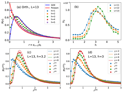
Figure 1: (a) The evolution of gap ratio distribution in an $L=13$ orthogonal system, $P(r)$ evolves from GOE to Poisson when the system is evolved from thermal ($h=1$) to MBL phase ($h=5$). (b) The evolution of inter-sample variance $V_{S}$ as a function of $h$, in systems with different sizes. Both the peak position and value of $V_{S}$ are larger in larger system, indicating a larger Giffiths regime. (c) $P\left(r^{(n)}\right)$ at the estimated transition point $h=3.2$ in an $L=13$ system, non-negligible deviations from SRPM are found due to residue correlations raised by finite-size effect. (d) $P\left(r^{(n)}\right)$ at $L=13$ and $h=3$, perfect matches with SRPM ($\beta=1$) are observed.

From the evolution of $P\left(r\right)$ in Fig. 1(a), we can have a qualitative estimation about the location of MBL transition point. To be specific, take a closer look at $P\left(r\right)$ at $h=3$ (the green dots in Fig. 1(a)), we see it lies roughly at the middle between GOE and Poisson, which indicates $h=3$ is close to the transition point.

To more quantitatively locate the transition point, we adopt a variant definition of gap ratio, which is

$$t_{i}=\frac{\min\left\{s_{i+1},s_{i}\right\}}{\max\left\{s_{i+1},s_{i}\right\}}$$ (10)

where $s_{i}=E_{i+1}-E_{i}$ is the $i$-th energy gap. This is actually the original definition of gap ratio introduced by Oganesyan and HuseOganesyan . Compared to $r_{i}$, $t_{i}$ takes values in the range $(0,1]$, and their distributions are related by $P\left(t\right)=2P\left(r\right)\Theta\left(1-r\right)$Atas . The mean value of gap ratio $\overline{t}$ can be easily calculated from Eq. (3), namely $\overline{t}_{\text{GOE}}=0.536$, $\overline{t}_{\text{GUE}}=0.603$ and $\overline{t}_{\text{Poisson}}=0.386$. Technically, the calculation of $\overline{t}$ has two steps: first we calculate the mean gap ratio value in one sample, which gives $t_{S}=\langle t_{i}\rangle_{\text{samp}}$, then we average $t_{S}$ over an ensemble of samples to get $\overline{t}=\langle r_{S}\rangle_{\text{en}}$. These two steps give two types of variance, the first one is $V_{S}=\langle t_{S}^{2}-\overline{t}^{2}\rangle_{\text{en}}$, i.e. the variance of sample-averaged gap ratio over ensemble, which measures the inter-sample randomness; another one is $V_{I}=\langle v_{I}\rangle_{\text{en}}$ where $v_{I}=\langle t_{i}^{2}-t_{S}^{2}\rangle_{\text{samp}}$, which is the ensemble-averaged gap ratio variance and measures the intrinsic intra-sample randomness. In a system driven by pure random disorder (that is, opposite to the ones induced by quasi-periodic potentialRD ), the distribution of $t_{S}$ near the transition region will exhibit strong deviation from a Gaussian type – a manifestation of Griffiths region – which results in a peak value of $V_{S}$ at the transition pointSierant19 . Therefore, for our model Eq. (1), we can calculate the evolution of $V_{S}$ to locate the transition point.

Strictly speaking, the transition point identified by $V_{S}$ and other quantities based on quantum entanglement may not always coincide in a finite system, meanwhile, $V_{S}$ in essence describes a qualitative structural change in the energy spectrum, hence is more suitable for our purpose to study the critical level statistics.

In Fig. 1(b) we draw the evolution of $V_{S}$ in systems with different lengths, where the number of samples are $10000,2000,500$ for $L=11,12,13$, respectively. In all cases, expected peaks of $V_{S}$ appear. We see that, in general, both the detected transition point and peak value $V_{S}$ are larger in larger system, which indicates a larger Griffiths regime, in consistence with the results in orthogonal model with $S_{Z}$ conservationSierant19 .

Now we are ready to count the level statistics at the transition region. In a finite system, what we observe is always a combination of universal part and non-universal (model dependent) part, we therefore choose the largest system we can reach to minimize the finite-size effects. That is, $L=13$ for systems without $S_{Z}$ conservation, and $L=16$ for those with $S_{Z}$ conservation. As for the present model with $L=13$, the detected transition point is, according to Fig. 1(b), $h_{c}\simeq 3.2\pm 0.2$.

First we take out the samples at the identified transition point $h=3.2$, and determine the corresponding gap ratio distributions $P\left(r^{\left(n\right)}\right)$ up to $n=4$, the results are displayed in Fig. 1(c), where the reference curves are the ones for SRPM in Eq. (9) with $\beta=1$. As we can see, the fittings have non-negligible deviations. We attribute this to the finite system size we are studying. That is, in a finite system, the eigenstates even in the MBL phase remain an exponentially decaying but finite correlations, hence the randomness required to drive the phase transition is slightly larger than it really needs in thermodynamic limit, which is in agreement with our analysis for Fig. 1(a). Therefore, the true critical level statistics is expected to occur in a point slightly smaller than $h=3.2$. To this end, we take out the samples from $h=3$ and count the corresponding $P\left(r^{\left(n\right)}\right)$, the results are in Fig. 1(d). As can be seen, they fit quite well with the SRPM, confirming the SRPM is indeed a good effective model, at least when level correlations on moderate ranges (up to $9$ levels) are concerned. To be complete, we have checked the same situations happen in the $L=12$ system.

To show this critical distribution is universal, we consider another orthogonal model, that is, the one with $h^{z}=h\neq 0,h^{x}=h^{y}=0$ in Eq. (1). This is actually the one most widely studied in the literature since it preserves total $S_{z}$, and allows one to reach to larger system size by focusing on one sector, which is commonly chosen to be the one with $S_{Z}^{T}=0$. Technically, this also requires the number of spins $L$ to be even. However, eigenstates in this sector share one common feature, i.e. $S_{Z}^{T}=0$, which violates the featureless property of a fully thermalized state. Therefore, the eigenstates in this sector is easier to be localized, which results in a large large finite-size effect, and the estimated transition point is much less smaller than the interpolated value in thermodynamic limit. Actually, it’s widely accepted the transition point is around $h_{c}\simeq 3.6$ for the middle part of energy spectrum, while in a finite system, say $L=16$, the detected transition point is shifted to $h_{c}\simeq 2.7$Sierant19 .

In our study, we take the system size to be $L=16$ and focus on the $S_{Z}^{T}=0$ sector, whose Hilbert space’s dimension is $N=C_{16}^{8}=\frac{16!}{8!8!}=12870$. Like before, we first present a qualitative picture for the gap ratio’s evolution in the range $h\in\left[1,5\right]$, with $500$ samples taken at each point, the results are displayed in Fig. 2(a), we see a GOE-Poisson evolution as expected. Then we numerically determine the evolution of inter-sample randomness $V_{S}$, which is presented in Fig. 2(b). The observed peak indicates a transition at $h=2.6\pm 0.2$, in well accordance with the previous studies in this system size. Next we consider the critical statistics. With the same reason as for previous model, we take the samples from $h=2.4$, slightly smaller than the estimated one, and the corresponding $P\left(r^{\left(n\right)}\right)$ are displayed in Fig. 2(c). As can be seen, they fit quite good with the prediction of SRPM with $\beta=1$.

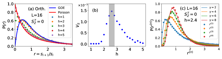
Figure 2: (a) The evolution of gap ratio distribution $P(r)$ in the $S_{Z}^{T}=0$ sector of the $L=16$ orthogonal model, an expected GOE-Poisson transition is found. (b) The evolution of $V_{S}$, which indicates the transition point is $h_{c}=2.6\pm 0.2$. (c) $P\left(r^{(n)}\right)$ at $h=2.4$, a perfect match with SRPM ($\beta=1$) is observed, indicating this effective model is universal.

Up to now, we have confirmed the SRPM with $k=\beta=1$ is a quite good effective model for the critical spectral statistics in an orthogonal model, not only for nearest-neighbor gap ratios, but also for several higher-order ones that describe level correlations on longer ranges, and this model is expected to be universal that independent of microscopic details. In the next section, we will proceed to study the unitary model.

IV Unitary Models

Now we study the critical level statistics in unitary models, we will show it is well described by SRPM with $k=1$ and $\beta=2$. Like before, we first consider the case without $S_{Z}^{T}$ conservation, that is, the model Eq. (1) with $h_{x}=h_{y}=h_{z}=h\neq 0$. Likewise, we work on an $L=13$ system, the qualitative evolution of $P\left(r\right)$ is given in Fig. 3(a), a GUE-Poisson evolution is observed when increasing randomness as expected. From the evolution, we can qualitatively see the transition point lies at somewhere between $h=2$ and $h=3$. Next, we calculate the evolution of inter-sample randomness $V_{S}$, the result is given in Fig. 3(b). We see an expected peak indicating the transition point is $h_{c}\simeq 2.8\pm 0.2$, close to $h_{c}\simeq 2.5$ got by previous studiesRegnault16 ; Regnault162 .

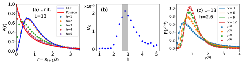
Figure 3: (a) The evolution of $P(r)$ in an $L=13$ unitary system, a GUE-Poisson transition is observed as expected. (b) The evolution of inter-sample randomness $V_{S}$, and the shaded area indicates the transition region $h_{c}=2.8\pm 0.2$. (c) $P\left(r^{(n)}\right)$ at $h=2.6$, a good match with SRPM ($\beta=2$) is observed.

Next, we are considering the critical level statistics. With the same reason as in previous section, we take a point slightly left to the estimated one, that is $h=2.6$, and the corresponding $P\left(r^{\left(n\right)}\right)$ are presented in Fig. 3(c). As can been seen, they fit very well with the predictions of SRPM with $k=1$ and $\beta=2$, which provides a strong evidence that the SRPM is a good effective model.

To further show this critical behavior in the unitary model is also universal, we study a unitary spin model with total $S_{Z}$ conservation, which is constructed by adding a time-reversal breaking next-nearest neighboring interaction term to the Heisenberg model, the Hamiltonian then reads

$$H=\sum_{i=1}^{L}\left[\mathbf{S}_{i}\cdot\mathbf{S}_{i+1}+J\mathbf{S}_{i}\cdot\left(\mathbf{S}_{i+1}\times\mathbf{S}_{i+2}\right)\right]+h\sum_{i=1}^{L}\varepsilon_{i}^{z}S_{i}^{z}\text{.}$$ (11)

This model was introduced to generate the GUE statistics in Ref. [Avishai2002, ], it was also pointed out the level statistics almost immediately changes from GOE to GUE even when $J$ is as small as $0.01$Avishai2002 . The thermal-MBL transition point in this model certainly depends on $J$: in general, the larger $J$, the larger $h_{c}$ will be. In this work, we choose $J=0.2$ without loss of generality, and focusing on the $S_{Z}^{T}=0$ sector in an $L=16$ system.

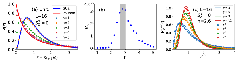
Figure 4: (a) The evolution of $P(r)$ in the $S_{Z}^{T}=0$ sector of the $L=16$ unitary model with the next-nearest neighboring interaction strength $J=0.2$, an expected GUE-Poisson transition is found. (b) The evolution of $V_{S}$, which indicates the transition region is $h_{c}=2.8\pm 0.2$. (c) $P\left(r^{(n)}\right)$ at $h=2.6$, minor deviations from SRPM with $\beta=2$ are observed, which may be attributed to the large finite-size effect induced by the next-nearest neighboring interaction that destroys the integrability of pure Hamiltonian. The dotted lines: SRPM with $\beta=1.7$.

The qualitative evolution of $P\left(r\right)$ is given in Fig. 4(a), a GUE-Poisson evolution when increasing randomness $h$ is observed as expected. Next, we calculate the evolution of inter-sample randomness $V_{S}$, the result is presented in Fig. 4(b). We see an expected peak indicating the transition point is $h_{c}\simeq 2.8\pm 0.2$. Interestingly, this coincides with the one in Fig. 3(b), which is purely accidental for the $J=0.2$ we choose. Actually, the values of $V_{S}$ in Fig. 4(b) are much larger than those in Fig. 3(b), which means the inter-sample randomness is generally larger in this model, hence the finite-size effect is expected to be more serious.

Next, we are considering the critical statistics. Like before, we take a point slightly smaller than the estimated one, that is $h=2.6$, and the corresponding $P\left(r^{\left(n\right)}\right)$ are presented in Fig. 4(c). As can been seen, they qualitatively meets the predictions of SRPM with $k=1$ and $\beta=2$, but the deviations are larger than those in Fig. 3(c). We attribute this to the next-nearest interaction term that destroys the integrability of the pure model, which strengthens the thermal phase in the random model and results in a more serious finite-size effect, in accordance with our analysis about Fig. 4(b). In fact, if we artificially allow the inverse temperature to be a fraction, we find the $P\left(r^{\left(n\right)}\right)$ in Fig. 4(c) can be well fitted into $\beta=1.7$ (the dotted lines in Fig. 4(c)), which is close to the expected value $\beta=2$.

To conclude, we have shown the spectral statistics in the transition region of a unitary model without $S_{Z}^{T}$ conservation is well described by the SRPM with $k=1$ and $\beta=2$, which is a natural extension of the one for the orthogonal system. The results from unitary model with $S_{Z}^{T}$ conservation suggests this critical behavior is also universal for unitary model, although the deviations are slightly larger. We suggest a future work on larger system to confirm this conclusion.

V Conclusion and Discussion

We have studied the thermal-MBL transition in both orthogonal and unitary models in random spin systems. By using the inter-sample randomness as the “order parameter”, we successfully located the transition points, which are in well agreement with previous studies. We then determine the $n$-th order gap ratio distributions up to $n=4$ at the critical region, and confirm they fit well with the short-range plasma model (SPRM) with inverse temperature $\beta=1$ for orthogonal model and $\beta=2$ for unitary. Based on results from models both with and without $S_{Z}^{T}$ conservation, we argue these critical behaviors are universal that independent of microscopic details.

It is worth noting that the level statistics right at the transition points detected by $V_{S}$ show systematic deviations from SRPM in all cases studied, this is due to the finite size effect. To be precise, in a finite system, there will always remain exponentially decaying but finite level correlations even deep in the MBL phase, as can be seen from the fitting results for MBL phases in Fig.1(a),2(a),3(a) and 4(a). Therefore, the randomness strength to drive the phase transition will be larger to compensate for these residue level correlations. Consequently, the true critical statistics will appear slightly left to the detected transition point. The deviations in the unitary model with $S_{Z}^{T}$ conservation are larger than the rest models, which can be attributed to the neat-nearest neighboring interactions. That is, the next-nearest neighboring term breaks the integrability of the clean system and stabilizes the thermal phase in disordered system, which results in larger residue level correlations in a finite system. After all, in all cases, what we observe is a combination of universal critical level statistics and non-universal (model-dependent) finite-size results, for which a detailed quantification will require a systematic finite-size scaling study, and is left for a future work.

It would be beneficial to compare the SRPM with other proposed effective models for the transition region, first of which is the mean-field plasma model (MFPM), which is proposed by Serbyn and Moore by mapping the thermal-MBL transition into a random walk process in the Hilbert spaceSerbyn . Mathematically, both SRPM and MFPM describe the energy levels of a random matrix ensemble as an ensemble of 1D classical particles, however in SRPM the interaction form stays unchanged and interaction range is responsible for the thermal-MBL transition, while the inverse is true for the MFPM. Meanwhile, both models hold the semi-Poisson distribution for the nearest level spacings, hence our results are not controversial to those in Ref. [Serbyn, ]. In this study, we proceed to consider the higher-order level correlations, and find good support for the SRPM. In fact, our results suggest the form of local interaction between energy levels stays logarithmic during the phase transition, and the change in interaction range can be revealed by the high-order level correlations. Another proposed effective model is the Gaussian $\beta$ ensemble, which has the same structure as the GOE,GUE,GSE but the Dyson index $\beta$ takes value in $\left(0,\infty\right)$. In Ref. [Buijsman, ] the authors showed the Gaussian ensemble with non-integer $\beta$ can describe the lowest-order gap ratio distribution across the thermal-MBL transition quite well but the fittings for higher-order ones have large deviations. This also suggests the form of interaction between levels stays logarithmic but the interaction range changes during phase transition, hence is also consistent with our results.

Another interesting fact to notice is that the SRPM can emerge from the Poisson ensemble, that is, the SRPM with $k=1$ and inverse temperature $\beta$ has the same structure as the $\beta$-th order reduced energy spectrum of a Poisson ensembleDaisy (which is called “Daisy model” by the authors). This indicates the universal lower-order spectral statistics at the transition region are secretly hidden in the eigenvalue spectrum of the MBL phase, for which a full physical understanding is lacking by now. However, this at least indicates the thermal-MBL transition point is more affected by the MBL phase rather than the thermal phase, a fact that has already been noticed by previous studies based on eigenfunction propertiesHuse2 ; Serbyn ; Sierant19 and now appears again by means of the reduced energy spectrum. On the other hand, in Ref. [Daisy, ] the authors declare the absence of a dynamical system that corresponds to the “Daisy model” with inverse temperature $\beta>1$, our work thus suggests the thermal-MBL transition point in unitary system is a natural candidate for $\beta=2$.

Last but not least, the SRPM was debated for its effectiveness in describing long range level correlations at the MBL transitionSierant19 , e.g. through the number variance $\Sigma^{2}$. Unfortunately our attempts to fit $\Sigma^{2}$ do not give conclusive results. This may partially due to the intrinsic sensitive dependence of $\Sigma^{2}$ on concrete unfolding procedureGomez2002 , and also may results from the limited system size we can reach. Nevertheless, our results support the SRPM is a good effective model not only for lowest-order level correlations, but also for correlations on moderate longer ranges. We left an improved study on larger system size for a future work.

References

- (1) I. V. Gornyi, A. D. Mirlin, and D. G. Polyakov, Phys. Rev. Lett. 95, 206603 (2005); 95, 046404 (2005).
- (2) D. M. Basko, I. L. Aleiner, and B. L. Altshuler, Ann. Phys. 321, 1126 (2006).
- (3) J. A. Kjall, J. H. Bardarson, and F. Pollmann, Phys. Rev. Lett. 113, 107204 (2014).
- (4) S. D. Geraedts, N. Regnault, and R. M. Nandkishore, New J. Phys. 19, 113921 (2017).
- (5) Z. C. Yang, C. Chamon, A. Hamma, and E. R. Mucciolo, Phys. Rev. Lett. 115, 267206 (2015).
- (6) M. Serbyn, A. A. Michailidis, M. A. Abanin, and Z. Papic, Phys. Rev. Lett. 117, 160601 (2016).
- (7) J. Gray, S. Bose, and A. Bayat, Phys. Rev. B 97, 201105 (2018).
- (8) M. Serbyn, Z. Papic, and D. A. Abanin, Phys. Rev. X 5, 041047 (2015).
- (9) H. Kim and D. A. Huse, Phys. Rev. Lett. 111, 127205 (2013).
- (10) J. H. Bardarson, F. Pollman, and J. E. Moore, Phys. Rev. Lett. 109, 017202 (2012).
- (11) M. Serbyn, Z. Papić, and D. A. Abanin, Phys. Rev. B 90, 174302 (2014).
- (12) M. L. Mehta, Random Matrix Theory, Springer, New York (1990).
- (13) F. Haake, Quantum Signatures of Chaos, (Springer 2001).
- (14) V. Oganesyan and D. A. Huse, Phys. Rev. B 75, 155111 (2007).
- (15) Y. Avishai, J. Richert, and R. Berkovits, Phys. Rev. B 66, 052416 (2002).
- (16) N. Regnault and R. Nandkishore, Phys. Rev. B 93, 104203 (2016).
- (17) S. D. Geraedts, R. Nandkishore, and N. Regnault, Phys. Rev. B 93, 174202 (2016).
- (18) V. Oganesyan, A. Pal, D. A. Huse, Phys. Rev. B 80, 115104 (2009).
- (19) A. Pal, D. A. Huse, Phys. Rev. B 82, 174411 (2010).
- (20) S. Iyer, V. Oganesyan, G. Refael, D. A. Huse, Phys. Rev. B 87, 134202 (2013).
- (21) D. J. Luitz, N. Laflorencie, and F. Alet, Phys. Rev. B 91, 081103(R) (2015).
- (22) K. Agarwal, S. Gopalakrishnan, M. Knap, M. Múller, and Eugene Demler, Phys. Rev. Lett. 114, 160401 (2015).
- (23) S. Gopalakrishnan, K. Agarwal, E. Demler, D. A. Huse, and M. Knap, Phys. Rev. B 93, 134206 (2016).
- (24) K. Agarwal, E. Altman, E. Demler, S. Gopalakrishnan, D. A. Huse, and M. Knap, Ann. Phys. 1600326 (2017).
- (25) D. J. Luitz and Y. Bar Lev, Ann. Phys. 529 (7), 1600350 (2017).
- (26) F. Alet and N. Laflorencie, C. R. Physique 19, 498-525 (2018).
- (27) N. Macé, F. Alet, and N. Laflorencie, Phys. Rev. Lett. 123, 180601 (2019).
- (28) P. Shukla, New Journal of Physics 18, 021004 (2016).
- (29) M. Serbyn and J. E. Moore, Phys. Rev. B 93, 041424(R) (2016).
- (30) E. B. Bogomolny, U. Gerland and C. Schmit, Eur. Phys. J. B 19, 121 (2001).
- (31) P. Sierant and J. Zakrzewski, Phys. Rev. B 99, 104205 (2019).
- (32) W. Buijsman, V. Cheianov and V. Gritsev, Phys. Rev. Lett. 122, 180601 (2019).
- (33) P. Sierant and J. Zakrzewski, Phys. Rev. B 101, 104201 (2020).
- (34) M. L. Ndawana and V. E. Kravtsov, J. Phys. A 36, 3639 (2003).
- (35) S. Ray, B. Mukherjee, S. Sinha, and K. Sengupta, Phys. Rev. A 96, 023607 (2017).
- (36) B. I. Shklovskii, B. Shapiro, B. R. Sears, P. Lambrianides, and H. B. Shore, Phys. Rev. B 47 11487 (1993).
- (37) J. M. G. Gomez, R. A. Molina, A. Relano, and J. Retamosa, Phys. Rev. E 66, 036209 (2002).
- (38) Y. Y. Atas, E. Bogomolny, O. Giraud, and G. Roux, Phys. Rev. Lett. 110, 084101 (2013).
- (39) S. H. Tekur, U. T. Bhosale, and M. S. Santhanam, Phys. Rev. B 98, 104305 (2018).
- (40) W.-J. Rao, Phys. Rev. B 102, 054202 (2020).
- (41) W.-J. Rao and M. N. Chen, Eur. Phys. J. Plus 136, 81 (2021).
- (42) Y. Y. Atas, E. Bogomolny, O. Giraud, P. Vivo, and E. Vivo, J. Phys. A: Math. Theor. 46, 355204 (2013).
- (43) H. Hernández-Saldaña, J. Flores, and T. H. Seligman, Phys. Rev. E 60, 449 (1999).
- (44) V. Khemani, D. N. Sheng, and D. A. Huse, Phys. Rev. Lett. 119, 075702 (2017).