Aharonov-Bohm effect in three-dimensional higher-order topological insulators

Abstract

The 1D hinge states are the hallmark of the 3D higher-order topological insulators (HOTI), which may lead to interesting transport properties. Here, we study the Aharonov-Bohm (AB) effect in the interferometer constructed by the hinge states in the normal metal-HOTI junctions with a transverse magnetic field. We show that the AB oscillation of the conductance can clearly manifest the spatial configurations of such hinge states. The magnetic fluxes encircled by various interfering loops are composed of two basic ones, so that the oscillation of the conductance by varying the magnetic field contains different frequency components universally related to each other. Specifically, the four dominant frequencies $\omega_{x,y}$ and $\omega_{x\pm y}$ satisfy the relations $\omega_{x\pm y}=\omega_{x}\pm\omega_{y}$, which generally holds for different magnetic field, sample size, bias voltage and weak disorder. Our results provide a unique and robust signature of the hinge states and pave the way for exploring AB effect in the 3D HOTI.

I INTRODUCTION

Over the past two decades, topological phases of matter such as topological insulator and superconductor have become an active research field of condensed matter physics Qi and Zhang (2011); Hasan and Kane (2010). These materials are characterized by the nontrivial band topology and the resultant gapless (d-1)-dimensional edge states. Very recently, the concepts of higher-order topological insulators (HOTI) and superconductors are theoretically proposed, which are featured by the $(d-2)$-dimensional edge states Benalcazar et al. (2017a, b); Song et al. (2017); Langbehn et al. (2017); Schindler et al. (2018a); Franca et al. (2018); Park et al. (2019); Khalaf (2018); Vu et al. (2020); Zhang et al. (2020); Yan (2019a); Călugăru et al. (2019); Yan (2019b); Yan et al. (2018); Schindler et al. (2018b). Specifically, for the 3D HOTI there exist 1D gapless states along the hinges of the sample, so-called hinge states, while the surface and the bulk states are both insulating. Recent progresses have shown the evidences of the hinge states in bismuth by the scanning-tunnelling spectroscopy and Josephson interferometry Schindler et al. (2018b), which pave the way for exploring more intriguing properties of such topological states in the HOTI.

The 1D nature of the hinge states indicates that it is a good playground for exploring various interference effects, such as Aharonov-Bohm (AB) and Fabry-Pérot interferometers Liang et al. (2001); van Wees et al. (1989); Ji et al. (2003); Ofek et al. (2010); McClure et al. (2009); Nakamura et al. (2019). Actually, the chiral edge states of the quantum Hall phase have become an important platform for the study of mesoscopic physics, in which a variety of novel phenomena have been observed Ji et al. (2003); Henny et al. (1999); Neder et al. (2007); Weisz et al. (2014) due to its long coherence length and high adjustability. Compared with the chiral edge states, the hinge states in the HOTI open additional possibilities for the implementation of novel effects due to their 3D configurations, which enrich the way of interfering in real space. Moreover, such effects cannot be realized in any 2D systems, which in turn, can serve as the deterministic evidence of the hinge states.

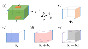
Figure 1: (a) The interferometer constructed by HOTI (green block) and normal metal electrodes (orange blocks). The magnetic field $B$ is imposed in $x$-$y$ plane with a polar angle $\theta$. (b, c) Two elemental interfering loops with encircled flux $\Phi_{x}$, $\Phi_{y}$. (d, e) Other two dominant interfering loops with fluxes $\Phi_{x}+\Phi_{y}$, $|\Phi_{x}-\Phi_{y}|$.

The manifestation of the AB effect in an electron system is the periodic oscillation of conductance as the closed trajectory of electrons encircles a magnetic flux $\Phi$ Aharonov and Bohm (1959); Webb et al. (1985); Holloway et al. (2015); Lahiri et al. (2018); Aleiner et al. (2015); Tserkovnyak and Halperin (2006). The dominant period of oscillation is equal to the flux quantum $\Phi_{0}=h/e$, with a main frequency $2\pi/\Phi_{0}$. The frequency of oscillation can be found by taking the fast Fourier transform (FFT) of the conductance pattern Webb et al. (1985); Holloway et al. (2015); Lahiri et al. (2018). Recently, AB effect has been used as an effective way to detect edge states in various topological systems, such as edge states of topological insulators Peng et al. (2010); Bardarson et al. (2010); Zhang and Vishwanath (2010); Xypakis et al. (2020), Majorana fermions of topological superconductors Li et al. (2012); Ueda and Yokoyama (2014); Tripathi et al. (2016); Bartolo et al. (2020), surface states of topological semimetal Wang et al. (2016); Lin et al. (2017), and non-Abelian anyons of fractional quantum Hall systems Kim (2006); Halperin et al. (2011); Willett et al. (2013); Nakamura et al. (2019, 2020).

In this work, we investigate the AB effect in the interferometer composed of the hinge states of the quadrangular HOTI by imposing an external magnetic field. The insulating bulk and surface states indicate that the electron can only propagate along the hinges of the sample, by which the enclosed magnetic flux can lead to a coherent oscillation of the transmission probability. Different from the edge states in any 2D systems, the 3D network of the hinge states results in peculiar interfering trajectories, which relies not only on the magnitude of the magnetic field but also on its orientation. The AB interferometer is sketched in Fig. 1(a), where the HOTI is connected to two leads made of the normal metal and a magnetic field $\bm{B}=(B_{x},B_{y})=B(\cos\theta,\sin\theta)$ is applied in the $x$-$y$ plane with $\theta$ being the polar angle. The electrons injected from the leads propagate along four chiral hinge states, which comprise a variety of interfering loops; see Figs. 1(b)-1(e). The elemental interfering loops shown in Figs. 1(b) and 1(c) are exactly the boundaries of the ($\pm$1,0,0) and (0,$\pm$1,0) surfaces. The basic loops in Figs. 1(b) and 1(c) encircle a magnetic flux of $\Phi_{x}=B\cos\theta S_{x}$ and $\Phi_{y}=B\sin\theta S_{y}$, respectively, with $S_{x,y}$ the surface areas. Accordingly, the frequency components $\omega_{x}=2\pi\cos\theta S_{x}/\Phi_{0}$ and $\omega_{y}=2\pi\sin\theta S_{y}/\Phi_{0}$ naturally appear in the oscillating pattern of the conductance as the magnetic field $B$ varies. Interestingly, the magnetic flux in other interfering loops can all be interpreted by the two elemental ones, among which two typical loops in Figs. 1(d) and 1(e) contain a flux of $\Phi_{x\pm y}=\Phi_{x}\pm\Phi_{y}$, and the corresponding oscillating frequency components satisfy $\omega_{x\pm y}=\omega_{x}\pm\omega_{y}$. It turns out that the aforementioned four interfering loops and the corresponding oscillating frequencies dominant the coherent oscillation of the conductance. The relation $\omega_{x\pm y}=\omega_{x}\pm\omega_{y}$ generally holds independent of various parameters such as the magnetic field, sample size and the energy of electron, thus providing a universal and deterministic signature of the hinge states and HOTI.

The rest of this paper is organized as follows. In Sec. II, we elucidate the model of the HOTI adopted in our work. In Sec. III, we apply the scattering matrix approach to analyze the coherent transport through the interferometer and the AB oscillation of the conductance. Detailed numerical simulations on the lattice model are conducted in Sec. IV, which verify the universality of the physical results. Finally, a brief summary and outlook are given in Sec. V.

II Model of HOTI

We adopt the model of 3D chiral HOTI introduced by Schindler et al. Schindler et al. (2018a) as

$$\begin{split}H_{\text{HOTI}}&=\left(M+t\sum_{i}{\cos k_{i}}\right)\tau_{z}\sigma_{0}+\Delta_{1}\sum_{i}{\sin k_{i}\tau_{x}\sigma_{i}}\\ &\ \ \ +\Delta_{2}(\cos k_{x}-\cos k_{y})\tau_{y}\sigma_{0},\end{split}$$ (1)

where $\sigma_{i=x,y,z}$ and $\tau_{i}$ are the Pauli matrices acting on the spin and orbital space, respectively. For $1<|M/t|<3$ and $\Delta_{1},\Delta_{2}\neq 0$, the system lies in a chiral 3D HOTI phase. The energy spectra are gapped in both the bulk and four surfaces parallel to the $z$-axis. Importantly, the mass term is opposite in sign between adjacent surfaces that results in the Jackiw-Rebbi-type bound states Jackiw and Rebbi (1976) propagating only along the $\pm z$-direction, or the so-called topological hinge states. Time-reversal symmetry is broken in Eq. (1), so that the hinge states are unidirectional or chiral, without any backscattering states within a given hinge. Notably, gapless Dirac cones protected by the $\hat{C}_{4}^{z}\hat{T}$ symmetry persist on the surfaces perpendicular to the $z$-axis Schindler et al. (2018a). Therefore, it is beneficial to explore pure signature of the hinge states through the transport in the $z$-direction.

III Scattering matrix analysis

In this section, we study the coherent transport of electrons through the interferometer sketched in Fig. 1(a) based on the low-energy effective model of the hinge states using the scattering matrix approach. The scattering matrix of the whole interferometer can be obtained by combining those at two normal metal-HOTI interfaces and the matrix of phase accumulation during propagation in the hinge states. The matrix at the lower interface [cf. Fig. 1(a)] can be parameterized as

$$S_{l}=\left(\begin{array}[]{cccc}r_{1}&r_{3}&t_{1}^{\prime}&t_{3}^{\prime}\\ r_{2}&r_{4}&t_{2}^{\prime}&t_{4}^{\prime}\\ t_{1}&t_{3}&r_{1}^{\prime}&r_{3}^{\prime}\\ t_{2}&t_{4}&r_{2}^{\prime}&r_{4}^{\prime}\\ \end{array}\right),$$ (2)

which relates the incoming ($a_{l}$) and outgoing ($b_{l}$) waves in the normal metal and the HOTI via $b_{l}=S_{l}a_{l}$. The matrix is assumed to be $4\times 4$ such that two incoming/outgoing waves are taken into account on both sides. For the HOTI, the number of channels corresponds to that of pairs of the hinge states. The unitary condition $S_{l}S_{l}^{\dagger}=\text{I}$ is ensured by the law of current conservation. Here, $t_{1,\cdots,4}$ are the transmission amplitudes from the normal metal to the chiral hinge states of the HOTI and $r_{1,\cdots,4}$ are the corresponding reflection amplitudes. The scattering amplitudes corresponding to the incident waves from the hinge states of HOTI are defined by $t^{\prime}_{1,\cdots,4},r^{\prime}_{1,\cdots,4}$ in a similar way. The scattering matrix for the upper interface can be defined as

$$S_{u}=\left(\begin{array}[]{cccc}r_{1}^{u}&r_{3}^{u}&t_{1}^{u\prime}&t_{3}^{u\prime}\\ r_{2}^{u}&r_{4}^{u}&t_{2}^{u\prime}&t_{4}^{u\prime}\\ t_{1}^{u}&t_{3}^{u}&r_{1}^{u\prime}&r_{3}^{u\prime}\\ t_{2}^{u}&t_{4}^{u}&r_{2}^{u\prime}&r_{4}^{u\prime}\\ \end{array}\right).$$ (3)

The phase modulation of the wave function due to the magnetic field can be described by the matrix as

$$S_{m}=\left(\begin{array}[]{cccc}0&0&e^{i\tilde{\phi_{1}}}&0\\ 0&0&0&e^{-i\tilde{\phi_{2}}}\\ e^{-i\phi_{2}}&0&0&0\\ 0&e^{i\phi_{1}}&0&0\\ \end{array}\right)$$ (4)

where the phases $\phi_{1},\phi_{2},\tilde{\phi_{1}},\tilde{\phi_{2}}$ are related by the magnetic fluxes through $\phi_{1}+\tilde{\phi_{1}}=\phi_{2}+\tilde{\phi_{2}}=\phi_{x}=2\pi\Phi_{x}/\Phi_{0},\phi_{1}-\tilde{\phi_{2}}=\phi_{2}-\tilde{\phi_{1}}=\phi_{y}=2\pi\Phi_{y}/\Phi_{0},\phi_{1}+\phi_{2}=\phi_{x+y}=2\pi\Phi_{x+y}/\Phi_{0}$ and $\tilde{\phi_{1}}+\tilde{\phi_{2}}=\phi_{x-y}=2\pi\Phi_{x-y}/\Phi_{0}$ with $\phi_{x,y}$ and $\phi_{x\pm y}$ being gauge invariant.

By combining three matrices $S_{l},S_{m},S_{u}$ in a standard way we obtain the total scattering matrix for the whole system. Here, we focus on the periods of the AB oscillation and an overall phase shift of the pattern is unimportant. Therefore, we can choose $S_{l},S_{u}$ to be real for simplicity which will not change the main results. For an electron incident from the lower terminal, its transmission probability $T$ to upper terminal is obtained after some algebra as

$$\begin{split}T&=F^{-1}\Big{[}C+C_{X}\cos\phi_{x}+C_{Y}\cos\phi_{y}+C_{XY}\cos\phi_{x+y}+C_{XY}^{\prime}\cos\phi_{x-y}\Big{]},\\ F&=M_{C}+M_{XY}\cos\phi_{x+y}+M_{XY}^{\prime}\cos\phi_{x-y}+M_{2X}\cos(2\phi_{x})+M_{2Y}\cos(2\phi_{y})-M_{X}\cos\phi_{x}-M_{Y}\cos\phi_{y},\end{split}$$ (5)

where the explicit forms of the relevant parameters are given in Appendix A. The numerator of the transmission in Eq. (5) shows that there are four dominant periodic terms contributed by four interference loops in Figs. 1(b)-1(e) which correspond to four frequencies related by $\omega_{x,y},\omega_{x\pm y}=\omega_{x}\pm\omega_{y}$. Note that such relations are stabilized by the spatial configurations of the hinge states, thus offer a clear and robust signature for its detection, which relies little on the sample details and the energy. Although magnetic field in different directions will change the values of frequencies it does not affect the general relations between them.

Next, we provide numerical verification of such an observation using specific scattering amplitudes. The AB oscillation of the conductance as a function of $B$ and its FFT spectrum are shown in Figs. 2(a) and 2(b), respectively. The polar angle of the magnetic field is set to $\theta=\pi/6$ and the unit of frequency is chosen as $1/B_{0}$ with $B_{0}=\Phi_{0}/(2\pi S)$ and $S=S_{x}=S_{y}$ the surface area. One can find multiple periods in the conductance spectrum in Fig. 2(a). The FFT spectrum in Fig. 2(b) shows that there are four dominant frequencies with $\omega_{x}=0.86/B_{0},\omega_{y}=0.5/B_{0},\omega_{x-y}=0.36/B_{0},\omega_{x+y}=1.36/B_{0}$, which conforms the aforementioned relation $\omega_{x\pm y}=\omega_{x}\pm\omega_{y}$. Higher frequencies such as $\omega_{2x},\omega_{2y}$ should also appear as that in the conventional 2D AB effect. In stark contrast, the frequencies $\omega_{x\pm y}$ can only exist in the 3D HOTI, which thus provides a unique evidence of the hinge states.

Figure 2: (a) The conductance pattern calculated by the scattering matrices. (b) The FFT spectrum of the oscillation pattern. The relevant scattering coefficients are set to $t_{1}=t_{3}=t_{4}=r_{1}^{\prime}=r_{1}^{u}=r_{2}^{u}=\sqrt{0.4},t_{2}=r_{3}^{\prime}=\sqrt{0.3},r_{1}=r_{2}^{\prime}=\sqrt{0.2},r_{2}=r_{3}=r_{4}=t_{1}^{u}=t_{2}^{u}=t_{3}^{u}=\sqrt{0.1},r_{4}^{\prime}=t_{4}^{u}=-\sqrt{0.1},r_{3}^{u}=r_{4}^{u}=-\sqrt{0.4}.$

IV Lattice model simulation

Based on the scattering matrix analysis, we see that there are four dominant frequencies satisfying universal relations $\omega_{x\pm y}=\omega_{x}\pm\omega_{y}$. In this section, we perform numerical simulation to give rigorous results. We write the model in Eq. (1) on a cubic lattice as Levitan and Pereg-Barnea (2020)

$$H^{\text{Lattice}}_{\text{HOTI}} =\sum_{i}{c_{i}^{\dagger}M\sigma_{0}\tau_{z}c_{i}}$$ (6)

$$+\Bigg{\{}\sum_{i}{{c_{i+x}^{\dagger}\bigg{[}\frac{e^{i\varphi_{x}}}{2}(\Delta_{2}\sigma_{0}\tau_{y}+t\sigma_{0}\tau_{z}+i\Delta_{1}\sigma_{x}\tau_{x})\bigg{]}c_{i}}}$$

$$-\sum_{i}{c_{i+y}^{\dagger}(\Delta_{2}\sigma_{0}\tau_{y}+t\sigma_{0}\tau_{z}+i\Delta_{1}\sigma_{y}\tau_{x})c_{i}}$$

$$+\sum_{i}{c_{i+z}^{\dagger}\frac{e^{i\varphi_{z}}}{2}(t\sigma_{0}\tau_{z}+i\Delta_{1}\sigma_{z}\tau_{x})c_{i}}+h.c.\Bigg{\}},$$

where $c_{i}=(c_{a,\uparrow,i},c_{b,\uparrow,i},c_{a,\downarrow,i},c_{b,\downarrow,i})$ are the annihilate operators at lattice site $i$ with two spin ($\uparrow,\downarrow$) and two orbit ($a,b$) components. The Peierls phase $\varphi_{x,z}=\frac{e}{\hbar}\int_{r_{i}}^{r_{j}}\bm{A}(\bm{r})\cdot d\bm{r}$, where $\bm{A}(\bm{r})=(B_{y}z,0,B_{x}y)$ is the vector potential under Landau gauge. The lattice model of the normal metal electrodes is

$$H_{\text{NM}} =\sum_{i}{(-6t+U)c_{i}^{\dagger}c_{i}}$$ (7)

$$+\sum_{i}{t(c_{i+x}^{\dagger}c_{i}+c_{i+y}^{\dagger}c_{i}+c_{i+z}^{\dagger}c_{i})}+h.c..$$

Figure 3: (a) Conductance oscillation for different incident energy and angle $\theta$ by the lattice simulation. An offset $2e^{2}/h$ is imposed to adjacent curves for clarity. (b, c) Corresponding FFT spectra of the conductance patterns. Four dominant frequencies are marked by the dashed lines. The model parameters are set to $t=-1,M=2.3,\Delta_{1}=0.8,\Delta_{2}=0.5,U=2$. The lattice of the HOTI is set to a $30a\times 30a\times 30a$ cube, where $a=1$ is the lattice constant.

The AB interferometer constructed by the 3D HOTI (green block) and the normal metal leads (two orange blocks) is shown in Fig. 1(a). The blue arrowed lines denote the chiral hinge states. The cross section of the HOTI in the $x$-$y$ plane is set as $30a\times 30a$ and that for the normal metal leads is $5a\times 5a$ with $a$ being the lattice constant. The magnetic field $B$ exists only in the HOTI region and is parallel to the $x$-$y$ plane.

Consider an electron impinging from the normal metal towards the HOTI with its energy lying in the bulk gap ($\simeq$0.7$|t|$) and surface gap ($\simeq$0.32$|t|$) of the HOTI, so that only the hinge channels are available for propagation. Backscattering can occur at the interfaces, giving rise to various interference loops. The two terminal conductance $G$ is calculated using KWANT package Groth et al. (2014) and the AB conductance oscillation for different incident energy ($ie$) and polar angle $\theta$ of magnetic field are shown in Fig. 3(a) (curves are offset by $2e^{2}/h$ for clarity). To get the dominant frequencies, we perform FFT calculation whose spectra are shown in Figs. 3(b) and 3(c).

The numerical results are consistent with those by the scattering matrix analysis in Figs. 2(b). For different incident energies, the oscillation patterns in Fig. 3(a) look in stark difference. However, the dominant frequencies remain almost the same; see Fig. 3(b). To check the general relations between oscillation frequencies, we first locate two notable peaks $\omega_{x}$ and $\omega_{y}$ by the dashed lines and the other two peaks $\omega_{x\pm y}=\omega_{x}\pm\omega_{y}$ are marked accordingly in Fig. 3(b). One can see that the dominant peaks match the dashed lines very well apart from a small deviation from $\omega_{x+y}$ for $ie=0.1$ which is attributed to the limit of numerical calculations. For different polar angle $\theta$, similar results can be seen in Fig. 3(c). Although the location of peaks change for different $\theta$, the general relations between them persist.

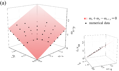
Figure 4: (a) $\omega_{x+y}$ and (b) $\omega_{x-y}$ as a function of elemental frequencies $\omega_{x}$ and $\omega_{y}$. Black and orange dots denote numerical results for different length of the HOTI and polar angle $\theta$ of the magnetic field. The reference planes satisfy $\omega_{x\pm y}=\omega_{x}\pm\omega_{y}$. Insets: side view of the plots which reveal the deviation of the dots from the planes. The parameters are the same as those in Fig. 3.

In Fig. 4, we present more general results by varying both the polar angle $\theta$ and the thickness of the HOTI in the $z$-direction. Each pair of parameters generate one point in both Figs. 4(a) and 4(b), with its coordinates extracted in the same way as done in Fig. 3(b). The reference planes therein correspond to the frequency rule $\omega_{x\pm y}=\omega_{x}\pm\omega_{y}$. One can see that the numerical results labeled by the black and orange dots are well located around the reference planes, which indicates the universality of the frequency rule. Note that there are a few dots of negative frequencies in Fig. 4(b) for $\omega_{x}<\omega_{y}$. In experiments, one should rather measure $|\omega_{x}-\omega_{y}|$ instead.

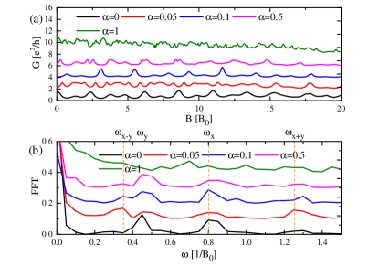
Figure 5: (a) Conductance patterns with different disorder strength $\alpha$. (b) FFT spectra of the conductance. The incident energy is $ie=0.1$ and the polar angle of the field is $\theta=\pi/6$. Other parameters are the same as those in Fig. 3.

Disorder generally exists in real samples and it can be expected that topological chiral hinge states and thus the AB effect should be robust, the same as that in the quantum Hall edge states. We show numerical results for the disorder distributed in the whole HOTI region in Fig. 5 with different strength $\alpha$. For weak disorder strength $\alpha<0.7|t|$ (the gap of the bulk states), the oscillation pattern and frequency rules $\omega_{x\pm y}=\omega_{x}\pm\omega_{y}$ retain. For strong disorder $\alpha>0.7|t|$, the oscillation pattern quenches stemming from disorder induced coupling between the surface/bulk states and the hinge states. Therefore, as long as the disorder in the sample of HOTI is not too strong, the AB effect can be hopefully observed. Similar conclusion also holds for the surface roughness. Although the AB effect is quite robust against the disorder effect, the observation should be carried out within the phase coherence length of the system. The dephasing effect always reduces the visibility of the coherent oscillation until it vanishes Golizadeh-Mojarad and Datta (2007); Lahiri et al. (2018). One more remark is that the interference here is all of the AB type without Al’tshuler-Aronov-Spivak (AAS) type contribution Al’Tshuler et al. (1981); Sharvin and Sharvin (1981); Al’tshuler et al. (1982). The model in Eq. (1) breaks time-reversal symmetry so that the AAS effect is absent.

V Summary and Outlook

In summary, we have investigated the AB effect in the chiral hinge states of the 3D HOTI. Due to the spatial configurations of the hinge states, new types of interfering loops appear compared with the 2D AB interference. Importantly, we predict a universal relationship $\omega_{x\pm y}=\omega_{x}\pm\omega_{y}$ between the dominant oscillating frequencies, which offers a unique signature of the hinge states as well as the HOTI. Our study can be generalized straightforwardly to AB effect in the 3D HOTI with helical hinge states.

Note added. Recently, we became aware of a related work Li et al. (2021), which focuses on different aspects.

Appendix A specific forms of coefficient for analysis calculation

In Eq. (5) of the main text, the coefficients are expressed as

$$\begin{split}C&=(t_{1}^{2}+t_{3}^{2})(W_{0}^{2}+W_{1}^{2}+W_{2}^{2}+X_{0}^{2}+X_{1}^{2}+X_{2}^{2})+(t_{2}^{2}+t_{4}^{2})(Y_{0}^{2}+Y_{1}^{2}+Y_{2}^{2}+Z_{0}^{2}+Z_{1}^{2}+Z_{2}^{2}),\\ C_{X}&=2(W_{0}W_{1}+X_{0}X_{1})(t_{1}^{2}+t_{3}^{2})+2(Y_{0}Y_{1}+Z_{0}Z_{1})(t_{2}^{2}+t_{4}^{2})+2(W_{0}Y_{2}+W_{2}Y_{0}+X_{0}Z_{2}+X_{2}Z_{0})(t_{1}t_{2}+t_{3}t_{4}),\\ C_{Y}&=2(W_{0}W_{2}+X_{0}X_{2})(t_{1}^{2}+t_{3}^{2})+2(Y_{0}Y_{2}+Z_{0}Z_{2})(t_{2}^{2}+t_{4}^{2})+2(W_{0}Y_{1}+W_{1}Y_{0}+X_{0}Z_{1}+X_{1}Z_{0})(t_{1}t_{2}+t_{3}t_{4}),\\ C_{XY}&=2(W_{0}Y_{0}+W_{0}Y_{0})(t_{1}t_{2}+t_{3}t_{4}),\\ C_{XY}^{\prime}&=2(W_{1}W_{2}+X_{1}X_{2})(t_{1}^{2}+t_{3}^{2})+2(Y1Y_{2}+Z_{1}Z_{2})(t_{2}^{2}+t_{4}^{2})+2(W_{1}Y_{1}+W_{2}Y_{2}+X_{1}Z_{1}+X_{2}Z_{2})(t_{1}t_{2}+t_{3}t_{4}),\\ M_{XY}&=2M_{1}M_{4}+2M_{2}M_{3},\ \ \ \ \ M_{XY}^{\prime}=2M_{1}M_{3}+2M_{2}M_{4},\ \ \ \ \ M_{2X}=2M_{1}M_{2},\ \ \ \ \ M_{2Y}=2M_{3}M_{4},\\ M_{X}&=2M_{0}M_{1}+2M_{0}M_{2},\ \ \ \ \ M_{Y}=2M_{0}M_{3}+2M_{0}M_{4},\ \ \ \ \ M_{C}=M_{0}^{2}+M_{1}^{2}+M_{2}^{2}+M_{3}^{2}+M_{4}^{2},\end{split}$$ (8)

which contain the parameters defined by the elements of the scattering matrices as

$$\begin{split}W_{0}&=t_{1}^{u},W_{1}=t_{3}^{u}r_{2}^{\prime}r_{1}^{u}-t_{1}^{u}r_{2}^{\prime}r_{3}^{u},W_{2}=t_{3}^{u}r_{4}^{\prime}r_{2}^{u}-t_{1}^{u}r_{4}^{\prime}r_{4}^{u},\\ X_{0}&=t_{2}^{u},X_{1}=t_{4}^{u}r_{2}^{\prime}r_{1}^{u}-t_{2}^{u}r_{2}^{\prime}r_{3}^{u},X_{2}=t_{4}^{u}r_{4}^{\prime}r_{2}^{u}-t_{2}^{u}r_{4}^{\prime}r_{4}^{u},\\ Y_{0}&=t_{3}^{u},Y_{1}=t_{1}^{u}r_{3}^{\prime}r_{4}^{u}-t_{3}^{u}r_{3}^{\prime}r_{2}^{u},Y_{2}=t_{1}^{u}r_{1}^{\prime}r_{3}^{u}-t_{3}^{u}r_{1}^{\prime}r_{1}^{u},\\ Z_{0}&=t_{4}^{u},Z_{1}=t_{2}^{u}r_{3}^{\prime}r_{4}^{u}-t_{4}^{u}r_{3}^{\prime}r_{2}^{u},Z_{2}=t_{2}^{u}r_{1}^{\prime}r_{3}^{u}-t_{4}^{u}r_{1}^{\prime}r_{1}^{u},\\ M_{0}&=1+r_{1}^{\prime}r_{1}^{u}r_{4}^{\prime}r_{4}^{u}+r_{3}^{\prime}r_{2}^{u}r_{2}^{\prime}r_{3}^{u}-r_{1}^{\prime}r_{3}^{u}r_{4}^{\prime}r_{2}^{u}-r_{3}^{\prime}r_{4}^{u}r_{2}^{\prime}r_{1}^{u},\\ M_{1}&=r_{2}^{\prime}r_{3}^{u},M_{2}=r_{3}^{\prime}r_{2}^{u},M_{3}=r_{4}^{\prime}r_{4}^{u},M_{4}=r_{1}^{\prime}r_{1}^{u}.\end{split}$$ (9)

References

- Qi and Zhang (2011) X.-L. Qi and S.-C. Zhang, Rev. Mod. Phys. 83, 1057 (2011).
- Hasan and Kane (2010) M. Z. Hasan and C. L. Kane, Rev. Mod. Phys. 82, 3045 (2010).
- Benalcazar et al. (2017a) W. A. Benalcazar, B. A. Bernevig, and T. L. Hughes, Science 357, 61 (2017a).
- Benalcazar et al. (2017b) W. A. Benalcazar, B. A. Bernevig, and T. L. Hughes, Phys. Rev. B 96, 245115 (2017b).
- Song et al. (2017) Z. Song, Z. Fang, and C. Fang, Phys. Rev. Lett. 119, 246402 (2017).
- Langbehn et al. (2017) J. Langbehn, Y. Peng, L. Trifunovic, F. von Oppen, and P. W. Brouwer, Phys. Rev. Lett. 119, 246401 (2017).
- Schindler et al. (2018a) F. Schindler, A. M. Cook, M. G. Vergniory, Z. Wang, S. S. Parkin, B. A. Bernevig, and T. Neupert, Science advances 4, eaat0346 (2018a).
- Franca et al. (2018) S. Franca, J. van den Brink, and I. C. Fulga, Phys. Rev. B 98, 201114 (2018).
- Park et al. (2019) M. J. Park, Y. Kim, G. Y. Cho, and S. Lee, Phys. Rev. Lett. 123, 216803 (2019).
- Khalaf (2018) E. Khalaf, Phys. Rev. B 97, 205136 (2018).
- Vu et al. (2020) D. Vu, R.-X. Zhang, and S. Das Sarma, Phys. Rev. Research 2, 043223 (2020).
- Zhang et al. (2020) R.-X. Zhang, Y.-T. Hsu, and S. Das Sarma, Phys. Rev. B 102, 094503 (2020).
- Yan (2019a) Z. Yan, Phys. Rev. Lett. 123, 177001 (2019a).
- Călugăru et al. (2019) D. Călugăru, V. Juričić, and B. Roy, Phys. Rev. B 99, 041301 (2019).
- Yan (2019b) Z. Yan, Phys. Rev. B 100, 205406 (2019b).
- Yan et al. (2018) Z. Yan, F. Song, and Z. Wang, Phys. Rev. Lett. 121, 096803 (2018).
- Schindler et al. (2018b) F. Schindler, Z. Wang, M. G. Vergniory, A. M. Cook, A. Murani, S. Sengupta, A. Y. Kasumov, R. Deblock, S. Jeon, I. Drozdov, et al., Nature physics 14, 918 (2018b).
- Liang et al. (2001) W. Liang, M. Bockrath, D. Bozovic, J. H. Hafner, M. Tinkham, and H. Park, Nature 411, 665 (2001).
- van Wees et al. (1989) B. J. van Wees, L. P. Kouwenhoven, C. J. P. M. Harmans, J. G. Williamson, C. E. Timmering, M. E. I. Broekaart, C. T. Foxon, and J. J. Harris, Phys. Rev. Lett. 62, 2523 (1989).
- Ji et al. (2003) Y. Ji, Y. Chung, D. Sprinzak, M. Heiblum, D. Mahalu, and H. Shtrikman, Nature 422, 415 (2003).
- Ofek et al. (2010) N. Ofek, A. Bid, M. Heiblum, A. Stern, V. Umansky, and D. Mahalu, Proceedings of the National Academy of Sciences 107, 5276 (2010).
- McClure et al. (2009) D. T. McClure, Y. Zhang, B. Rosenow, E. M. Levenson-Falk, C. M. Marcus, L. N. Pfeiffer, and K. W. West, Phys. Rev. Lett. 103, 206806 (2009).
- Nakamura et al. (2019) J. Nakamura, S. Fallahi, H. Sahasrabudhe, R. Rahman, S. Liang, G. C. Gardner, and M. J. Manfra, Nature Physics 15, 563 (2019).
- Henny et al. (1999) M. Henny, S. Oberholzer, C. Strunk, T. Heinzel, K. Ensslin, M. Holland, and C. Schönenberger, Science 284, 296 (1999).
- Neder et al. (2007) I. Neder, N. Ofek, Y. Chung, M. Heiblum, D. Mahalu, and V. Umansky, Nature 448, 333 (2007).
- Weisz et al. (2014) E. Weisz, H. Choi, I. Sivan, M. Heiblum, Y. Gefen, D. Mahalu, and V. Umansky, Science 344, 1363 (2014).
- Aharonov and Bohm (1959) Y. Aharonov and D. Bohm, Phys. Rev. 115, 485 (1959).
- Webb et al. (1985) R. A. Webb, S. Washburn, C. P. Umbach, and R. B. Laibowitz, Phys. Rev. Lett. 54, 2696 (1985).
- Holloway et al. (2015) G. W. Holloway, D. Shiri, C. M. Haapamaki, K. Willick, G. Watson, R. R. LaPierre, and J. Baugh, Phys. Rev. B 91, 045422 (2015).
- Lahiri et al. (2018) A. Lahiri, K. Gharavi, J. Baugh, and B. Muralidharan, Phys. Rev. B 98, 125417 (2018).
- Aleiner et al. (2015) I. L. Aleiner, A. V. Andreev, and V. Vinokur, Phys. Rev. Lett. 114, 076802 (2015).
- Tserkovnyak and Halperin (2006) Y. Tserkovnyak and B. I. Halperin, Phys. Rev. B 74, 245327 (2006).
- Peng et al. (2010) H. Peng, K. Lai, D. Kong, S. Meister, Y. Chen, X.-L. Qi, S.-C. Zhang, Z.-X. Shen, and Y. Cui, Nature materials 9, 225 (2010).
- Bardarson et al. (2010) J. H. Bardarson, P. W. Brouwer, and J. E. Moore, Phys. Rev. Lett. 105, 156803 (2010).
- Zhang and Vishwanath (2010) Y. Zhang and A. Vishwanath, Phys. Rev. Lett. 105, 206601 (2010).
- Xypakis et al. (2020) E. Xypakis, J.-W. Rhim, J. H. Bardarson, and R. Ilan, Phys. Rev. B 101, 045401 (2020).
- Li et al. (2012) J. Li, G. Fleury, and M. Büttiker, Phys. Rev. B 85, 125440 (2012).
- Ueda and Yokoyama (2014) A. Ueda and T. Yokoyama, Phys. Rev. B 90, 081405 (2014).
- Tripathi et al. (2016) K. M. Tripathi, S. Das, and S. Rao, Phys. Rev. Lett. 116, 166401 (2016).
- Bartolo et al. (2020) T. C. Bartolo, J. S. Smith, B. Muralidharan, C. Müller, T. M. Stace, and J. H. Cole, Phys. Rev. Research 2, 043430 (2020).
- Wang et al. (2016) L.-X. Wang, C.-Z. Li, D.-P. Yu, and Z.-M. Liao, Nat. Commun. 7, 10769 (2016).
- Lin et al. (2017) B.-C. Lin, S. Wang, L.-X. Wang, C.-Z. Li, J.-G. Li, D. Yu, and Z.-M. Liao, Phys. Rev. B 95, 235436 (2017).
- Kim (2006) E.-A. Kim, Phys. Rev. Lett. 97, 216404 (2006).
- Halperin et al. (2011) B. I. Halperin, A. Stern, I. Neder, and B. Rosenow, Phys. Rev. B 83, 155440 (2011).
- Willett et al. (2013) R. L. Willett, C. Nayak, K. Shtengel, L. N. Pfeiffer, and K. W. West, Phys. Rev. Lett. 111, 186401 (2013).
- Nakamura et al. (2020) J. Nakamura, S. Liang, G. C. Gardner, and M. J. Manfra, Nature Physics 16, 931 (2020).
- Jackiw and Rebbi (1976) R. Jackiw and C. Rebbi, Phys. Rev. D 13, 3398 (1976).
- Levitan and Pereg-Barnea (2020) B. A. Levitan and T. Pereg-Barnea, Phys. Rev. Research 2, 033327 (2020).
- Groth et al. (2014) C. W. Groth, M. Wimmer, A. R. Akhmerov, and X. Waintal, New Journal of Physics 16, 063065 (2014).
- Golizadeh-Mojarad and Datta (2007) R. Golizadeh-Mojarad and S. Datta, Phys. Rev. B 75, 081301 (2007).
- Al’Tshuler et al. (1981) B. Al’Tshuler, A. Aronov, and B. Spivak, JETP Lett. 33, 94 (1981).
- Sharvin and Sharvin (1981) D. Y. Sharvin and Y. V. Sharvin, JETP Lett. 34, 272 (1981).
- Al’tshuler et al. (1982) B. Al’tshuler, A. Aronov, B. Spivak, D. Y. Sharvin, and Y. V. Sharvin, JETP Lett. 35, 588 (1982).
- Li et al. (2021) C.-A. Li, S.-B. Zhang, J. Li, and B. Trauzettel, Phys. Rev. Lett. 127, 026803 (2021).