VAE²: Preventing Posterior Collapse of Variational Video Predictions in the Wild

Abstract

Predicting future frames of video sequences is challenging due to the complex and stochastic nature of the problem. Video prediction methods based on variational auto-encoders (VAEs) have been a great success, but they require the training data to contain multiple possible futures for an observed video sequence. This is hard to be fulfilled when videos are captured in the wild where any given observation only has a determinate future. As a result, training a vanilla VAE model with these videos inevitably causes posterior collapse. To alleviate this problem, we propose a novel VAE structure, dabbed VAE-in-VAE or VAE². The key idea is to explicitly introduce stochasticity into the VAE. We treat part of the observed video sequence as a random transition state that bridges its past and future, and maximize the likelihood of a Markov Chain over the video sequence under all possible transition states. A tractable lower bound is proposed for this intractable objective function and an end-to-end optimization algorithm is designed accordingly. VAE² can mitigate the posterior collapse problem to a large extent, as it breaks the direct dependence between future and observation and does not directly regress the determinate future provided by the training data. We carry out experiments on a large-scale dataset called Cityscapes, which contains videos collected from a number of urban cities. Results show that VAE² is capable of predicting diverse futures and is more resistant to posterior collapse than the other state-of-the-art VAE-based approaches. We believe that VAE² is also applicable to other stochastic sequence prediction problems where training data are lack of stochasticity.

Introduction

Video prediction finds many applications in robotics and autonomous driving, such as action recognition(Zhou et al. 2018), planning(Thrun et al. 2006), and object tracking(Guo et al. 2017). Initially, video prediction was formulated as a reconstruction problem (Ranzato et al. 2014) where the trained model regresses a determinate future for any given observation. However, real-world events are full of stochasticity. For example, a person standing may sit down, jump up, or even fall down at the next moment. A deterministic model is not capable of predicting multiple possible futures, but such capability is tremendously desired by intelligent agents as it makes them aware of different possible consequences of their actions in real applications. In order to bring stochasticity into video prediction, methods based on autoregressive models (Oord, Kalchbrenner, and Kavukcuoglu 2016), generative adversarial networks (GANs) (Goodfellow et al. 2014; Mirza and Osindero 2014), and variational auto-encoders (VAEs)(Kingma and Welling 2013) have been proposed. Among these, VAE-based methods have received the most attention and they are referred as variational video prediction (Babaeizadeh et al. 2017).

Variational video prediction learns a latent variable model that maximizes the likelihood of the data. A key to the success of variational video prediction is that the training dataset should provide multiple futures for observed frames. Not surprisingly, VAE-based video prediction methods have been using synthetic videos or scripted videos for training. These videos can provide multiple futures as desired, but they only cover a small subset of real-world scenarios. In order to build a practically applicable video prediction model, it is necessary to train it with non-scripted real-world videos such as videos captured in the wild. However, such kind of videos are usually determinate, which means only one of many possible futures is available. This situation will easily collapse a VAE model. As Fig. 1(a) shows, if there is always a unique future $v$ corresponding to each observation $I$, the hidden code $z$ becomes trivial due to the inference preference property(Chen et al. 2016). In such a case, VAE loses the capability to predict diverse futures.

VAEs are known to suffer from posterior collapse due to various reasons such as the ‘optimization challenges’(Bowman et al. 2015; Razavi et al. 2019). Although many approaches (Higgins et al. 2017; Alemi et al. 2017; Goyal et al. 2017; Razavi et al. 2019; Bowman et al. 2015) have been proposed to mitigate the problem, they hold the basic assumption that the training data have a stochastic nature. To our best knowledge, none of the previous work has looked into the model collapse problem caused by the determinate training data in video prediction. The intuition behind our solution is to explicitly inject stochasticity into the VAEs. As illustrated in Fig. 1(b), we intentionally set aside a part of the observed video sequence $I^{s}$ and treat it as a random transition state that bridges its past and future. By doing so, we can maximize the likelihood of a Markov Chain over the sequence under all possible transition states. Such formulation converts the likelihood that only relies on the observed data pairs ($I,v$) into an expectation which contains extra dependence on the distribution of the entire dataset.

However, this new formulation contains an expectation term and a likelihood term which are both intractable. To tackle it, we first derive a practical lower bound which can be optimized with a vanilla VAE structure, and then use another VAE to approximate the remaining intractable part in this lower bound. In addition, we find that the two objective functions for the two VAEs can be merged into a single expression in practice. This greatly saves the efforts to do iterative optimization. As a result, we can innovatively derive a nested VAE structure. We name this structure VAE-in-VAE, or VAE² in short. VAE² can be optimized in an end-to-end manner.

In a nutshell, the contributions of this work are: 1) We propose a novel VAE² framework to explicitly inject stochasticity into the VAE to mitigate the posterior collapse problem caused by determinate training data. 2) We turn the objective function tractable and develop an efficient end-to-end optimization algorithm. 3) We make evaluations on non-scripted real-world video prediction as well as a simple number sequence prediction task. Both quantitative and qualitative results demonstrate the efficacy of our method.

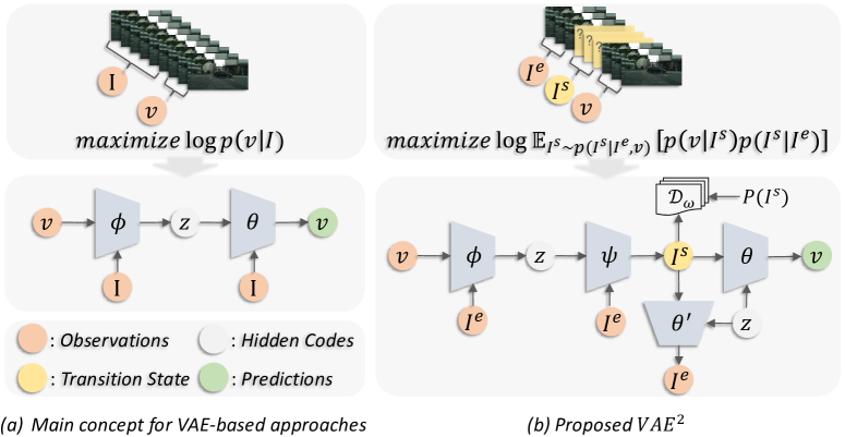
Figure 1: Schematic diagrams of vanilla VAE-based video prediction approach and our VAE² approach. $\phi$ is the encoder that maps the observation $I$ and future $v$ to a hidden random variable $z$. $\theta$ is the decoder which predicts stochastic future based on the observation and random signal sampled from $z$. When the future is determinate, the decoder $\theta$ can well reconstruct the future without accessing the random hidden code $z$. As a consequence, it leads VAE to a deterministic model. Unlike vanilla VAE that maximizes the log likelihood of determinate pair ($v$, $I$), we propose to treat part of the observation as an unknown transition state (frames $I^{s}$), and maximize the likelihood of the Markov Chain under all possible transition state. Such formulation breaks the direct dependence between future and observation, so that our method models a stochastic process. A nested VAE structure is then derived for end-to-end optimization, where $\psi$ and $\theta^{{}^{\prime}}$ are two additional decoder to produce the transition frames and reconstruct the observed frames, respectively. $D_{\omega}$ is a discriminator to help generate more realistic transitiona state frames.

Related Work

The video prediction problem can be addressed by either deterministic or non-deterministic models. Deterministic models directly reconstruct future frames with recurrent neural networks(Ranzato et al. 2014; Oh et al. 2015; Srivastava, Mansimov, and Salakhudinov 2015; Villegas et al. 2017; Finn, Goodfellow, and Levine 2016; Lu, Hirsch, and Scholkopf 2017) or feed-forward networks(Jia et al. 2016; Vondrick and Torralba 2017; Liu et al. 2017; Walker, Gupta, and Hebert 2015). The reconstruction loss assumes a deterministic environment. Such models cannot capture the stochastic nature in real world videos and usually result in an averaged prediction over all possibilities.

Non-deterministic models can be further classified into autoregressive models, GANs, and VAEs. In pixel-level autoregressive models(Oord, Kalchbrenner, and Kavukcuoglu 2016), spatiotemporal dependencies are jointly modeled, where each pixel in the predicted video frames fully depends on the previously predicted pixel via chain rule (Kalchbrenner et al. 2017). Although autoregressive model can directly construct video likelihood through full factorization over each pixel, it is unpractical due to its high inference complexity. Besides, it has been observed to fail on globally coherent structures(Razavi et al. 2019) and generate very noisy predictions (Babaeizadeh et al. 2017). GANs(Goodfellow et al. 2014) and conditional GANs (c-GANs)(Mirza and Osindero 2014) are also employed for stochastic video prediction, for their capability to generate data close to the target distribution. GAN-based approaches can predict sharp and realistic video sequences(Vondrick, Pirsiavash, and Torralba 2016), but is prone to model collapse and often fails to produce diverse futures(Lee et al. 2018).

VAE-based models have received the most attention among the non-deterministic models. In particular, conditional VAEs (c-VAEs) have been shown to be able to forecast diverse future actions a single static image (Walker et al. 2016; Xue et al. 2016). c-VAEs have also been used to predict diverse future sequences from an observed video sequence (Babaeizadeh et al. 2017; Lee et al. 2018; Denton and Fergus 2018; Minderer et al. 2019). In some of these approaches, human body skeleton(Minderer et al. 2019) and dense trajectory(Walker et al. 2016) are incorporated in addition to the RGB frames to enhance the prediction quality. Besides, RNN-based encoder-decoder structures such as LSTM(Hochreiter and Schmidhuber 1997) has also been employed for long-term predictions(Wichers et al. 2018). Some other works leverage GANs to further boost the visual quality(Lee et al. 2018).

So far, the success of VAE-based video prediction methods has been limited to synthetic videos or scripted videos, such as video games or synthetic shapes rendered with multiple futures(Xue et al. 2016; Babaeizadeh et al. 2017), BAIR robotic pushing dataset(Ebert et al. 2017) with randomly moving robotic arms that conduct multiple possible movements(Babaeizadeh et al. 2017; Lee et al. 2018), or KTH(Schuldt, Laptev, and Caputo 2004) and Human3.6M(Ionescu et al. 2013) where one volunteer repeatedly conducts predefined activities (such as hand clapping and walking) in well controlled environments(Lee et al. 2018; Denton and Fergus 2018; Babaeizadeh et al. 2017; Minderer et al. 2019). In these datasets, multiple futures are created for a given observation, so that the VAE model can be trained as desired. However, videos captured in the wild are usually determinate. There is always a unique future for a given observation. Such a data distribution can easily result in posterior collapse and degenerate VAE to a deterministic model. A possible fix is to treat future frames at multiple time steps as multiple futures at a single time step(Xue et al. 2016; Walker et al. 2016), but such manipulation creates a non-negligible gap between the distributions of the training data and the real-world data. In this paper, we propose VAE² to alleviate the posterior collapse problem in variational video prediction. Different from previous attempts that address model collapse in VAEs such as employing weak decoder(Bowman et al. 2015; Gulrajani et al. 2016), involving stronger constraints(Higgins et al. 2017; Goyal et al. 2017) or annealing strategy(Kim et al. 2018; Gulrajani et al. 2016; Bowman et al. 2015), VAE² is specially designed to handle the collapse problem caused by videos lacking of stochasticity.

VAE-in-VAE

In this section, we elaborate the proposed VAE² step by step. We start with introducing the VAE’s posterior collapse in video prediction caused by the determinate data pair. Next, we describe how to overcome this problem by injecting stochasticity into vanilla VAE’s objective function. Then, we propose a tractable lower bound to facilitate gradient-based solution and finally derive the VAE-in-VAE structure for end-to-end optimization.

Posterior Collapse of Vanilla VAE with Determinate Data Pair

We first briefly introduce the formulation of traditional VAE-based solutions for video predictions. Let $\mathcal{D}=\{(I_{k},v_{k})\}$ denote some i.i.d. data pairs consisting of $K$ samples. Assuming $v$ is conditioned on $I$ with some random processes involving an unobserved hidden variable $z$, one can maximize the conditional data likelihood $\sum_{k=1}^{K}\log p(v_{k}\mid I_{k})$ with conditioned VAEs (c-VAEs) through maximizing the variational lower bound

$$\mathbb{E}_{q_{\phi}(z_{k}\mid I_{k},v_{k})}[p_{\theta}(v_{k}\mid I_{k},z_{k})]-KL(q_{\phi}(z_{k}\mid I_{k},v_{k})\mid\mid p(z)),$$ (1)

where $q_{\phi}$ is a parametric model that approximates the true posterior $p(z_{k}\mid I_{k},v_{k})$, $p_{\theta}$ is a generative model w.r.t. the hidden code $z_{k}$ and the data $I_{k}$. $KL$ denotes the Kullback-Leibler(KL) Divergence.

When VAE is used for stochastic video prediction, each $I_{k}\in\mathbb{R}^{T_{I}\times H\times W}$ represents an observed video sequence consisting of $T_{I}$ consecutive frames with $H\times W$ spatial size, $v_{k}\in\mathbb{R}^{T_{v}\times H\times W}$ is the future sequence of the observation consisting of $T_{v}$ consecutive frames. A general framework for variational video prediction is illustrated in Fig. 1 (a), where an encoder $\phi$ and a decoder $\theta$ are employed to instantiate $q_{\phi}$ and $p_{\theta}$, respectively.

In Eq. 1, there is a regression term $p_{\theta}(v_{k}\mid I_{k},z_{k})$ which is usually modeled by a deep decoder that takes as inputs the observation $I_{k}$ and hidden code $z_{k}$ and directly regresses the future $v_{k}$. Since the videos in the wild are determinately captured, each $I_{k}$ is only associated with a unique $v_{k}$ without stochasticity. In principle, such determinate data pair $(I_{k},v_{k})$ can be easily fit by the decoder $\theta$ since networks with sufficient capacity are capable of representing arbitrarily complex functions(Hornik et al. 1989) or even memorize samples(Arpit et al. 2017). Therefore, the hidden code $z$ can be entirely ignored by the decoder to fulfill the KL divergence term based on the information preference property(Chen et al. 2016). As a result, VAE is modeling a deterministic process under this scenario.

From VAE to VAE² by Introducing Stochasticity

The reason for the aforementioned collapse issue is that traditional c-VAEs maximize the likelihood $p(v_{k}\mid I_{k})$ over data pair $(v_{k},i_{k})$ which has no stochastic behavior. The key to avoid such collapse is to ensure that the VAE is modeling a stochastic process instead of a deterministic one. To achieve this, we split each observation $I_{k}$ into two parts: determinate observation $I^{e}_{k}\in\mathbb{R}^{\frac{T_{I}}{2}\times H\times W}$ and random transition state $I^{s}_{k}\in\mathbb{R}^{\frac{T_{I}}{2}\times H\times W}$. Different from the determinate $I^{e}_{k}$, $I^{s}_{k}$ is treated as a random event that bridges the determinate observation and the unknown future. Assuming that evolution of a video sequence subjects to a Markov process, where the generation process of a sequence is only conditioned on its previous sequence, we propose to maximize the likelihood of the Markov Chain over observations and futures under all possible transition states. The optimization problem can be expressed as

$$maximize~{}\log\mathbb{E}_{p(I^{s}_{k}\mid v_{k},I^{e}_{k})}[p(v_{k}\mid I^{s}_{k})p(I^{s}_{k}\mid I^{e}_{k})].$$ (2)

Intuitively, the proposed objective function involves stochastic information by explicitly relaxing a part of determinate observations to random transition state. However, such formulation is intractable in terms of both the likelihood of the Markov Chain and the expectation term.

A Tractable Objective Function for VAE²

In this section, we demonstrate that a tractable lower bound for Eq. 2 can be derived by applying Cauchy-Schwarz inequality. Specifically, we have

$$\begin{split}&\log\mathbb{E}_{p(I^{s}\mid v,I^{e})}[p(v\mid I^{s})p(I^{s}\mid I^{e})]\\ &\geq\mathbb{E}_{q_{\phi}(z\mid I^{e},v)}[\log\mathbb{E}_{p(I^{s}\mid I^{e},z)}p_{\theta}(v\mid I^{s},z)]\\ &~{}~{}~{}~{}~{}~{}~{}~{}-KL(q_{\phi}(z\mid I^{e},v)\mid\mid p(z)).\\ \end{split}$$ (3)

Here we omit index $k$ for simplicity. The above lower bound serves as our first-level objective function. It has a similar form as Eq. 1 except that we have one additional transition variable $I^{s}$ in the decoder model $p_{\theta}$. To maximize this lower bound, we need to calculate the expectation term $\mathbb{E}_{p(I^{s}\mid I^{e},z)}p_{\theta}(v\mid I^{s},z)$ in Eq. 3, which requires an approximation towards $p(I^{s}\mid I^{e},z)$. Here, we employ a generation model $q_{\psi}(I^{s}\mid I^{e},z)$ parameterized with $\psi$ for the approximation by minimizing $KL(q_{\psi}(I^{s}\mid I^{e},z)\mid\mid p(I^{s}\mid I^{e},z))$, which induces our second-level objective function

$$\mathbb{E}_{q_{\psi}(I^{s}\mid I^{e},z)}\log p_{\theta^{{}^{\prime}}}(I^{e}\mid I^{s},z)-KL(q_{\psi}(I^{s}\mid I^{e},z)\mid\mid p(I^{s})).$$ (4)

For the full derivation of Eq. 3 and Eq. 4, please refer to our appendix. Since transition state $I^{s}$ is high-dimensional signals (video sequences), the exact functional form of its prior distribution is not accessible. We follow adversarial autoencoders(Makhzani et al. 2015) to leverage adversarial training to minimize the distance between the $q_{\psi}(I^{s}\mid I^{e},z)$ and the prior $p(I^{s})$. As such, $-KL(q_{\psi}(I^{s}\mid I^{e},z)\mid\mid p(I^{s}))$ in Eq. 4 is replaced by

$$D_{\omega}(I^{s},I_{prior}),~{}where~{}I_{prior}\sim p(I^{s}),I^{s}\sim q_{\psi}(I^{s}\mid I^{e},z).$$ (5)

Here, $D_{\omega}$ is a discriminator network parameterized with $\omega$ and $I_{prior}$ is randomly sampled from the video dataset. By doing so, the second-level objective function Eq. 4 is now tractable. Ideally, we shall optimize the first-level and second-level objective function iteratively, which requires unaffordable training time for convergence. In practice, we simplify such iterative learning process by merging the two objective functions into a single one as

$$\begin{split}&\mathcal{L}(I^{e},I^{s},v;\theta,\phi)+\\ &\lambda[\mathbb{E}_{q_{\psi}(I^{s}\mid I^{e},z)}\log p_{\theta^{{}^{\prime}}}(I^{e}\mid I^{s},z)+{D}_{\omega}(I^{s},I_{prior})],\end{split}$$ (6)

where $\lambda$ is a loss weight applied on Eq. 4. This simplification enables us to simultaneously optimize the two objective functions and we use a weight $\lambda$ to adjust the optimization speed of our second-level objective function to mimic the original iterative process.

End-to-end Optimization

We employ two VAE structures to maximize our final objective function in Eq. 6. As illustrated in Fig. 1(b), the first VAE consisting of an encoder $\phi$ and a decoder $\theta$ is incorporated to maximize the first-level objective function $\mathcal{L}(I^{e},I^{s},v;\theta,\phi)$. The second VAE with an encoder $\psi$, a decoder ${\theta^{{}^{\prime}}}$ and a discriminator $D_{\omega}$ is used for maximizing the second-level objective function. We assume $p_{\theta}$ and $p_{\theta^{{}^{\prime}}}$ to be Laplace distribution (which leads to L1 regression loss) and assume $q_{\phi}$ to be Gaussian. The training procedure can be summarized as follows:

• Encoder $\phi$ takes $I^{e}$ and $v$ as inputs and produces hidden codes $z$. $z$ is fed into $\psi$ to generate $L$ different $I^{s}$. For each $I^{s}$, decoder $\theta$ and $\theta^{{}^{\prime}}$ reconstruct $v$ and $I^{e}$, respectively.

• Estimate the $\log\mathbf{E}_{p(I^{s}\mid I^{e},z)}p_{\theta}(v\mid I^{s},z)$ in Eq. 3 with $\log\sum_{i=1}^{L}p_{\theta}(v\mid I^{s}_{i},z)$. Estimate $\mathbf{E}_{q_{\psi}(I^{s}\mid I^{e},z)}\log p_{\theta^{{}^{\prime}}}(I^{e}\mid I^{s},z)$ in Eq. 6 with $\sum_{i=1}^{L}\log p_{\theta^{{}^{\prime}}}(I^{e}\mid I^{s}_{i},z)$.

• Compute gradients w.r.t. Eq. 6 and update $\phi$, $\psi$, $\theta$, $\theta^{{}^{\prime}}$. Update $D_{\omega}$ with adversarial learning.

In practice, we observe that this simplified process works well even with $L=1$. This further reduces the algorithm complexity.

Number Sequence Prediction

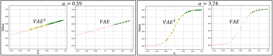
Figure 2: Visualization of the number sequence prediction at two model parameters. The 100 predictions made by VAE baseline are almost identical while those made by the proposed VAE² are more scattered around the groundtruth. This shows that VAE² captures the inherent stochastic law of the number sequences model.

We first use a simple number sequence prediction task to demonstrate how VAE² mitigates the collapse problem when only determinate data are available. More specifically, we explicitly design a world model which can stochastically produce number sequences w.r.t. the given model parameter.

Sequence Model Design. The stochastic model that generates number sequence is defined by $G(\alpha,H(\boldsymbol{\epsilon}))=\frac{1}{1+e^{-\alpha H(\boldsymbol{\epsilon})}}$. Here, $H(\boldsymbol{\epsilon})=[h_{0}(\epsilon_{0}),h_{1}(\epsilon_{1}),...,h_{N-1}(\epsilon_{N-1})]\in\mathbb{R}^{N}$ and $h_{i}(\epsilon_{i})=C+i*S+\epsilon_{i}$, where $\epsilon_{i}\sim Uniform(0,S)$. This world model is parameterized by $\alpha$ and its stochastic nature is characterized by $H(\boldsymbol{\epsilon})$.

Constructing the Dataset. In order to mimic the determinate video sequences captured in the wild, we use $G(\alpha,H(\epsilon))$ to generate only one number sequence for each world parameter $\alpha$. We then split each number sequence into three even parts. For VAE², the three parts correspond to $I^{e}$, $I^{s}$ and $v$, respectively. For the baseline VAE, the first and the second parts together correspond to $I$ and the third part corresponds to $v$. The dataset $D=\{G(\alpha_{k},H(\boldsymbol{\hat{\epsilon}})),k\in[1,K]\}$ contains $K$ number sequences generated from $K$ different world model parameters, where $H(\boldsymbol{\hat{\epsilon}})$ denotes a single sampling result of $H(\boldsymbol{\epsilon)}$. We set $C$, $S$, $N$, and $K$ to -1.5, 0.1, 30 and 10,000, respectively. The constructed dataset contains 10,000 number sequences, each of which has 30 data points.

Evaluation and Visualization. We train our VAE², VAE(Babaeizadeh et al. 2017) and VAE-GAN(Lee et al. 2018) models on this number sequence dataset, respectively. The training and architecture details can be found in the appendix. After training, we make 100 predictions on $v$ using each method. In Fig. 2, we plot original data points in red and predicted ones in green. The different shapes correspond to different hidden variables $h_{i}(\epsilon_{i})$.

We observe from the figure that the predicted $v$ from the baseline VAE model are almost identical among the 100 predictions (samples of the same shape are grouped together), showing that the baseline VAE degrades to a deterministic model. In contrast, the proposed VAE² provides much more diverse predictions (samples of each shape scatter around the ground-truth). Although we do not provide multiple futures in the training dataset, VAE² is able to explore the underlying stochastic information through our innovative design. More visualizations can be found in the appendix.

In addition to visualizing the predicted numbers, we can use the standard deviation of the L1 loss of different samples to measure the diversity of predictions. Fig. 3(a) plots the mean and the standard deviation of the predictions from VAE² and its counterparts on the entire dataset. It is clear that the number sequences predicted by the proposed VAE² are more diverse than other methods.

Experiments on Videos Captured in the Wild

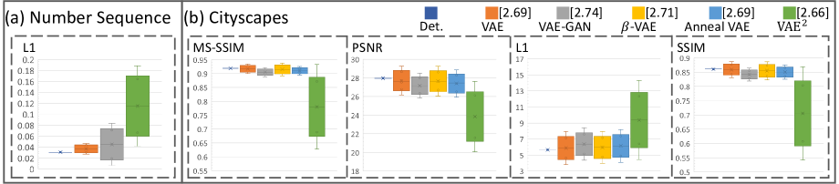
Figure 3: Standard deviation of 100 prediction samples from different methods under four criteria. Each box and whisker indicates the mean $\pm$ three times and five times standard deviation, respectively. Larger deviation range of VAE² indicates it can significantly improve the diversity of the predictions. The number beside each legend denotes the averaged Inception Score of the 100 samples from corresponding method over the entire Cityscapes dataset.

Dataset and Evaluation Metrics. We evaluate the proposed VAE² with the Cityscapes dataset(Cordts et al. 2016) which contains urban street scenes from 50 different cities. The videos are captured at 17 fps with cameras mounted on moving cars. Since a car and its mounted camera pass each street only once, every video sequence is determinate and there are no multiple futures available. The average number of humans and vehicles per frame is 7.0 and 11.8, respectively, providing a fairly complex instance pattern.

There is no consensus yet on how to evaluate a video prediction scheme. Previous work has tried to evaluate the perceived visual quality of the predicted frames. However, this work is focused on mitigating the model collapse problem caused by determinate training data. In addition to the perceived visual quality, we will mainly evaluate how seriously a prediction model suffers from the model collapse problem. In general, the more diverse the predicted frames are, the better the model handles the model collapse problem. The diversity of predicted frames can be evaluated both quantitatively and qualitatively. In particular, we use the standard deviation of some conventional image quality evaluation metrics, such as SSIM(Wang et al. 2004), PSNR(Huynh-Thu and Ghanbari 2008), and L1 loss, for quantitative evaluation. We also compute the optical flows between the ground-truth future frame and the predicted future frames by various prediction models. Since optical flow reflects per-pixel displacement, it can be a very intuitive way to show the pixel-level difference between the two frames.

Reference Schemes and Implementation Details. Existing VAE-based video prediction approaches are designed with different backbone networks and data structures, including RGB frames, skeleton, or dense trajectory. In this work, we only consider methods that directly operate on raw RGB videos to demonstrate the efficacy of the proposed VAE². These prediction models can be categorized into two VAE variants, namely vanilla VAEs (Babaeizadeh et al. 2017; Xue et al. 2016; Denton and Fergus 2018) and VAE-GAN (Lee et al. 2018; Larsen et al. 2015). In addition, we evaluate $\beta$-VAE(Higgins et al. 2017) and VAE with annealing(Bowman et al. 2015) which are designed for addressing the model collapse problem without considering the situation where training data lack of stochasticity. We also construct a deterministic model as a baseline.

We employ 18-layer HRNet (wd-18-small)(Sun et al. 2019) to instantiate all the encoders, decoders, and GANs in VAE². For fair comparison, we replace the original backbone network in the reference schemes (Babaeizadeh et al. 2017; Lee et al. 2018; Higgins et al. 2017; Bowman et al. 2015) with the same HRNet. The deterministic baseline is also a 18-layer HRNet which directly regresses the future frames. We set $\lambda$ to 0.1 and we use Adam optimizer to train all methods for 1,000 epochs. More training details can be found in the appendix.

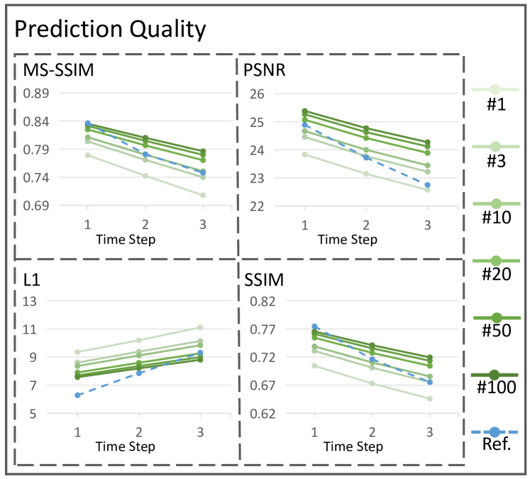
Figure 4: Prediction qualities under different numbers of samples. VAE² can generate predictions very close to the ground truth future when it is sampled for sufficient times.

Diversity and Quality. In order to measure the diversity of the predictions, we make 100 random predictions with each method and compute the PSNR, L1 distance, SSIM, and multi-scale SSIM (MS-SSIM)(Wang, Simoncelli, and Bovik 2003) between each predicted frame and the ground-truth future frame. In Fig. 3, we use box-and-whisker charts to plot the mean (the center of each box), the 3-sigma (solid box), and the 5-sigma (whiskers) of each metric, where sigma denotes the standard deviation. In each sub-figure, different colors represent different methods. It is clear from the figure that the future frames predicted by VAE² have a larger standard deviation than the reference schemes. It corroborates that VAE² can predict much more diverse futures than existing methods. Besides, we can find that approaches such as $\beta$-VAE and Anneal-VAE that are designed for model collapse fail in this scenario. They only bring marginal diversity improvement. This implies that we need a specific solution like VAE² when source data lack stochasticity.

Another intuitive way to check whether the proposed VAE² helps alleviate the model collapse problem is to evaluate the KL loss of the hidden code $z$. A variational model that collapses to its deterministic counterpart usually has a very small KL loss. As can be viewed in Fig. 5, the converged KL loss of counterpart methods is significantly smaller than that of VAE².

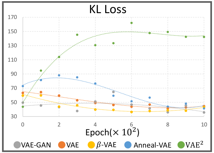
Figure 5: KL loss (without normalization) of the latent variable $z$ during training for different schemes. Small KL loss indicates the learned distribution of the hidden variable $z$ is very close to the prior distribution. When KL loss approaches to zero, the latent variable does not encode any useful information.

Finally, we follow the methods in (Babaeizadeh et al. 2017) to evaluate the video prediction quality. In Fig. 4, we plot the best prediction among different numbers of samples under various metrics. The reference is a deterministic model(Finn, Goodfellow, and Levine 2016) that directly regresses the ground-truth future. We can see from the figure that as the number of samples increases, the proposed VAE² can predict video sequences at a quality that is comparable with the reference model in terms of the reconstruction fidelity. As the time-step increases, VAE² achieves an even better performance than the reference. We also employ Inception Score(IS)(Salimans et al. 2016), a frequently used no-reference image quality assessment method, to measure the visual quality of the predicted futures. As illustrated by the number beside each legend in Fig. 3, the scores are close to each other, which suggests the overall visual quality of the futures predicted by VAE² are on par with other approaches.

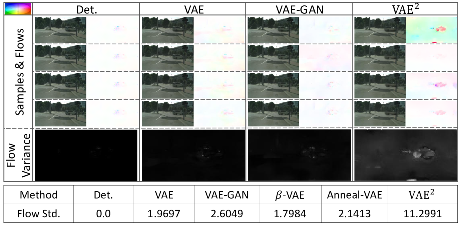
Figure 6: Visualization of predictions and their corresponding optical flow w.r.t. the ground-truth future. We randomly sample four futures with each method. The diverse patterns of the flow images under VAE² indicate its stochastic behavior. The last row shows the standard deviations of the flow images over 100 samples. The large value of VAE² supports that it predicts much more diverse future. More visualizations can be found in the appendix.

Visualizations. Due to limited space, we only visualize single frame predictions with three baseline methods in this section. More visualizations can be found in the appendix. Fig. 7 shows three sampled predictions of a single prediction step for each of the schemes to be compared. We notice that the future positions of the fast moving truck predicted by VAE(Babaeizadeh et al. 2017) and VAE-GAN(Lee et al. 2018) are almost identical to the deterministic baseline. There is little stochasticity among different samples. In contrast, VAE² achieves noticeable randomness on the moving truck and the moving camera. The predicted camera motion can be observed from the parking car on the right.

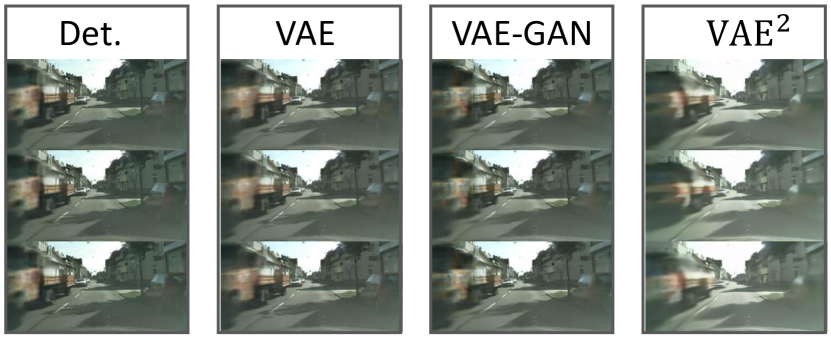
Figure 7: Visualization of three predictions for the next frame of an observed video sequence. Each column contains the three predictions made by each method. It can be observed that VAE² predicts quite different futures while the others make almost identical predictions.

In order to show the detailed difference among predictions, we compute and colorize(Baker et al. 2011) the optical flow between each prediction and the ground-truth future frame. In Fig. 6, we show four predictions of each method and their corresponding optical flow. The color code for optical flows is illustrated at the top-left corner. For example, the first flow map under VAE² has a green hue, suggesting that the whole background shifts left w.r.t. the ground truth future. This means the camera car is predicted to turn right in the coming future (although it is not the ground-truth future in the dataset). It can also be observed that the displacement patterns of the frames predicted by our method are much more diverse than the other approaches. To quantify such diversity, we compute and visualize the (normalized) standard deviation of the optical flows on 100 different samples for each method. As can be viewed in fifth row, the flow variance of VAE² has much larger responses on the moving car and the whole background region. The statistics of such diversity on the entire dataset are presented in the table at the last row to illustrate the efficacy of VAE² on predicting stochastic futures.

Conclusion and Discussion

In this paper, we investigate the posterior collapse problem in variational video prediction caused by the videos determinately captured in the wild. We effectively mitigate this problem by explicitly introducing stochasticity into vanilla VAEs and propose an end-to-end framework, VAE², for optimization. The proposed VAE² demonstrates its capability of capturing the stochastic information of videos in the wild, which makes variational video prediction more practical in real-world applications. In addtition, we believe that VAE² can be effectively extended to other sequential prediction problems where training data are lack of stochasticity. We will leave this part to future works.

We also notice that the inference structure of VAE² looks similar to the recently proposed two-stage VAE (Dai and Wipf 2019). However, this two-stage VAE is designed to address the problem that the hidden code drawn from the encoder is incongruous with the prior, and the first VAE is used to predict the distribution of the hidden code instead of the randomized partial observation as in VAE².

References

- Alemi et al. (2017) Alemi, A. A.; Poole, B.; Fischer, I.; Dillon, J. V.; Saurous, R. A.; and Murphy, K. 2017. Fixing a broken ELBO. arXiv preprint arXiv:1711.00464 .
- Arpit et al. (2017) Arpit, D.; Jastrzebski, S.; Ballas, N.; Krueger, D.; Bengio, E.; Kanwal, M. S.; Maharaj, T.; Fischer, A.; Courville, A.; Bengio, Y.; et al. 2017. A closer look at memorization in deep networks. arXiv preprint arXiv:1706.05394 .
- Babaeizadeh et al. (2017) Babaeizadeh, M.; Finn, C.; Erhan, D.; Campbell, R. H.; and Levine, S. 2017. Stochastic variational video prediction. arXiv preprint arXiv:1710.11252 .
- Baker et al. (2011) Baker, S.; Scharstein, D.; Lewis, J.; Roth, S.; Black, M. J.; and Szeliski, R. 2011. A database and evaluation methodology for optical flow. International journal of computer vision 92(1): 1–31.
- Bowman et al. (2015) Bowman, S. R.; Vilnis, L.; Vinyals, O.; Dai, A. M.; Jozefowicz, R.; and Bengio, S. 2015. Generating sentences from a continuous space. arXiv preprint arXiv:1511.06349 .
- Chen et al. (2016) Chen, X.; Kingma, D. P.; Salimans, T.; Duan, Y.; Dhariwal, P.; Schulman, J.; Sutskever, I.; and Abbeel, P. 2016. Variational lossy autoencoder. arXiv preprint arXiv:1611.02731 .
- Cordts et al. (2016) Cordts, M.; Omran, M.; Ramos, S.; Rehfeld, T.; Enzweiler, M.; Benenson, R.; Franke, U.; Roth, S.; and Schiele, B. 2016. The cityscapes dataset for semantic urban scene understanding. In Proceedings of the IEEE conference on computer vision and pattern recognition, 3213–3223.
- Dai and Wipf (2019) Dai, B.; and Wipf, D. 2019. Diagnosing and enhancing vae models. arXiv preprint arXiv:1903.05789 .
- Denton and Fergus (2018) Denton, E.; and Fergus, R. 2018. Stochastic video generation with a learned prior. arXiv preprint arXiv:1802.07687 .
- Ebert et al. (2017) Ebert, F.; Finn, C.; Lee, A. X.; and Levine, S. 2017. Self-supervised visual planning with temporal skip connections. arXiv preprint arXiv:1710.05268 .
- Finn, Goodfellow, and Levine (2016) Finn, C.; Goodfellow, I.; and Levine, S. 2016. Unsupervised learning for physical interaction through video prediction. In Advances in neural information processing systems, 64–72.
- Goodfellow et al. (2014) Goodfellow, I.; Pouget-Abadie, J.; Mirza, M.; Xu, B.; Warde-Farley, D.; Ozair, S.; Courville, A.; and Bengio, Y. 2014. Generative adversarial nets. In Advances in neural information processing systems, 2672–2680.
- Goyal et al. (2017) Goyal, A. G. A. P.; Sordoni, A.; Côté, M.-A.; Ke, N. R.; and Bengio, Y. 2017. Z-forcing: Training stochastic recurrent networks. In Advances in neural information processing systems, 6713–6723.
- Gulrajani et al. (2016) Gulrajani, I.; Kumar, K.; Ahmed, F.; Taiga, A. A.; Visin, F.; Vazquez, D.; and Courville, A. 2016. Pixelvae: A latent variable model for natural images. arXiv preprint arXiv:1611.05013 .
- Guo et al. (2017) Guo, Q.; Feng, W.; Zhou, C.; Huang, R.; Wan, L.; and Wang, S. 2017. Learning dynamic siamese network for visual object tracking. In Proceedings of the IEEE International Conference on Computer Vision, 1763–1771.
- Higgins et al. (2017) Higgins, I.; Matthey, L.; Pal, A.; Burgess, C.; Glorot, X.; Botvinick, M.; Mohamed, S.; and Lerchner, A. 2017. beta-VAE: Learning Basic Visual Concepts with a Constrained Variational Framework. Iclr 2(5): 6.
- Hochreiter and Schmidhuber (1997) Hochreiter, S.; and Schmidhuber, J. 1997. Long short-term memory. Neural computation 9(8): 1735–1780.
- Hornik et al. (1989) Hornik, K.; Stinchcombe, M.; White, H.; et al. 1989. Multilayer feedforward networks are universal approximators. Neural networks 2(5): 359–366.
- Huynh-Thu and Ghanbari (2008) Huynh-Thu, Q.; and Ghanbari, M. 2008. Scope of validity of PSNR in image/video quality assessment. Electronics letters 44(13): 800–801.
- Ionescu et al. (2013) Ionescu, C.; Papava, D.; Olaru, V.; and Sminchisescu, C. 2013. Human3. 6m: Large scale datasets and predictive methods for 3d human sensing in natural environments. IEEE transactions on pattern analysis and machine intelligence 36(7): 1325–1339.
- Jia et al. (2016) Jia, X.; De Brabandere, B.; Tuytelaars, T.; and Gool, L. V. 2016. Dynamic filter networks. In Advances in Neural Information Processing Systems, 667–675.
- Kalchbrenner et al. (2017) Kalchbrenner, N.; van den Oord, A.; Simonyan, K.; Danihelka, I.; Vinyals, O.; Graves, A.; and Kavukcuoglu, K. 2017. Video pixel networks. In Proceedings of the 34th International Conference on Machine Learning-Volume 70, 1771–1779. JMLR. org.
- Kim et al. (2018) Kim, Y.; Wiseman, S.; Miller, A. C.; Sontag, D.; and Rush, A. M. 2018. Semi-amortized variational autoencoders. arXiv preprint arXiv:1802.02550 .
- Kingma and Welling (2013) Kingma, D. P.; and Welling, M. 2013. Auto-encoding variational bayes. arXiv preprint arXiv:1312.6114 .
- Larsen et al. (2015) Larsen, A. B. L.; Sønderby, S. K.; Larochelle, H.; and Winther, O. 2015. Autoencoding beyond pixels using a learned similarity metric. arXiv preprint arXiv:1512.09300 .
- Lee et al. (2018) Lee, A. X.; Zhang, R.; Ebert, F.; Abbeel, P.; Finn, C.; and Levine, S. 2018. Stochastic adversarial video prediction. arXiv preprint arXiv:1804.01523 .
- Liu et al. (2017) Liu, Z.; Yeh, R. A.; Tang, X.; Liu, Y.; and Agarwala, A. 2017. Video frame synthesis using deep voxel flow. In Proceedings of the IEEE International Conference on Computer Vision, 4463–4471.
- Lu, Hirsch, and Scholkopf (2017) Lu, C.; Hirsch, M.; and Scholkopf, B. 2017. Flexible spatio-temporal networks for video prediction. In Proceedings of the IEEE Conference on Computer Vision and Pattern Recognition, 6523–6531.
- Makhzani et al. (2015) Makhzani, A.; Shlens, J.; Jaitly, N.; Goodfellow, I.; and Frey, B. 2015. Adversarial autoencoders. arXiv preprint arXiv:1511.05644 .
- Minderer et al. (2019) Minderer, M.; Sun, C.; Villegas, R.; Cole, F.; Murphy, K. P.; and Lee, H. 2019. Unsupervised learning of object structure and dynamics from videos. In Advances in Neural Information Processing Systems, 92–102.
- Mirza and Osindero (2014) Mirza, M.; and Osindero, S. 2014. Conditional generative adversarial nets. arXiv preprint arXiv:1411.1784 .
- Oh et al. (2015) Oh, J.; Guo, X.; Lee, H.; Lewis, R. L.; and Singh, S. 2015. Action-conditional video prediction using deep networks in atari games. In Advances in neural information processing systems, 2863–2871.
- Oord, Kalchbrenner, and Kavukcuoglu (2016) Oord, A. v. d.; Kalchbrenner, N.; and Kavukcuoglu, K. 2016. Pixel recurrent neural networks. arXiv preprint arXiv:1601.06759 .
- Ranzato et al. (2014) Ranzato, M.; Szlam, A.; Bruna, J.; Mathieu, M.; Collobert, R.; and Chopra, S. 2014. Video (language) modeling: a baseline for generative models of natural videos. arXiv preprint arXiv:1412.6604 .
- Razavi et al. (2019) Razavi, A.; Oord, A. v. d.; Poole, B.; and Vinyals, O. 2019. Preventing posterior collapse with delta-vaes. arXiv preprint arXiv:1901.03416 .
- Salimans et al. (2016) Salimans, T.; Goodfellow, I.; Zaremba, W.; Cheung, V.; Radford, A.; and Chen, X. 2016. Improved techniques for training gans. In Advances in neural information processing systems, 2234–2242.
- Schuldt, Laptev, and Caputo (2004) Schuldt, C.; Laptev, I.; and Caputo, B. 2004. Recognizing human actions: a local SVM approach. In Proceedings of the 17th International Conference on Pattern Recognition, 2004. ICPR 2004., volume 3, 32–36. IEEE.
- Srivastava, Mansimov, and Salakhudinov (2015) Srivastava, N.; Mansimov, E.; and Salakhudinov, R. 2015. Unsupervised learning of video representations using lstms. In International conference on machine learning, 843–852.
- Sun et al. (2019) Sun, K.; Xiao, B.; Liu, D.; and Wang, J. 2019. Deep high-resolution representation learning for human pose estimation. In Proceedings of the IEEE Conference on Computer Vision and Pattern Recognition, 5693–5703.
- Thrun et al. (2006) Thrun, S.; Montemerlo, M.; Dahlkamp, H.; Stavens, D.; Aron, A.; Diebel, J.; Fong, P.; Gale, J.; Halpenny, M.; Hoffmann, G.; et al. 2006. Stanley: The robot that won the DARPA Grand Challenge. Journal of field Robotics 23(9): 661–692.
- Villegas et al. (2017) Villegas, R.; Yang, J.; Hong, S.; Lin, X.; and Lee, H. 2017. Decomposing motion and content for natural video sequence prediction. arXiv preprint arXiv:1706.08033 .
- Vondrick, Pirsiavash, and Torralba (2016) Vondrick, C.; Pirsiavash, H.; and Torralba, A. 2016. Generating videos with scene dynamics. In Advances in neural information processing systems, 613–621.
- Vondrick and Torralba (2017) Vondrick, C.; and Torralba, A. 2017. Generating the future with adversarial transformers. In Proceedings of the IEEE Conference on Computer Vision and Pattern Recognition, 1020–1028.
- Walker et al. (2016) Walker, J.; Doersch, C.; Gupta, A.; and Hebert, M. 2016. An uncertain future: Forecasting from static images using variational autoencoders. In European Conference on Computer Vision, 835–851. Springer.
- Walker, Gupta, and Hebert (2015) Walker, J.; Gupta, A.; and Hebert, M. 2015. Dense optical flow prediction from a static image. In Proceedings of the IEEE International Conference on Computer Vision, 2443–2451.
- Wang et al. (2004) Wang, Z.; Bovik, A. C.; Sheikh, H. R.; and Simoncelli, E. P. 2004. Image quality assessment: from error visibility to structural similarity. IEEE transactions on image processing 13(4): 600–612.
- Wang, Simoncelli, and Bovik (2003) Wang, Z.; Simoncelli, E. P.; and Bovik, A. C. 2003. Multiscale structural similarity for image quality assessment. In The Thrity-Seventh Asilomar Conference on Signals, Systems & Computers, 2003, volume 2, 1398–1402. Ieee.
- Wichers et al. (2018) Wichers, N.; Villegas, R.; Erhan, D.; and Lee, H. 2018. Hierarchical long-term video prediction without supervision. arXiv preprint arXiv:1806.04768 .
- Xue et al. (2016) Xue, T.; Wu, J.; Bouman, K.; and Freeman, B. 2016. Visual dynamics: Probabilistic future frame synthesis via cross convolutional networks. In Advances in neural information processing systems, 91–99.
- Zhou et al. (2018) Zhou, Y.; Sun, X.; Zha, Z.-J.; and Zeng, W. 2018. Mict: Mixed 3d/2d convolutional tube for human action recognition. In Proceedings of the IEEE conference on computer vision and pattern recognition, 449–458.