E-mail: amitojdeep.singh@uwaterloo.ca cnn short = CNN , long = convolutional neural network mse short = MSE , long = mean squared error gbp short = GBP , long = guided backpropagation deeplift short = DeepLIFT , long = Deep Learning Important FeaTures shap short = SHAP , long = SHapley Additive exPlanations ig short = IG , long = integrated gradients lrp short = LRP , long = layer wise relevance propagation svm short = SVM , long = support vector machines dr short = DR, long = diabetic retinopathy eg short = EG, long = expressive gradients cnv short = CNV, long = choroidal neovascularization dme short = DME, long = diabetic macular edema amd short = AMD, long = age related macular degeneration fda short = FDA, long = Food and Drug Administration xai short = XAI , long = explainable AI ai short = AI, long = artificial intelligence rmse short = RMSE , long = root mean squared error gdpr short = GDPR, long = General Data Protection Regulation relu short = ReLU , long = rectified linear unit oct short = OCT , long = optical coherence tomography cad short = CAD , long = computer-aided diagnostic gpu short = GPU , long = graphics processing units spectral domain oct short = SD-OCT, long = spectral domain OCT frequency domain oct short = FD-OCT, long = frequency domain OCT time domain oct short = TD-OCT, long = time domain OCT polarization sensitive oct short = PS-OCT, long = polarization sensitive OCT swept source oct short = SS-OCT, long = swept source OCT onh short = ONH, long = optic nerve head ivus short = IVUS, long = intravascular ultrasound aoslo short = AOSLO, long = adaptive optics scanning laser/light ophthalmoscopy ma short = MA, long = microaneurysms ex short = EX, long = exudates he short = HE, long = haemorrhages elm short = ELM, long = external limiting membrane etdrs short = ETDRS, long = Early treatment diabetic retinopathy study lbp short = LBP, long = linear binary pattern hog short = HOG, long = histogram of gradient glcm short = GLCM, long = gray-level co-occurrence matrix rf short = RF, long = random forest ann short = ANN, long = artificial neural network pca short = PCA, long = principle component analysis auc short = AUC, long = area under curve acc short = Acc, long = accuracy sn short = SN, long = sensitivity sp short = SP, long = specificity nw short = NW, long = Koversi non-orthogonal wavelet lpnd short = LPND, long = Laplacian pyramid nonlinear diffusion mlc short = MLC, long = machine learning classifiers mlp short = MLP, long = multilayer perceptron rnfl short = RNFL, long = retinal nerve fibre layer fcn short = FCN, long = fully convolutional neural network me short = ME, long = mean error mape short = MAPE, long = mean absolute percentage error pr short = PR, long = precision sd short = SD, long = standard deviation vgg short = VGG, long = Visual geometry group mgrf short = MGRF, long = Markov Gibbs random field gan short = GAN, long = generative adversarial network od short = OD, long = optic disc oc short = OC, long = optic cup knn short = kNN, long = k nearest neighbor ga short = GA, long = geographic atrophy lstm short = LSTM, long = long short term memory ssim short = SSIM, long = structural similarity index measurement csr short = CSR, long = central serous retinopathy irf short = IRF, long = intra-retinal fluid srf short = SRF, long = sub-retinal fluid ped short = PED, long = pigment epithelial detachment clahe short = CLAHE, long = contrast limited adaptive histogram equalization or short = OR, long = overlap ratio snr short = SNR, long = signal to noise ratio psnr short = PSNR, long = peak signal to noise ratio kpis short = KPIs, long = key performance indicators tl short = TL, long = transfer learning slo short = SLO, long = scanning laser ophthalmoscopy af short = AF, long = auto fluorescence rpe short = RPE, long = retinal pigment epithelium gcl short = GCL, long = ganglion cell layer inl short = INL, long = inner plexiform layer onl short = ONL, long = outer nuclear layer opl short = OPL, long = outer plexiform layer ilm short = ILM, long = inner limiting membrane iz short = IZ, long = interdigitation zone bm short = BM, long = bruch membrane ez short = EZ, long = ellipsoidal zone os short = OS, long = outer segment is short = IS, long = inner segment hf short = HF, long = hyper-reflective foci cslo short = cSLO, long = confocal scanning laser ophthalmoscopy dnn short = DNN , long = deep neural networks pcc short = PCC , long = Pearson’s correlation coefficient mri short = MRI , long = magnetic resonance imaging fmri short = fMRI , long = functional magnetic resonance imaging ct short = CT , long = computerized tomography gradcam short = GradCAM, long = gradient weighted class activation mapping cam short = CAM, long = Class activation maps rcv short = RCV, long = Regression Concept Vectors tcav short = TCAV, long = Testing Concept Activation Vectors ubs short = UBS, long = Uniform unit Ball surface Sampling mls short = MLS, long = midline shift gmm short = GMM, long = Gaussian mixture model gru short = GRU, long = gated recurrent unit rnn short = RNN, long = recurrent neural network ehr short = EHR, long = electronic healthcare record hilt short = HITL, long = human-in-the-loop asd short = ASD , long = autism pectrum disorder mh short = MH , long = macular hole

Uncertainty aware and explainable diagnosis of retinal disease

ABSTRACT

Deep learning methods for ophthalmic diagnosis have shown considerable success in tasks like segmentation and classification. However, their widespread application is limited due to the models being opaque and vulnerable to making a wrong decision in complicated cases. Explainability methods show the features that a system used to make prediction while uncertainty awareness is the ability of a system to highlight when it is not sure about the decision. This is one of the first studies using uncertainty and explanations for informed clinical decision making. We perform uncertainty analysis of a deep learning model for diagnosis of four retinal diseases - age-related macular degeneration (AMD), central serous retinopathy (CSR), diabetic retinopathy (DR), and macular hole (MH) using images from a publicly available (OCTID) dataset. Monte Carlo (MC) dropout is used at the test time to generate a distribution of parameters and the predictions approximate the predictive posterior of a Bayesian model. A threshold is computed using the distribution and uncertain cases can be referred to the ophthalmologist thus avoiding an erroneous diagnosis. The features learned by the model are visualized using a proven attribution method from a previous study. The effects of uncertainty on model performance and the relationship between uncertainty and explainability are discussed in terms of clinical significance. The uncertainty information along with the heatmaps make the system more trustworthy for use in clinical settings.

1 Introduction

Over the last decade, advances in automated detection of diseases using deep learning methods have resulted in performance comparable to human observers in multiple domains e.g., retinal image diagnosis [1, 2, 3]. The adoption of these methods in clinics is slow if not negligible The key factors hindering trust from end-users, regulators, and patients on deep learning methods in medical imaging are the opaqueness of the algorithms and the tendency to make wrong decisions on complex cases [4, 5]. There is a need to describe the factors used for making a decision and separating samples with higher uncertainty for expert inspection. The former is the domain of explaining the models and is discussed extensively in the literature [6, 7, 8]. Studies have been published using a set of explainability methods (called attributions) for retinal image diagnosis [9, 10, 11, 12, 13]. The attribution methods represent the model output as a sum of the contributions from each input feature. This can be visualized as heatmaps for images and various plots for other data [14].

The final layer of deep learning models used as classifiers typically consists of softmax outputs corresponding to each of the target classes (usually only one output for a binary classifier). It is often erroneously interpreted as the class probability. A model can be uncertain in prediction despite having a high softmax value as it learns during training to keep the value at its extremes for a lower loss function.

Uncertainty is described as the ability of a model to convey the ambiguity in the decision [15]. Deep learning based classifiers typically return the class with the highest softmax output as the result, even if there is a small margin. There is a need for the end-users to be alerted when a model is uncertain to avoid potential wrong decisions. There are two sources of uncertainty in a system - aleatoric and epistemic [4, 15]. Aleatoric uncertainty or doubt is the inherent uncertainty in the system arising from the modeling process e.g., stochastic behavior. On the other hand, epistemic uncertainty or ambiguity arises due to limited data leading to lower knowledge of the system. The former is inherent and can not be changed for a given model. The latter can be reduced effectively with larger training data and ensuring that new kinds of data (or adversary) are identified.

The Bayesian theory is used to model the uncertainty of networks but the computational complexity makes it prohibitive for high dimensional problems like image classification. However, existing deep learning models can be cast as Bayesian models without changing the models [16]. The dropout layer which is used only during training is enabled during the testing and the model is run several times for each test sample. This results in an approximate posterior probability distribution for each image. This uncertainty information can improve the diagnostic performance as shown in a study for diagnosing diabetic retinopathy from retinal fundus image [17]. It helped identify unfamiliar images that should be referred to a clinician instead of making an ambiguous choice.

A physician can identify when they are uncertain about a case and can access other sources of information (e.g. additional tests, medical history, etc). On the other hand, deep learning methods are have been proposed without specific measures to access their uncertainty. This leads to the challenge of calibrating user trust [4] on the system and consequently reduced acceptance. The samples with high uncertainty can be referred to a human expert to reduce mistakes. Previous studies have indicated that uncertain cases are strongly correlated with errors and identifying them increased model performance e.g. [17]. There are some recent studies combining uncertainty and explainability information for 3D object detection [18] and clinical time serizes prediction [19, 20].

Here, we use a random dropout methodology to approximate a Bayesian neural network to obtain a predictive posterior distribution and use this to quantify uncertainty in diagnosis. We use retinal oct images in this study. This uncertainty information along with features (represented as heat maps) used by the model in making the decision is considered. To the best of our knowledge, this is the first study that combines uncertainty with explainability for informed medical diagnosis in addition to being amongst the first studies of its kind in the 2D computer vision domain.

The custom model with dropout and 6 convolutional layers and the process of finding the uncertainty and explanations are described in section 2. The effect of the uncertainty information on the system’s performance is studied by adjusting thresholds and removing most uncertain examples in section 3. Section 4 used the explanation heatmaps to discuss the effect of features and input data on model uncertainty. The conclusions and directions for further study are provided in section 5.

2 Methods

2.1 Dataset

The OCTID dataset [21] with oct images of 4 diseases - amd, csr, dr, and mh, as well as normals was used in this study. It provides broad coverage of the most common retinal conditions diagnosed using oct. A total of 572 images are distributed unequally over the classes as shown in Table 1. The normal class is dominant and has about 4 times the number of amd scans. The training test split was 80:20 and a further 10% of the training data was used for validation. After choosing the hyperparameters using a validation set, the model was trained on the entire training set consisting of 459 scans. Data augmentation was performed using rotation, width shift, height shift, shear, and zoom of up to 10% as well horizontal flip.

Table 1: Dataset description showing the class level split for training and test sets.

Data	AMD	CSR	DR	MH	Normal	Total
Training	44	82	86	82	165	459
Test	11	20	21	20	41	113
Total	55	102	107	102	206	572
% of total	9.62%	17.83%	18.71%	17.83%	36.01%	100%

2.2 Model

A compact deep learning model with 6 convolutional layers and a dense layer was used. Each block of two convolutional layers of size 16, 32, and 64 was followed by a dropout of 0.2 while the dense layer of 512 neurons was followed by a dropout of 0.3. Initially, it was trained on the UCSD dataset [22] consisting of 85k images. Since the dataset was large and had low noise the model had very low uncertainty in most cases. Then it was trained on the smaller OCTID dataset which had fewer images and five classes covering multiple retinal diseases simulating a clinical setting. The weights from the model trained on the UCSD dataset were finetuned for OCTID using transfer learning, similar to that used in [23].

The training progress over 45 epochs in Figure 1 (left) shows a final training accuracy of 84.8% and a validation accuracy of 90.9%. The validation accuracy graph is bumpy due to small number of images. The resulting model obtained a test accuracy of 88.5% and the confusion matrix is shown in Figure 1 (right). It shows that the model had the weakest performance for dr, possibly because of large amount of variation among the images. All the normal images were correctly predicted but 9% of the amd images were categorized as normal.

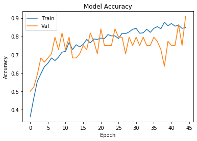
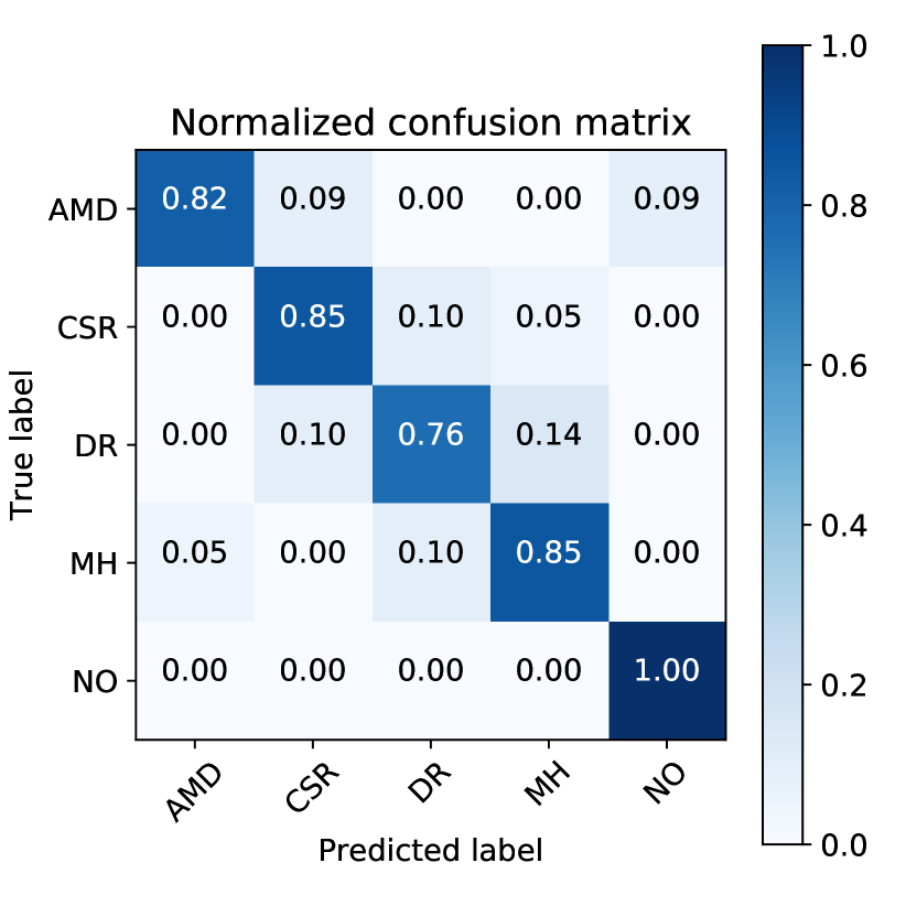
Figure 1: The metrics of the original model - (left) evolution of training and validation accuracy during training, (right) confusion matrix for the test set

2.3 Uncertainty evaluation and explanation

Some of the model weights were removed randomly using the 4 dropout layers at the test time to approximate a Bayesian neural network. The 10^th percentile level from the training set was used to generate thresholds for each class in the initial analysis. The test samples with uncertainty higher than the threshold (lower probability of prediction) were marked as referrals for manual diagnosis by an expert.

The explanations were produced using an attribution method called DeepTaylor [24]. It was the best performing attribution method from a previous comparative study [13]. It finds a root point near a given neuron with a value close to the input but output as 0. Taylor decomposition is then recursively applied from the output to the input layer to estimate the attributions of each neuron. The Innvestigate library [25] was used to implement the attribution method.

3 Results

A threshold was computed using the 10th percentile of the uncertainty in the training set for each class. These values varied across the classes - amd 0.65, csr 0.92, dr 0.93, mh 0.97, and normal 0.93. The lower threshold for amd indicates a wider spread in uncertainty levels and the presence of false negatives. The thresholds were used to remove 27 of 113 test images and the model accuracy improved from 88.5% to 93.7% for the remaining samples. These improvements for each class are shown by metrics in Table 2 and the new confusion matrix is shown Figure 2.

dr, which had the worst performance originally as shown in Figure 1 (right), showed the largest improvement from 0.76 to 0.92 at the cost of separating 6/21 images for referral. In contrast, only one normal image was sent for referral and zero false positives were maintained. Interestingly, all the false negatives were also eliminated by referring 4/13 amd images. The fraction of correct classifications also increased for the other three classes - 0.82 to 0.89 for amd, 0.85 to 0.88 for csr, and 0.88 for mh. It is apparent from this case that the largest improvements were made in the classes with weakest performance, but no conclusions can be reached without an analysis involving larger and more diverse datasets.

Table 2: Effect of threshold on precision (PR), recall (RE), F1 score and support samples

	Base metrics				After uncertainty
Condition	PR	RE	F1	Support	PR	RE	F1	Support
AMD	0.90	0.82	0.86	11	0.89	0.89	0.89	9
CSR	0.85	0.85	0.85	20	0.88	0.94	0.91	16
DR	0.80	0.76	0.78	21	0.92	0.80	0.86	15
MH	0.81	0.85	0.83	20	0.88	0.93	0.90	15
Normal	0.95	0.95	0.95	41	1.00	1.00	1.00	40

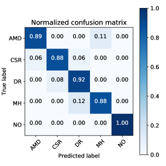
Figure 2: Confusion matrix for the test set after uncertainty threshold

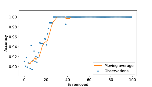
Figure 3: The effect of removing the samples with most uncertainty on the accuracy. The points in the scatter are the observations and the 5 sample moving average shows the overall trend.

Probability distributions of the output were generated by activating random dropout at the test time and repeating for 1000 times for the entire dataset. These probability distribution histograms approximating the Bayesian uncertainty and the corresponding oct images with heatmaps using Deep Taylor are shown for some typical samples in Figure 6. The brighter the color on a given part of the image, the greater the contribution to the model output. The original oct images are also provided for reference. The threshold is plotted as a solid green and the medians of each class are shown by dotted lines. If the class median is below the threshold level, the image should be sent for a referral. The observed relationship between the explanations, uncertainty levels and the model predictions is discussed in section 4.

An analysis performed by removing the test samples with most uncertainty and observing the effect on the model accuracy is plotted in Figure 3. The samples were ordered by the median value of the uncertainty and removed one by one. Small sample size of 113 makes the overall trend noisy and hence moving average analysis with window size 5 was used for smoothing. Almost all the incorrectly classified images were in the initial quarter of uncertainty scores. The moving average has a shape similar to the logistic growth as it reaches 100% accuracy level. In practice, such a graph could be used to set a tolerance level and images below the level can be referred to clinician for diagnosis by a human expert. In further studies with larger datasets, this could be used to produce class wise thresholds from the test set.

4 Discussion

The black-box nature of deep learning models affects their acceptance in practical settings such as healthcare. A clinician is supposed to present the reasoning for decisions. Humans also associate a degree of certainty to their decisions. This is in contrast to the opaqueness of advanced artificial intelligence methods such as deep learning which are hard to understand due to millions of features and give the result as a single class. This study presented an uncertainty aware and explainable deep learning model for retinal diagnosis. The heatmaps using Deep Taylor and the uncertainty using probability histograms supplement the model decision. The end-user can infer the regions the model looked at as well as how sure the model is about the predictions and make a final decision. Also, separating the cases with more uncertainty for referral could help improve model performance and inculcate trust. The improved confusion matrix and accuracy in Figures 2 and 3 respectively indicate the efficacy of uncertainty information. Referring uncertain images to a clinician instead of misdiagnosing can improve patient care by increasing the confidence in the underlying system.

Previous studies [12, 13] compared the heatmaps of each explainability method for a given sample and concluded that Deep Taylor performed the best for retinal oct. There are also studies showing the effect of uncertainty for diagnosis from retinal fundus images [17]. The present study is one of the first to report both the explanations and uncertainty analysis. It is observed that the samples classified with higher certainty also have more relevant heatmaps. Some examples covering all 5 classes and some typical cases are shown in Figure 6. A greater emphasis is laid on the ability to identify model errors using uncertainty and explanations. Figure 5(a) shows the retinal oct of a normal eye for reference.

The model is observed to be the most sensitive to high contrast regions, i.e. the inner retina or the vitreous - retinal interface and the photoreceptor layer. Figure 5(b) shows a correctly classified amd scan where the model showed certainty higher than the corresponding threshold. The model correctly picks up the relevant deposits and new blood vessels in the photoreceptor layer. Figures 5(c) - 6(a) show correctly classified CSR, DR and MH cases.

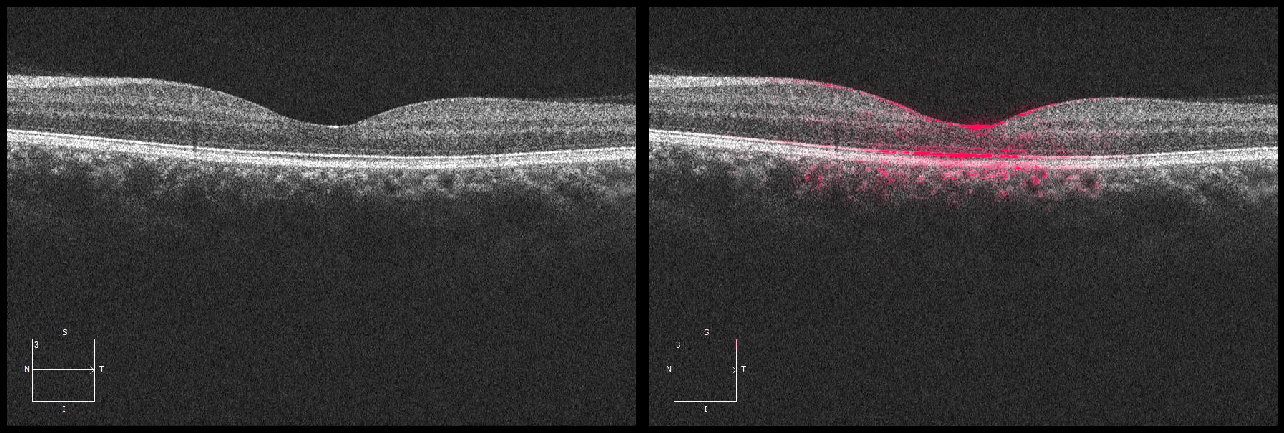
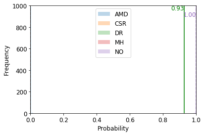
(a) A correctly classified normal image with high certainty. The probability was close to 1 for all the runs. The heatmaps focus on the normal shapes of inner retina and the photoreceptor layer.

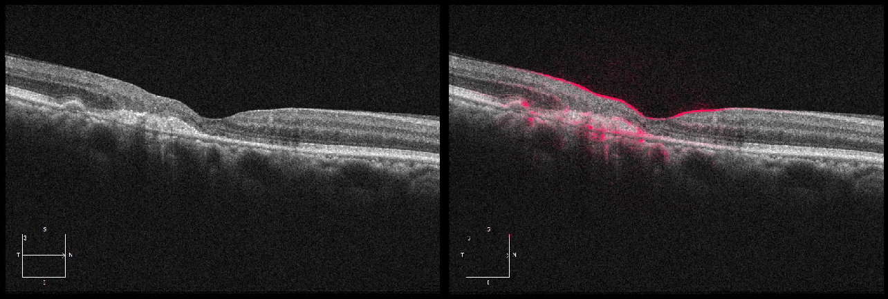
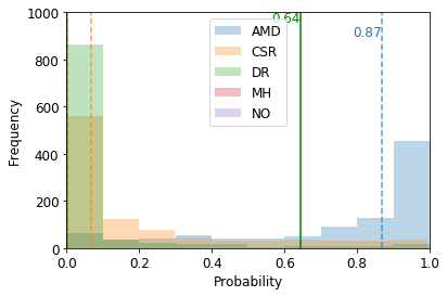
(b) An amd image correctly classified with probability higher than the threshold. The explanations highlight the anomalous photoreceptor layer in the macula.

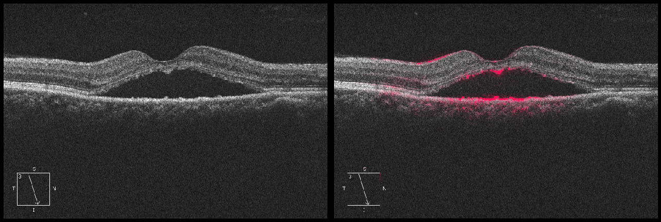
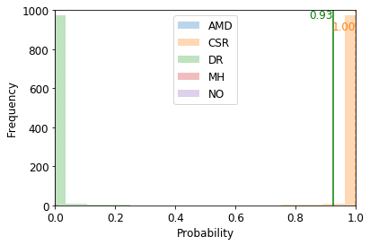
(c) A csr image with prominent features correctly classified with complete certainty.

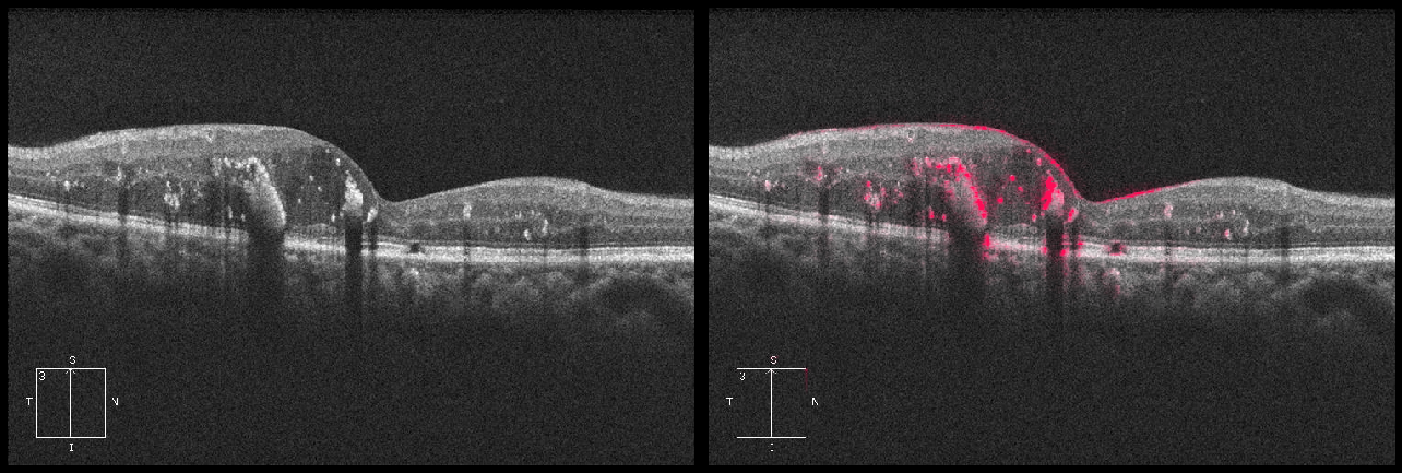
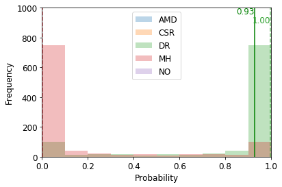
(d) A correctly classified dr image with high certainty. The model detected new blood vessels visible as bright structures with shadows underneath.

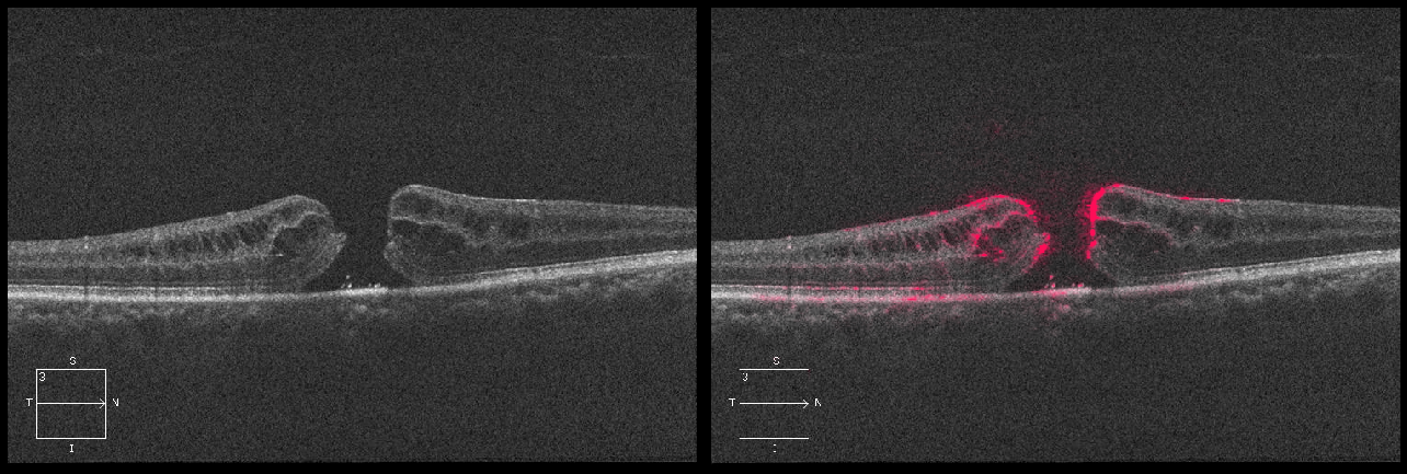
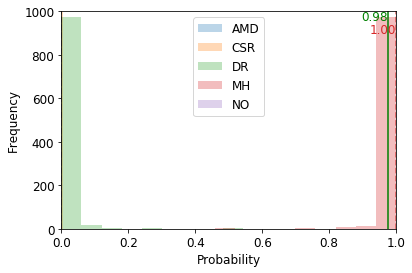
(a) A correctly classified mh image. The certainty is high and the model looked the curved boundaries of the hole.

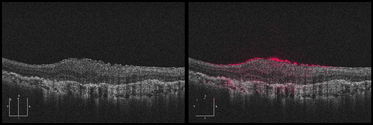
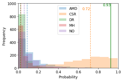
(b) A noisy amd image misclassified as csr with certainty lower than the threshold. Hence, model refers it to a clinician for further diagnosis.

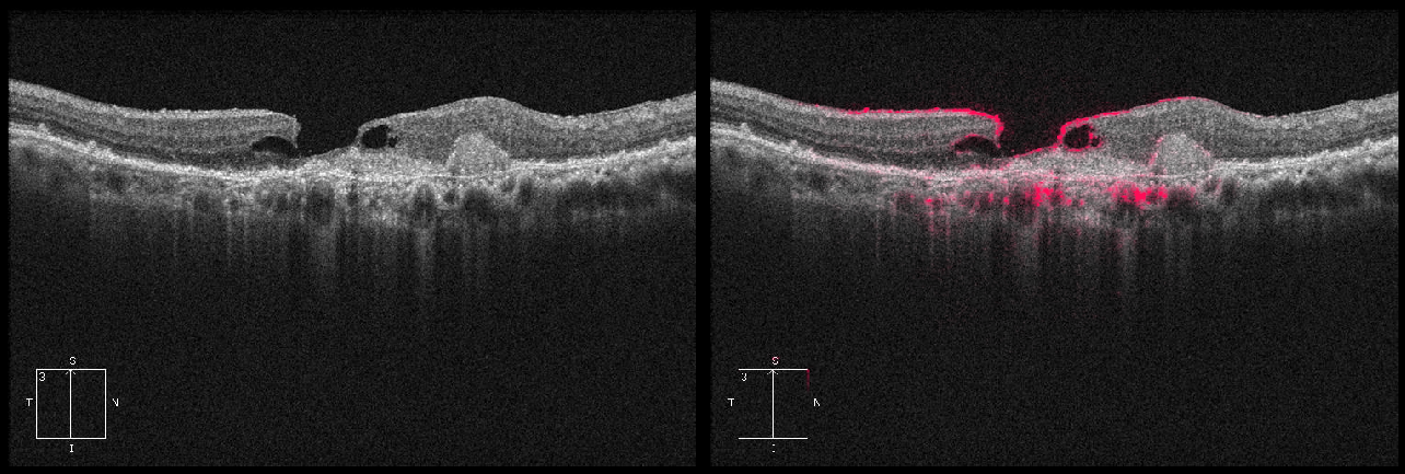
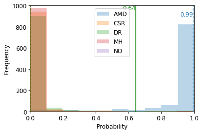
(c) An image labelled as mh in the dataset with both mh and amd classified as amd with high certainty.

Figure 6: (Left to right) The input OCT images, explanations using Deep Taylor and Bayesian uncertainty histograms. The brighter magenta regions had more effect on the output. The histograms shows the distribution of softmax outputs for 1000 runs of the model with medians as dotted and threshold in solid green.

A typical example of csr is shown in Figure 5(c) with as large fluid deposit in the central part of the eye. The model looked at the boundaries of the deposit and correctly classified it with high certainty. Similarly, Figure 5(d) shows a dr which is also classified correctly with high certainty. The model looked at the irregular structures, possibly blood clots or scars in the central retina. The abnormalities in the periphery are not highlighted in most cases. A correctly classified and highly certain mh case is shown in Figure 6(a) where the model mainly looked at the main clinical feature - the boundaries of the hole. Figure 6(b) is a high noise image with diffuse photoreceptor layer. The model emphasized the curvature of the retina while focusing less on the telltale fluid deposits whose boundaries are highlighted in a light magenta. Consequently, mh received the highest probability. The higher threshold of mh ensured the case is sent for a referral instead of misdiagnosing it. Figure 6(c) shows an image which has a clear mh and a possible wet amd. It was labeled as mh in the dataset and the model classified it as amd. It put emphasis on the macular deposits compared to the relatively smaller structure of the hole, thus predicting the secondary diagnosis.

Some general observations can also be drawn about the relationship between uncertainty and the features highlighted by explanations. The cases with higher contrast between the structures seem to be classified with higher certainty. The model looked at the sharp transitions between layers such as the vitreous - retinal and the photoreceptors along with some bright deposits as in Figure 5(d). Clinicians also consider the darker regions such as the fluid accumulations in Figure 5(c) and the shadows of new blood vessels in Figure 5(d). Overall, there is a relationship between the uncertainty, explanations, and the accuracy of a deep learning model for retinal oct images. This study is an initial exploratory analysis and leads to several areas of further research.

5 Conclusion

In this study, the Bayesian uncertainty and the explanations of a deep learning model for retinal diagnosis are demonstrated. It is shown that the threshold with uncertainty successfully improved the model performance by leaving out a few uncertain samples. The effect of removing uncertain samples on the accuracy follows a trend similar to the logistic curve. The uncertainty and the correctness of a decision are related to the explanations. In cases with higher certainty and correct decisions the explanations highlighted the clinically relevant regions the best. Using both uncertainty and explainability has implications in the acceptance of deep learning models. Both the clinical community and AI researchers stand to benefit from this, the former with more holistic information and the latter with a tool to improve models.

Future studies can expand this approach to more domains for improving the deep learning models for real-world applications. This information can be used to alter the features learned by a model and hence improving the robustness. Another direction could be to quantify pathological features such as the brightness and thickness of the retinal pigment epithelium and relate them to the explanations and uncertainty. Designing an uncertainty-aware and explainable system would alleviate the major barriers for acceptance of deep learning methods in multiple domains including medical diagnosis.

References

- [1] De Fauw, J., Ledsam, J. R., Romera-Paredes, B., Nikolov, S., Tomasev, N., Blackwell, S., Askham, H., Glorot, X., O’Donoghue, B., Visentin, D., and Others, “Clinically applicable deep learning for diagnosis and referral in retinal disease,” Nature medicine 24(9), 1342–1350 (2018).
- [2] Sengupta, S., Singh, A., Leopold, H. A., Gulati, T., and Lakshminarayanan, V., “Ophthalmic diagnosis using deep learning with fundus images – A critical review,” Artificial Intelligence in Medicine 102, 101758 (2020).
- [3] Leopold, H. A., Singh, A., Sengupta, S., Zelek, J. S., and Lakshminarayanan, V., [Recent Advances in Deep Learning Applications for Retinal Diagnosis using OCT ], Elsevier, NY, in press (2021).
- [4] Tomsett, R., Preece, A., Braines, D., Cerutti, F., Chakraborty, S., Srivastava, M., Pearson, G., and Kaplan, L., “Rapid Trust Calibration through Interpretable and Uncertainty-Aware AI,” Patterns 1(4), 100049 (2020).
- [5] Singh, A., Sengupta, S., and Lakshminarayanan, V., “Explainable deep learning models in medical image analysis,” Journal of Imaging 6(6), 52 (2020).
- [6] Holzinger, A., Biemann, C., Pattichis, C. S., and Kell, D. B., “What do we need to build explainable AI systems for the medical domain?,” arXiv preprint arXiv:1712.09923 (2017).
- [7] Arrieta, A. B., D′iaz-Rodr′iguez, N., Del Ser, J., Bennetot, A., Tabik, S., Barbado, A., Garc′ia, S., Gil-López, S., Molina, D., Benjamins, R., and Others, “Explainable Artificial Intelligence (XAI): Concepts, taxonomies, opportunities and challenges toward responsible AI,” Information Fusion 58, 82–115 (2020).
- [8] Arya, V., Bellamy, R. K., Chen, P.-Y., Dhurandhar, A., and Hind, M. e. a., “One explanation does not fit all: A toolkit and taxonomy of ai explainability techniques,” arXiv preprint arXiv:1909.03012 (2019).
- [9] Yang, H.-L., Kim, J. J., Kim, J. H., Kang, Y. K., and et. al. Park, D. H., “Weakly supervised lesion localization for age-related macular degeneration detection using optical coherence tomography images,” PloS One 14(4), e0215076 (2019).
- [10] Sayres, R., Taly, A., Rahimy, E., Blumer, K., and et. al. Coz, D., “Using a deep learning algorithm and integrated gradients explanation to assist grading for diabetic retinopathy,” Ophthalmology 126(4), 552–564 (2019).
- [11] Kaur, H., Nori, H., Jenkins, S., Caruana, R., Wallach, H., and Wortman Vaughan, J., “Interpreting Interpretability: Understanding Data Scientists’ Use of Interpretability Tools for Machine Learning,” in [Proceedings of the 2020 CHI Conference on Human Factors in Computing Systems ], 1–14 (2020).
- [12] Singh, A., Sengupta, S., Abdul Rasheed, M., Zelek, J., and Lakshminarayanan, V., “Interpretation of deep learning using attributions : application to ophthalmic diagnosis,” in [In Proc. Applications of Machine Learning, SPIE ], 11511, 115110A, International Society for Optics and Photonics (SPIE) (2020).
- [13] Singh, A., Sengupta, S., Mohammed, A. R., Faruq, I., Jayakumar, V., Zelek, J., Lakshminarayanan, V., et al., “What is the optimal attribution method for explainable ophthalmic disease classification?,” in [International Workshop on Ophthalmic Medical Image Analysis ], 21–31, Springer (2020).
- [14] Chen, H., Lundberg, S., and Lee, S.-I., “Explaining Models by Propagating Shapley Values of Local Components,” arXiv preprint arXiv:1911.11888 (2019).
- [15] Kendall, A. and Gal, Y., “What uncertainties do we need in bayesian deep learning for computer vision?,” in [Advances in neural information processing systems ], 5574–5584 (2017).
- [16] Gal, Y. and Ghahramani, Z., “Dropout as a bayesian approximation: Representing model uncertainty in deep learning,” in [International Conference on machine learning ], 1050–1059 (2016).
- [17] Leibig, C., Allken, V., Ayhan, M. S., Berens, P., and Wahl, S., “Leveraging uncertainty information from deep neural networks for disease detection,” Scientific reports 7(1), 1–14 (2017).
- [18] Pan, H., Wang, Z., Zhan, W., and Tomizuka, M., “Towards better performance and more explainable uncertainty for 3d object detection of autonomous vehicles,” in [2020 IEEE 23rd International Conference on Intelligent Transportation Systems (ITSC) ], 1–7, IEEE (2020).
- [19] Tan, Q., Ye, M., Ma, A. J., Yang, B., Yip, T. C.-F., Wong, G. L.-H., and Yuen, P. C., “Explainable uncertainty-aware convolutional recurrent neural network for irregular medical time series,” IEEE Transactions on Neural Networks and Learning Systems , 1–15 (2020).
- [20] Wickstrøm, K., Kampffmeyer, M., and Jenssen, R., “Uncertainty and interpretability in convolutional neural networks for semantic segmentation of colorectal polyps,” Medical Image Analysis 60, 101619 (2020).
- [21] Gholami, P., Roy, P., Parthasarathy, M. K., and Lakshminarayanan, V., “OCTID: Optical coherence tomography image database,” Computers & Electrical Engineering 81, 106532 (2020).
- [22] Kermany, D. and Goldbaum, M., “Labeled optical coherence tomography (OCT) and Chest X-Ray images for classification,” Mendeley Data 2 (2018).
- [23] Singh, A., Sengupta, S., and Lakshminarayanan, V., “Glaucoma diagnosis using transfer learning methods,” in [In Proc. Applications of Machine Learning, SPIE ], 11139, 111390U, International Society for Optics and Photonics (SPIE) (2019).
- [24] Montavon, G., Lapuschkin, S., Binder, A., Samek, W., and Müller, K.-R., “Explaining nonlinear classification decisions with deep taylor decomposition,” Pattern Recognition 65, 211–222 (2017).
- [25] Alber, M., Lapuschkin, S., Seegerer, P., Hägele, M., and et. al. Schütt, K. T., “iNNvestigate neural networks,” Journal of Machine Learning Research 20(93), 1–8 (2019).