Topological transitivity implies chaos for two-dimensional Filippov Systems

Abstract.

In this work we consider Filippov systems on a two-dimensional manifold with finite number of tangency points. We prove that topological transitivity implies chaos if the Filippov system has non-empty sliding or escaping regions. We also prove that in this setting, as it happens for continuous flows, topological transitivity is equivalent to the existence of a $G_{\delta}$ set of transitive points.

1. Introduction

It is widely accepted that ordinary differential equations (ODE) are very accurate for modeling problems emerging from real world applications. Accordingly, a large range of models from physics, engineering, biology, economics, medicine, among others, can be studied by assuming that some distinguished variables of them evolving in time according to some dynamical rule. In the case of ODE such rules are flows associated to some $C^{r}$-vector field and the time is assume to vary continuously. However, in recent decades the assumption that trajectories may experience a discontinuity have gained traction within the theory of dynamical systems.

The presence of discontinuities in ODE modeling concrete phenomena are mainly due to abrupt changes in the dynamics. It may occur, for instance, when certain object suffers an impact or change its motion from frictionless movement to some rough dynamic, the former sometimes refereed as stick-slip process. Another situation that can be modeled in terms of discontinuities are those under the effects of fast switches as occurs in some electronic circuits or relay systems. In such case, the change of the dynamics occurs so fast that it can be assumed to be instantaneous although the movement itself is continuous. A non-exhaustive list of applications of discontinuous ODE, besides the ones described before includes control theory, the dynamics of a bouncing ball and foraging predators, the anti-lock braking system (ABS), mechanical devices in which components collide to each other, problems with friction, sliding or squealing, etc. See the referred applications and others in [2], [3], [4], [6], [8], [10], [11], [12], [13] as well as references therein.

We stress that when considering discontinuous ODEs the solution (i.e. a trajectory) does not present “jumps”, in other words the trajectory itself is not discontinuous, the discontinuity happens in the velocity. In this context what can happen is a non-uniqueness of solution. Therefore, some classical results based on uniqueness of trajectories can easily fail and non typical behavior could emerge. It is interesting to not that the discontinuous ODEs present similarities to the so-called impulsive differential equations (IDE) but in general the results are different since IDEs allow solutions to be discontinuous.

Discontinuous ODE may be treated under distincts points of view as differential inclusions, hybrid systems or into the area of complementarity problems. Even assuming the same scenario, different interpretations of solutions may appear in the literature, maybe the most studied has been the Filippov convention, see [7]. Filippov assume that solutions can slide through the discontinuity region according to some rule involving the systems governing the dynamics around where the switching takes place, see Section 2 to details. We will call ODE with discontinuities Filippov systems as we shall follows Filippov’s convention.

A classical result from continuous flows states that topological transitivity is equivalent to the existence of a $G_{\delta}$ set of transitive points. In order to provide the theory of Filippov systems with a solid theory we address the topological transitivity for Filippov systems in this work. In particular we obtain that the same result holds for two-dimensional manifold. We prove the following:

Theorem 1.1.

Assume that $M$ is a two-dimensional manifold with a Filippov system having a finite number of tangency points. Then, the Filippov system is topologically transitive on $M$ if, and only if, there is a $G_{\delta}$ set of points which admits a dense Filippov orbit through each of these points.

Filippov systems have important sets associated to the discontinuous manifold, namely escaping and sliding region (see §2). We prove that if one of these sets are non-empty and the Filippov system is transitive, then it admits chaotic behavior.

Theorem 1.2.

Assume that $M$ is a two-dimensional manifold with a transitive Filippov system having a finite number of tangency points. If the sliding or escaping regions are non-empty, then the following statements hold:

• There is a $G_{\delta}$ set $\Delta$ such that:

  • if $x\in\Delta$, then there is a dense orbit through $x$ which is dense;

  • if $x\in\Delta$, then the periodic orbits through $x$ form a dense set.

• The Filippov system is sensitive to initial conditions on $M$;

This paper is organized as follows: Section 2 presents the first concepts and definitions of Filippov systems which are going to be used throughout the paper. In Section 3 we prove Theorem 1.2 and the proof of Theorem 1.1 is done in Section 4.

2. Preliminars

Let $M$ be a 2-dimensional $C^{k}$ closed manifold and $\Sigma\subset M$ a set formed by the union of $n$ smooth curves $\Sigma_{i}$ which are disjoint pairwise, where $\Sigma_{i}=h_{i}^{-1}(0)$ with $i=1,\ldots,n$ and $h_{i}:M\longrightarrow\mathbb{R}$ is a smooth function having $0$ as regular value. We write $\Sigma=\bigcup_{i=1}^{n}\Sigma_{i}$ and assume that $\Sigma$ splits $M$ into $n+1$ disjoint regions $R_{i}$, on which we define $n+1$ vector fields $X_{i},\ldots,X_{n+1}$. We call $\Sigma$ the switching manifold and assume that it is contained on the boundary of the regions $R_{i}$.

We call $\chi$ the space of C^r-vector fields $X:M\longrightarrow TM$ with $1\leq r\leq k$ where $k$ is sufficiently large. Call $\Omega$ the space of non-smooth vector fields $Z:M\rightarrow TM$ such that

(1) $$Z(x) = X_{i}(x),\quad\mbox{if}\quad x\in R_{i},\quad i=1,\ldots,n+1$$

$$Z(x) = \frac{Y_{i_{2}}h_{i}(x)Y_{i_{1}}-Y_{i_{1}}h_{i}(x)Y_{i_{2}}}{Y_{i_{2}}h_{i}(x)-Y_{i_{1}}h_{i}(x)}\quad\mbox{if}\quad x\in\Sigma_{i}$$

where $Y_{i_{1}}$ and $Y_{i_{2}}$ are some of the vectors $X_{i}$ where $Y_{i_{1}}$ is the vector field associated to the the positive part of $h_{i}$ and $Y_{i_{2}}$ associated to the negative part of $h_{i}$.

There are five kind of points on $\Sigma$. They can be classified as follows:

• At crossing points both vector fields points to the same side of $\Sigma$, so trajectories reaching such points immediately crosses from one side to another.

• At sliding points vectors fields point in opposite direction but towards $\Sigma$ so that trajectories reach sliding in finite future time.

• At escaping points vectors fields point in opposite direction but now away from $\Sigma$ so that trajectories reach escaping in finite past time.

• At tangency points one of the vector fields is tangent to $\Sigma$ and the other may be tangent or not. In this first case we refer to it as regular tangency and in the second one it is called a double tangency.

• At pseudo equilibrium points the vector fields are linearly dependent pointing toward or away to $\Sigma$ but in opposite directions. At those points trajectories run away from $\Sigma$ for future or past time.

The above set of points are defined respectively as $\Sigma^{e}$, $\Sigma^{s}$, $\Sigma^{e}$, $\Sigma^{t}$ and $\Sigma^{p}$. Some of these points are represented in the picture below.

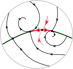
Figure 1. A Filippov system on $S^{2}$. The continuous path between the tangency points are sliding one except by the pseudo equilibrium reached by the two dashed orbits.

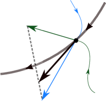
Figure 2. Defining a vector field on the switching manifold.

From equation (1) we note that a non-smooth vector field $Z$ is also defined on points of sliding and escaping type through a convex combination of $Y_{i1}$ and $Y_{i2}$. Those orbits sliding on $\Sigma$ are formed by points on which trajectories collide to it for forward or backward finite time (see Figure 1).

The following definition can be found in [9].

Definition 2.1.

By a Filippov orbit we mean a map $\gamma:\mathbb{R}\rightarrow M$ such that $\gamma$ is a solution of the Filippov system, that is, if $\gamma(t)$ is outside $\Sigma$ then the orbit is locally determined by the vector field, once the orbit touches $\Sigma$ then its orbit is determined by the vector on $\Sigma$ as defined in 1. In the case the orbit goes through a escaping region it may exit at any arbitrary moment.

Definition 2.2.

The saturation of a set $\mathcal{A}$ will be denoted $\mathcal{A}_{\varphi}$, that is, $\mathcal{A}_{\varphi}$ is the union of every Filippov orbit with initial condition on $\mathcal{A}$.

Since we are interested in chaotic aspects of Filippov orbits, we next introduce the definition of chaotic Filippov systems. It is based on the classical definition of Devaney for chaos, see [5].

Definition 2.3.

We define topological transitivity, sensitive dependence on initial conditions and chaoticity for Filippov system 1 as follows:

• $Z$ is topologically transitive on a set $N\subset M$ if given any two open set $U$ and $V$ of $M$, there exist a Filippov orbit which intersects $U$ and $V$.

• $Z$ exhibits sensitive dependence with respect to initial condition if if there is a fixed $r>0$ such that for any open set $U$ there exist $x,y\in U$ and two Filippov systems $\gamma_{x}$ and $\gamma_{y}$ which starts at $x$ and $y$ respectively and such that there is some time $t$ with $d(\gamma_{x}(t),\gamma_{y}(t))>r$.

• A Filippov orbit $\gamma$ is periodic is there is $\tau$ such that $\gamma(t)=\gamma(t+\tau),\;\forall t\in\mathbb{R}$.

• $Z$ is chaotic if it is topologically transitive, has sensitive dependence with respect to initial condition and the union of all Filippov periodic orbits form a dense set.

3. Proof of Theorem 1.2

Proof.

We shall proof a number of interesting lemmas that will be needed for the proof of our result. We first prove the theorem for the case the sliding region is non-empty (i.e. $\Sigma^{s}\neq\emptyset$).

Lemma 3.1.

Assume topological transitivity and $M^{s}\neq\emptyset$. Then $int(M^{s}_{\varphi})\neq\emptyset$ and $M^{s}_{\varphi}$ is dense in $M$.

Proof.

First note that the interior of $M^{s}_{\varphi}$ is not empty because both sliding and escaping regions always have a segment that saturated has non empty interior, see Figure 3.. To prove the second statement, note that if $M^{s}_{\varphi}$ is not dense, then the interior of $(M^{s}_{\varphi})^{c}$ is not empty. Now consider open sets $\mathcal{U}\subset int(M^{s}_{\varphi})$ and $\mathcal{V}\subset int[(M^{s}_{\varphi})^{c}]$. By topological transitivity there is a Filippov orbit from $\mathcal{U}$ to $\mathcal{V}$, which is an absurd since these two sets are inside disjoint invariant ones. ∎

\begin{overpic}[width=199.16928pt]{saturacao_sliding_escape.eps} \put(15.0,12.0){$a_{i}$}\put(4.0,18.0){$V_{i}$} \put(75.0,28.0){$b_{i}$}\put(82.0,32.0){$W_{i}$} \end{overpic}

Figure 3.

Lemma 3.2.

Assume that $M^{s}\neq\emptyset$ and more precisely that $\Sigma^{s}\neq\emptyset$. Then there is a dense set $\{a_{i}\}_{i\in\mathbb{N}}$ of $M$ such that $\{a_{i}\}_{i\in\mathbb{N}}\subset M^{s}_{\varphi}$ and open sets $V_{i}\subset M^{s}_{\varphi}$ containing $a_{i}$ such $V_{i}$ flows into the sliding region as illustrated by Figure 3.

Proof.

Let $W\subset M^{s}_{\varphi}$ be the set of points whose first loss of positive uniqueness occurs on a tangency point. That is if $x\in W$, then there exists a Filippov orbit $\gamma$ such that $\gamma(t_{0})=x$ and $\gamma(t)$ for $t\in[0,t_{0})$ do not contain tangency points, sliding or escaping points. Notice that this set is a meager set since $M$ has a finite number of tangency points.

Therefore, $W^{c}$ is a $G_{\delta}$ set. By the construction of $W^{c}$, notice that the possible choice for the Filippov orbit starting on a point of it is one of the following: either it looses the uniqueness after entering the sliding region $\Sigma^{s}$, call this set $A$, or it does not loose uniqueness, call this set $B$. Notice that by Lemma 3.1 we get $int(B)=\emptyset$.

Given $x\in W^{c}$ and an open set $\mathcal{U}_{x}\subset M$ containing $x$ there is a point $a\in A$ such that $a\in\mathcal{U}_{x}$. But because the first break of uniqueness of $a$ is entering a sliding we can consider an open set $\mathcal{U}_{a}\subset\mathcal{U}_{x}$ such that all points of $\mathcal{U}_{a}$ loose uniqueness of trajectory entering the sliding $\Sigma^{s}$. Hence consider a dense countable number of point $a_{i}\in W^{c}$. We obtain from the previous method an open set $\mathcal{V}_{a_{i}}=:V_{i}$ with the desirable property. ∎

For the next two lemmas we shall consider the additional hypothesis that $\Sigma^{s}\neq\emptyset$, also in this case we fix a point $q_{0}\in\Sigma^{s}$ and $\mathcal{U}$ an open set with the following property: if $q\in\mathcal{U}$ then the orbit starting from $q$ will touch $q_{0}$ as shown in Figure 5.

\begin{overpic}[width=165.02606pt]{sliding.eps} \put(24.0,41.0){$q_{0}$}\put(16.0,43.0){$U$} \put(71.0,19.0){$q^{\prime}$}\put(87.0,19.0){$q$} \put(-8.0,24.0){$\Sigma^{s}$} \end{overpic}

Figure 4.

\begin{overpic}[width=165.02606pt]{escaping.eps} \put(58.0,17.0){$T_{0}$} \put(-9.0,23.0){$\Sigma^{e}$} \end{overpic}

Figure 5.

Lemma 3.3.

Assume topological transitivity and $\Sigma^{s}\neq\emptyset$. Given any point $q\in\Sigma^{s}$, then there is a Filippov orbit segment from $q_{0}$ to $q$.

Proof.

Let $q^{\prime}\in\Sigma^{s}$ be a point close to $q$ such that the positive orbit from $q^{\prime}$ has to touch $q$ similar to what was done above, see Figure 5. Now let $\mathcal{U}^{\prime}$ be a neighborhood of $q^{\prime}$ small enough so that it does not intersect $q$ and such that every point in $\mathcal{U}^{\prime}$ the forward trajectory has to intersect $q$. By topological transitivity there is an orbit from $\mathcal{U}$ to $\mathcal{U}^{\prime}$ and by our choices of $\mathcal{U}$ and $\mathcal{U}^{\prime}$ there is a trajectory from $q_{0}$ to $q$. ∎

Lemma 3.4.

Assume topological transitivity and $\Sigma^{s}\neq\emptyset$, then there is a Filippov orbit segments $\gamma_{i}:[0,t_{i}]\rightarrow M$ such that $q_{0}=\gamma_{i}(0)=\gamma_{i}(t_{i})$ and $\gamma_{i}([0,t_{i}])\cap V_{i}\neq\emptyset$ where $t_{i}>0$ for all $i=0,1,2,\ldots$ and $V_{i}$ as in Lemma 3.2.

Proof.

By topological positive transitivity there is an orbit from $\mathcal{U}$ to $\mathcal{V}_{i}$ and by the choice of $\mathcal{U}$ it means that this orbit passes through $q_{0}$, but Lemma 3.2 implies that this orbits goes to a sliding piece and from Lemma 3.3 this orbit reaches point $q_{0}$, so the result is proved. ∎

For the proof assuming that the escaping region is non-empty is a very similar argument which we point out briefly.

Lemma 3.5.

Assume that $M^{s}\neq\emptyset$ and more precisely that $\Sigma^{e}\neq\emptyset$. Then there is a dense set $\{b_{i}\}_{i\in\mathbb{N}}$ of $M$ such that $\{b_{i}\}_{i\in\mathbb{N}}\subset M^{s}_{\varphi}$ and open sets $W_{i}\subset M^{s}_{\varphi}$ containing $b_{i}$ such $W_{i}$ flows through backward time into the escaping region as illustrated by Figure 3.

Proof.

The proof follows the similar ideas as in the proof of Lemma 3.2. Consider the meager sets of points which touches the tangency points for the first time in backwards time and after construct the sets $W_{i}$ in the same manner as $V_{i}$. ∎

We now fix a point $T_{0}$ which is a tangency point for a sliding region, in particular we assume that a point entering the escaping region which $T_{0}$ belongs has to enter though $T_{0}$, see Figure 5.

Lemma 3.6.

Assume topological transitivity and $\Sigma^{e}\neq\emptyset$. Given any point $q\in\Sigma^{u}$, then there is a Filippov orbit segment from $T_{0}$ to $q$.

Proof.

As observed before, to enter a escaping region one has to go through a tangency. Consider a set $W_{i}$ and $W_{j}$ with the properties as in Lemma 3.5 such that $W_{0}$ is associated to the escaping region of $T_{0}$ and $W_{j}$ associated to the escaping region of $p$ then topological transitivity implies these two set are connected but for that the orbit has to enter both escaping region one can now easily fine an orbit connecting both point $T_{0}$ and $q$. ∎

Lemma 3.7.

Assume $\Sigma^{e}\neq\emptyset$, then there is a Filippov orbit segments $\gamma_{i}:[0,t_{i}]\rightarrow M$ such that $T_{0}=\gamma_{i}(0)=\gamma_{i}(t_{i})$ and $\gamma_{i}([0,t_{i}])\cap W_{i}\neq\emptyset$ where $t_{i}>0$ for all $i=0,1,2,\ldots$ and $W_{i}$ as in Lemma 3.5.

Proof.

Let $W_{0}$ the open set associated to $T_{0}$ with the properties as in Lemma 3.5. Now given $W_{i}$ by topological transitivity there is a Filippov curve which connects $W_{i}$ to $W_{0}$ and since we can connect $T_{0}$ to any point in a escaping region we close a curve by going from $T_{0}$ to the tangency point that is the entrance of the associated escaping region of $W_{i}$ and leave this escaping in order to go through $W_{i}$ and back to $W_{0}$ by is one goes back to $W_{0}$ has to have entered through $T_{0}$ and when that happens we get the periodic segment as wanted. ∎

The proof of the theorem is completed with the above lemmas. ∎

4. Proof of Theorem 1.1

Proof.

If $M^{s}\neq\emptyset$, then the result follows from Theorem 1.2. The case $M^{s}=\emptyset$ will follow from the two lemmas below. We now assume that the Filippov systems is topologically transitive, since the converse is trivial.

Lemma 4.1.

Assume topological transitivity, $M^{s}=\emptyset$ and $\Sigma^{t}_{\varphi}$ is dense. Then there is a $G_{\delta}$ set of $M$ such that each point in this set has some dense Filippov orbit.

Proof.

Now, recall that we are assuming a finite number of tangency points and our space is two dimensional. Hence, we may construct a Filippov orbit inside $\Sigma^{t}_{\varphi}$ which is dense.

Let us call this dense Filippov orbit as $\gamma(t)$ and let $t_{0}$ the time such that $\gamma(t_{0})\in\Sigma^{t}$ and $\gamma(t)\cap\Sigma^{t}=\emptyset$ for all $t>t_{0}$. Therefore $\gamma([t_{0},\infty])$ is dense in $M$ and it does not intersect any tangency point.

Let $g:M\rightarrow[0,1]$ be a smooth function such that $g^{-1}(0)=\Sigma^{t}$. Now let us change the velocity of the Filippov orbit associated to the vector field of system by multiplying it by the positive map $g$. Hence the new vector field $gZ$ is in fact a continuous vector field whose orbits coincide to the previous one, with the exception that now the tangency points are fixed ones. But now this new Filippov system is in fact a continuous flow, and for this new flow, $\gamma[t_{0},\infty]$ is the image of some trajectory of it (which is dense).

Hence, in particular because there is a dense orbit for a continuous flows we guarantee from classical results of continuous flows that there is a $G_{\delta}$ set $D$ of points with dense orbit. Notice that none of this dense orbits can pass through the singular points of $gZ$, hence these are also dense orbits for the Filippov system.

Notice that $\Sigma^{t}_{\varphi}$ is a meager set, hence $D\backslash\Sigma^{t}_{\varphi}$ is a $G_{\delta}$ set and the image of the orbit of these points for the flow $gZ$ is the same as for the original Filippov system. ∎

Lemma 4.2.

Assume topological transitivity, $M^{s}=\emptyset$ and $\Sigma^{t}_{\varphi}$ is not dense. Then there is a $G_{\delta}$ set of $M$ such that each point in this set has some dense orbit. Moreover, these dense orbits are regular orbits.

Proof.

If $\Sigma^{t}_{\varphi}$ is not dense, then the interior of its complement $\left(\Sigma^{t}_{\varphi}\right)^{c}$ is nonempty. Let us take $\mathcal{U}\subset int[\left(\Sigma^{t}_{\varphi}\right)^{c}]=:A$. Now we prove that $A$ is dense. Indeed, given an open set $\mathcal{V}\subset M$, from the topological transitivity of the Filippov system there is a point $x\in\mathcal{V}$ and an orbit from $x$ to $\mathcal{U}$ which is a regular since it outside the set where the break of uniqueness occurs. Hence there is an open set $\mathcal{V}_{0}\subset V$ containing $x$ such that every segment of orbit from $\mathcal{V}_{0}$ to $\mathcal{U}$ is regular, which is true for $\mathcal{V}_{0}$ sufficiently small. Therefore from the invariance of the set $A$, we get that $\mathcal{V}_{0}\subset A$. That means the Filippov system on $A$ is topologically transitive, but on this invariant set $A$ the Filippov system determines a continuous flow since $A\cap\Sigma\subset\Sigma^{c}$ because $M^{s}=\emptyset$. Thus there is a $G_{\delta}$ set of points whose orbit is dense in $A$.

The lemma is proved, since $Z$ on $A$ is a continuous flows, $A$ is an open and dense set and $Z$ restricted to $A$ has a dense orbit. ∎

The above lemmas prove the result. ∎

Acknowledgments. The authors would like to thank Professor Marco A. Teixeira for useful conversations concerning this work. R.E. is partially supported by Pronex/ FAPEG/CNPq grant 2012 10 26 7000 803 and grant 2017 10 26 7000 508, Capes grant 88881.068462/2014-01 and Universal/CNPq grant 420858/2016-4. R.V. was partially supported by FAPESP (grant # 2016/22475-9), by the Coordenação de Aperfeiçoamento de Pessoal de Nível Superior - Brasil (CAPES) - Finance Code 001 and by CNPq.

References

- [1] M. di Bernardo, A. Colombo and E. Fossas, Two-fold singularity in nonsmooth electrical systems, Proc. IEEE International Symposium on Circuits ans Systems, (2011), 2713–2716.
- [2] M. di Bernardo, K.H. Johansson, and F. Vasca, Self-Oscillations and Sliding in Relay Feedback Systems: Symmetry and Bifurcations, Internat. J. Bif. Chaos, vol. 11, (2001), pp. 1121-1140.
- [3] B. Brogliato, Nonsmooth Mechanics: Models, Dynamics and Control, Springer- Verlag, New York, 1999.
- [4] F. Dercole and F.D. Rossa, Generic and Generalized Boundary Operating Points in Piecewise-Linear (discontinuous) Control Systems, In 51st IEEE Conference on Decision and Control, 10-13 Dec. 2012, Maui, HI, USA. Pages:7714-7719. DOI: 10.1109/CDC.2012.6425950.
- [5] Devaney, Robert L. An introduction to chaotic dynamical systems, Studies in Nonlinearity. Westview Press, Boulder, CO, 2003.
- [6] D.D. Dixon, Piecewise Deterministic Dynamics from the Application of Noise to Singular Equation of Motion, J. Phys A: Math. Gen. 28, (1995), 5539-5551.
- [7] A.F. Filippov, Differential Equations with Discontinuous Righthand Sides, Mathematics and its Applications (Soviet Series), Kluwer Academic Publishers-Dordrecht, 1988.
- [8] S. Genena, D.J. Pagano and P. Kowalczik, Hosm Control of Stick-Slip Oscillations in Oil Well Drill-Strings, In Proceedings of the European Control Conference 2007 - ECC07, Kos, Greece, July.
- [9] M. Guardia, T.M. Seara and M.A. Teixeira, Generic bifurcations of low codimension of planar Filippov Systems, Journal of Differential Equations 250 (2011) 1967–2023.
- [10] A. Jacquemard and D.J. Tonon, Coupled systems of non-smooth differential equations, Bulletin des Sciences Mathématiques, vol. 136, (2012), pp. 239-255.
- [11] T. Kousaka, T. Kido, T. Ueta, H. Kawakami and M. Abe, Analysis of Border- Collision Bifurcation in a Simple Circuit, Proceedings of the International Symposium on Circuits and Systems, II-481-II-484, (2000).
- [12] R. Leine and H. Nijmeijer, Dynamics and Bifurcations of Non-Smooth Mechanical Systems, Lecture Notes in Applied and Computational Mechanics, vol. 18, Berlin Heidelberg New-York, Springer-Verlag, (2004).
- [13] M. di Bernardo, C.J. Budd, A.R. Champneys and P. Kowalczyk, Piecewise-smooth Dynamical Systems Theory and Applications, Springer-Verlag (2008).