Multigrid as an exact solver

Abstract

We provide an alternative Fourier analysis for multigrid applied to the Poisson problem in 1D, based on explicit derivation of spectra of the iteration matrix. The new Fourier analysis has advantages over the existing one. It is easy to understand and enables us to write the error equation in terms of the eigenvector of the stiffness matrix. When weighted-Jacobi is used as a smoother with two different weights, multigrid is an exact solver.

1 Introduction

We consider the Poisson problem with Dirichlet boundary conditions given by

$$\left\{\begin{array}[]{ll}-u^{\prime\prime}(x)=f(x),\qquad 0<x<1,\\ u(0)=u(1)=0.\end{array}\right.$$ (3)

The domain of the problem is partitioned into $n-1$ uniform subintervals using the grid points $x_{j}=jh$ where $h=1/(n-1)$ is the grid size, and $n$ is an odd integer. Discretization of the Poisson problem (3) with central finite difference scheme gives the linear systems of equations,

$$A\mathbf{u}=\mathbf{f}$$

where $A=1/h^{2}\text{tridiag}\left(-1,2,-1\right)\in\mathbb{R}^{(n-2)\times(n-2)}$. The matrix $A$ assumes the eigenvectors $\mathbf{v}_{k}^{j}=\sin\left(\frac{jk\pi}{n-1}\right)$ with the corresponding eigenvalues $\lambda_{k}(A)=\frac{4}{h^{2}}\sin^{2}\left(\frac{k\pi}{2(n-1)}\right)$ for $k=1,...,n-2$. Note that $\mathbf{v}_{k}^{j}$ represent the $j-$th entry of the eigenvector $\mathbf{v}_{k}$.

2 Smoother

We use wieghted-Jacobi relaxation as a smoother. Let $a_{i,j}$, $i,j=1,...,n-2$, represent the entries of $A$. We split the matrix $A$ as follows.

$$A=D+K$$

where $D$ is the diagonal matrix with entries $d_{i,i}=a_{i,i}$, ($i=1,...,n-2$). Weighted-Jacobi is defined as

$$\mathbf{x}^{k+1}=(I-\omega D^{-1}A)\mathbf{x}^{k}+\omega D^{-1}\mathbf{f},$$ (4)

where $\omega$ is the weight to be determined. There is no restriction on $\omega$ because it is not necessary for a smoother to be convergent for a multigrid method to be convergent. Let $R_{j}^{\omega}$ represent the iteration matrix of the weighted-Jacobi given in (4).

$$R_{J}^{\omega}\equiv I-\omega D^{-1}A.$$

We can apply the weighted-Jacobi more than one with different $\omega$’s to further accelerate the convergence. To this end, we use the following notation.

$$S_{J}^{m}\equiv S_{J}(\omega_{1},...,\omega_{m})\equiv R_{J}^{\omega_{1}}....R_{J}^{\omega_{m}},$$

which means that the weighted-Jacobi is applied $m$ times with the parameters $\omega_{i}$, $i=1,...,m$. Note that the matrix $S_{J}^{m}$ assumes the same eigenvectors with the matrix $A$. The best way to find the optimal weights of the weighted-Jacobi method as a smoother, is to do spectral analysis. To this end, we carry out a spectral analysis based on explicit derivation of the spectra of the iteration matrix of the two-grid.

3 Other elements of the multigrid method and derivation of the spectrum of the iteration matrix of the two-grid

In this section, we introduce interpolation and restriction operators and show some equalities related to them which are necessary to obtain the spectrum of the iteration matrix of the two-grid. We start by setting $A=A^{h}$, $\mathbf{u}=\mathbf{u}^{h}$ and $\mathbf{f}=\mathbf{f}^{h}$ where the superscript $h$ which is equivalent to the grid size $h$, stands for the fine grid. The two-grid iteration matrix with only pre-smoothing with damped Jacobi relaxation is given by [2]

$$R^{TG}=(I-I_{2h}^{h}(A^{2h})^{-1}I_{h}^{2h}A^{h})S_{J}^{m}.$$ (5)

Our aim is to find the spectrum of $R^{TG}$. Just for easiness of our analysis, we assumed that $n$ is an odd integer. In Equation (5), the prolongation (interpolation) operator $I_{2h}^{h}$ is the linear interpolation which has the matrix form

$$I_{2h}^{h}=\frac{1}{2}\begin{bmatrix}&1&&&\\ &2&&&\\ &1&1&&\\ &&2&\ddots&\\ &&1&\ddots&\\ &&&&1\\ &&&&2\\ &&&&1\end{bmatrix}\in\mathbb{R}^{(n-2)\times(n-3)/2}$$

and restriction operator $I_{h}^{2h}$ is the transpose of the prolongation operator

$$I_{h}^{2h}=\left(I_{2h}^{h}\right)^{T}.$$

Coarse grid matrix $A^{2h}$ is defined by Galerkin projection

$$A^{2h}=I_{h}^{2h}A^{h}I_{2h}^{h}.$$ (6)

From the above definition, it is easy to show that $A^{2h}$ is also symmetric. We apply only pre-smoothing and do not apply post-smoothing.

The prolongation operator $I_{2h}^{h}$ satisfies

$$I_{2h}^{h}\mathbf{v}_{k}^{2h}=\cos^{2}\left(\frac{k\pi}{2(n-1)}\right)\mathbf{v}_{k}^{h}-\sin^{2}\left(\frac{k\pi}{2(n-1)}\right)\mathbf{v}_{n-1-k}^{h},\qquad 1\leq k\leq\frac{n-3}{2}$$ (7)

where

$$\mathbf{v}_{k,j}^{2h}=\sin\left(\frac{2jk\pi}{n-1}\right),\qquad 1\leq j\leq\frac{n-3}{2}.$$ (8)

The restriction operator $I_{h}^{2h}$ which is the transpose of the prolongation operator has the following properties.

$$I_{h}^{2h}\mathbf{v}_{k}^{h}=2\cos^{2}\left(\frac{k\pi}{2(n-1)}\right)\mathbf{v}_{k}^{2h}\quad\textmd{for}\quad 1\leq k\leq\frac{n-3}{2}$$ (9)

and

$$I_{h}^{2h}\mathbf{v}_{n-1-k}^{h}=-2\sin^{2}\left(\frac{k\pi}{2(n-1)}\right)\mathbf{v}_{k}^{2h}\quad\textmd{for}\quad 1\leq k\leq\frac{n-3}{2}.$$ (10)

As we stated before, the coarse grid matrix is obtained by Galerkin projection. That is,

$$A^{2h}=I_{h}^{2h}A^{h}I_{2h}^{h}.$$

Using this definition and properties of the restriction and prolongation operators in (7), (9) and (10), we obtain the spectrum of the coarse matrix $A^{2h}$.

$$A^{2h}\mathbf{v}_{k}^{2h}=\left(2\lambda_{k}(A^{h})\cos^{4}(k\pi h/2)+2\lambda_{n-1-k}(A^{h})\sin^{4}(k\pi h/2)\right)\mathbf{v}_{k}^{2h},\qquad 1\leq k\leq\frac{n-3}{2}.$$ (11)

From the above observations, it is very reasonable to expect that the eigenvectors of the matrix $R^{TG}$ are linear combinations of $\mathbf{v}_{k}$ and $\mathbf{v}_{n-1-k}$. We assume that $\mathbf{b}_{k}=\mathbf{v}_{k}+c\mathbf{v}_{n-1-k}$ is an eigenvector of the matrix $R^{TG}$ where $c$ is to be determined. Imposing $\mathbf{b}_{k}$ into the definition of $R^{TG}$ in (5) and using the properties of the smoother, prolongation, restriction operators and coarse grid matrix we end up with

$$R^{TG}\mathbf{b}_{k}=\mathbf{v}_{k}\left(\lambda_{k}(S_{j}^{m})-\frac{2\cos^{4}(k\pi h/2)\lambda_{k}(A^{h})\lambda_{k}(S_{j}^{m})}{\lambda_{k}(A^{2h})}+c\frac{2\sin^{2}(k\pi h/2)\cos^{2}(k\pi h/2)\lambda_{n-1-k}(A^{h})\lambda_{n-1-k}(S_{j}^{m})}{\lambda_{k}(A^{2h})}\right)$$

$$+c\mathbf{v}_{n-1-k}\left(\lambda_{n-1-k}(S_{j}^{m})-\frac{2\sin^{4}(k\pi h/2)\lambda_{n-1-k}(A^{h})\lambda_{n-1-k}(S_{j}^{m})}{\lambda_{k}(A^{2h})}+\frac{1}{c}\frac{2\sin^{2}(k\pi h/2)\cos^{2}(k\pi h/2)\lambda_{k}(A^{h})\lambda_{k}(S_{j}^{m})}{\lambda_{k}(A^{2h})}\right).$$

Using $\lambda_{k}(A^{2h})$ given in (11) and equating the coefficients of $\mathbf{v}_{k}$ and $c\mathbf{v}_{n-1-k}$ in above equation, we get the following quadratic equation.

$$c^{2}\left(2\sin^{2}(k\pi h/2)\cos^{2}(k\pi h/2)\lambda_{n-1-k}(A^{h})\lambda_{n-1-k}(S_{j}^{m})\right)$$

$$+c\left(2\sin^{4}(k\pi h/2)\lambda_{n-1-k}(A^{h})\lambda_{k}(S_{j}^{m})-2\cos^{4}(k\pi h/2)\lambda_{k}(A^{h})\lambda_{n-1-k}(S_{j}^{m})\right)$$

$$-2\sin^{2}(k\pi h/2)\cos^{2}(k\pi h/2)\lambda_{k}(A^{h})\lambda_{k}(S_{j}^{m})=0.$$

Solving the above equation for $c$, we obtain

$$c_{1}=\frac{\cos^{2}(k\pi h/2)\lambda_{k}(A^{h})}{\sin^{2}(k\pi h/2)\lambda_{n-1-k}(A^{h})}$$ (12)

and

$$c_{2}=-\frac{\sin^{2}(k\pi h/2)\lambda_{k}(S_{j}^{m})}{\cos^{2}(k\pi h/2)\lambda_{n-1-k}(S_{j}^{m})}.$$ (13)

Note that eigenvalues associated to $c_{2}$ are all zero. More precisely, the two-grid iteration matrix $R^{TG}$ assumes the eigenvectors

$$\mathbf{b}_{k}=\left\{\begin{array}[]{ll}\mathbf{v}_{k}+c_{1}\mathbf{v}_{n-1-k},\qquad 1\leq k\leq\frac{n-1}{2}\\ \mathbf{v}_{k}+c_{2}\mathbf{v}_{n-1-k},\qquad\frac{n-1}{2}<k\leq n-2\end{array}\right.$$ (16)

with the corresponding eigenvalues

$$\lambda_{k}(R^{TG})=\left\{\begin{array}[]{ll}\frac{\sin^{4}(k\pi h/2)\lambda_{n-1-k}(A^{h})\lambda_{k}(\mathbf{S}_{j}^{m})+\cos^{4}(k\pi h/2)\lambda_{k}(A^{h})\lambda_{n-1-k}(S_{j}^{m})}{\lambda_{k}(A^{2h})},\qquad 1\leq k\leq\frac{n-1}{2},\\ 0,\qquad\frac{n-1}{2}<k\leq n-2.\end{array}\right.$$ (19)

Note that the coarse grid matrix $\mathbf{A}^{2h}$ obtained by Galerkin projection, is just a constant multiple of the original matrix which is obtained by rediscretization of the problem (3) on coarse grid. Since $\lambda_{k}(A^{h})=\frac{4}{h^{2}}\sin^{2}(k\pi h/2)$ and $\lambda_{n-1-k}(A^{h})=\frac{4}{h^{2}}\cos^{2}(k\pi h/2)$, Equation (11) reduces to

$$A^{2h}v_{k}^{2h}=\left(\frac{8}{h^{2}}\sin^{2}(k\pi h/2)\cos^{2}(k\pi h/2)\right)\mathbf{v}_{k}^{2h}=\frac{2}{h^{2}}\sin^{2}(k\pi h)\mathbf{v}_{k}^{2h},\qquad 1\leq k\leq\frac{n-3}{2}$$ (20)

where $\mathbf{v}_{k}^{2h}$ is given in (8). Using explicit expressions of $\lambda_{k}(A^{h})$ and $\lambda_{n-1-k}(A^{h})$, it is easy to show that $c_{1}$ given in (12), is equal to one. Hence, in a more compact form, $R^{TG}$ assumes the eigenvectors

$$\mathbf{b}_{k}=\left\{\begin{array}[]{ll}\mathbf{v}_{k}+\mathbf{v}_{n-1-k},\qquad 1\leq k\leq\frac{n-1}{2},\\ \mathbf{v}_{k}+c_{2}\mathbf{v}_{n-1-k},\qquad\frac{n-1}{2}<k\leq n-2\end{array}\right.$$

with the corresponding eigenvalues

$$\lambda_{k}(R^{TG})=\left\{\begin{array}[]{ll}\lambda_{k}(S_{j}^{m})\sin^{2}(k\pi h/2)+\lambda_{n-1-k}(S_{j}^{m})\cos^{2}(k\pi h/2),\qquad 1\leq k\leq\frac{n-1}{2},\\ 0,\qquad\frac{n-1}{2}<k\leq n-2\end{array}\right.$$ (24)

where $c_{2}$ is given in (13).

If we apply only one pre-smoothing with weighted-Jacobi, that is, for $S_{j}^{1}$, nonzero eigenvalues of $R^{TG}$ become

$$\lambda_{k}(R^{TG})=1-2\omega\left(\sin^{4}(k\pi h/2)+\cos^{4}(k\pi h/2)\right),\qquad 1\leq k\leq\frac{n-1}{2}.$$

Note that $\sin^{4}(k\pi h/2)+\cos^{4}(k\pi h/2)$ receives its minimum value which is $0.5$ when $k=(n-1)/2$, and its maximum value when $k=1$. The maximum value is very close to one, but it is less than one. Assuming that its maximum value is one, we find the optimal $\omega$. In order to minimize the spectral radius of $R^{TG}$ we set

$$1-2\omega\left(\sin^{4}(k\pi h/2)+\cos^{4}(k\pi h/2)\right)|_{k=1}=-1+2\omega\left(\sin^{4}(k\pi h/2)+\cos^{4}(k\pi h/2)\right)|_{k=(n-1)/2}.$$

Solving above equation (under the assumption $\left(\sin^{4}(k\pi h/2)+\cos^{4}(k\pi h/2)\right)|_{k=1}=1$), we get $\omega=2/3$. This value is same with the value proposed [1, 2]. The difference is that our derivation is totally algebraic. Furthermore, for $\omega=\frac{2}{3}$, $\rho(R^{TG})=1/3$. This algebraic derivation also verifies the usability of the following classification. The Fourier modes (eigenvectors) $\mathbf{v}_{k}$ in the range $1\leq k<\frac{n-1}{2}$ are called low-frequency or smooth modes and the Fourier modes in the range $\frac{n-1}{2}\leq k\leq n-1$ are called high-frequency or oscillatory modes..

We now consider the case $m=2$ which means that pre-smoothing is applied two times with weighted-Jacobi with different $\omega$’s. This case has not been considered much by the researchers. If more than one pre-smoothing is applied, then the one which is found as the optimal for one step pre-smoothing, is generally applied. In this case ($m=2$), the nonzero eigenvalues of $R^{TG}$ are given by

$$\lambda_{k}(R^{TG})=1-2(\omega_{1}+\omega_{2})\left(\sin^{4}(k\pi h/2)+\cos^{4}(k\pi h/2)\right)+4\omega_{1}\omega_{2}\left(\sin^{6}(k\pi h/2)+\cos^{6}(k\pi h/2)\right),\qquad 1\leq k\leq\frac{n-1}{2}.$$ (25)

Lemma 1

The following equality holds

$$3(\sin^{4}(x)+\cos^{4}(x))-2(\sin^{6}(x)+\cos^{6}(x))=1,\qquad\text{for all}\quad x\in\mathbb{R}.$$

Proof 1

$$3(\sin^{4}(x)+\cos^{4}(x))-2(\sin^{6}(x)+\cos^{6}(x))=3(\sin^{4}(x)+\cos^{4}(x))-2(\sin^{2}(x)$$

$$+\cos^{2}(x))(\sin^{4}(x)-\sin^{2}(x)\cos^{2}(x)+\cos^{4}(x))=\sin^{4}(x)+\cos^{4}(x)+2\sin^{2}(x)\cos^{2}(x)$$

$$=(\sin^{2}(x)+\cos^{2}(x))^{2}=1.$$

First, let us observe what happens if we apply weighted-Jacobi with the optimal weight found for $m=1$, two times. Substituting $\omega_{1}=\omega_{2}=\frac{2}{3}$ into (25), we get $\lambda_{k}(R^{TG})=1-\frac{8}{9}=0.\overline{1}$ for all $k$. That is, $\rho(R^{TG})=0.\overline{1}$. Now, we look for different $\omega$’s for which the spectral radius of $R^{TG}$ is reduced further. By the Lemma 1, for the choices $\omega_{1}=1$ and $\omega_{2}=\frac{1}{2}$, the eigenvalues in (25) become all zero. This means that all eigenvalues of $R^{TG}$ are zero. In other words, two-grid is an exact solver with only one iteration. Moreover, since the coarse matrix obtained by Galarkin projection is just a constant multiple of the original matrix on coarse grid, multigrid is also an exact solver with only one iteration. Eigenvalues of the smoothers $S_{j}(\frac{2}{3},\frac{2}{3})$ and $S_{j}(1,\frac{1}{2})$ for $n=33$ are presented in Figure 1. Although for $S_{j}(1,\frac{1}{2})$, the two-grid method is an exact solver, we see from Figure 1 that corresponding eigenvalues of the oscillatory modes are not zero. Furthermore, the maximum eigenvalue of $\mathbf{S}_{j}(1,\frac{1}{2})$ in magnitude in oscillatory region, is $|\lambda_{21}(S_{j}(1,\frac{1}{2}))|=0.124581$ which is grater than the maximum eigenvalue of $S_{j}(\frac{2}{3},\frac{2}{3})$ in magnitude in oscillatory region, which is $\lambda_{31}(S_{j}(1,\frac{1}{2}))=0.\overline{1}$.

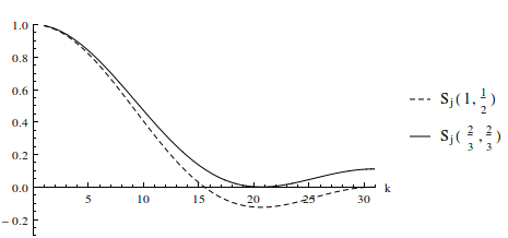
Figure 1: Eigenvalues of weighted-Jacobi with two steps $S_{j}^{2}$ for different $\omega$’s for $n=33$. We assume that the eigenvalues were continuous in $k$.

4 The error equation

Since we have explicit expressions for the eigenvalues of the two-grid iteration matrix $R^{TG}$ in (19) and of the corresponding eigenvectors in (16), which are linear combination of the eigenvectors of $A$, we can see which modes are damped more rapidly. To this end, we write the error $\mathbf{e}$ in terms of the eigenvectors of $R^{TG}$.

$$\mathbf{e}=\sum_{k=1}^{n-2}d_{i}\mathbf{b}_{k}=\sum_{k=1}^{(n-1)/2}d_{k}(\mathbf{v}_{k}+c_{1}(k)\mathbf{v}_{n-1-k})+\sum_{k=(n+1)/2}^{n-2}d_{k}(\mathbf{v}_{k}+c_{2}(k)\mathbf{v}_{n-1-k})$$

where $d_{k}$ is any constant, $c_{1}=c_{1}(k)$ and $c_{2}=c_{2}(k)$ which are given in (12) and (13), respectively. Since $\lambda_{k}(R^{TG})=0$ for $k=(n+1)/2...n-2$, after $m$ iterations, the error becomes

$$\mathbf{e}^{m}=\sum_{k=1}^{(n-1)/2}d_{k}\lambda_{k}^{m}(R^{TG})(\mathbf{v}_{k}+c_{1}(k)\mathbf{v}_{n-1-k})=\sum_{k=1}^{(n-1)/2}d_{k}\lambda_{k}^{m}(R^{TG})\mathbf{v}_{k}+\sum_{k=(n-1)/2}^{n-2}l_{k}\lambda_{n-1-k}^{m}(R^{TG})c_{1}(n-1-k)\mathbf{v}_{k}$$

where $\mathbf{e}^{m}$ stands for the error after $m$ iterations and $l_{k}$ is any constant. In above equation on the right, the first sum contains the smooth modes and the second sum contains oscillatory modes. The first eigenvalue $\lambda_{1}(\mathbf{R}^{TG})$ is associated with the smoothest and the most oscillatory mode. The eigenvalue $\lambda_{(n-1)/2}(R^{TG})$ is associated only with the eigenvector $\mathbf{v}_{(n-1)/2}$.

5 Conclusion

In this work, we provided an alternative Fourier analysis for multigrid applied to the Poisson problem in 1D. We related multigrid with the exact solver.

Note: This work is not going to be submitted to any journal. It is free to download and disseminate it.

References

[1]
W Briggs, V Henson, and S McCormick.
A Multigrid Tutorial, Second Edition.
Society for Industrial and Applied Mathematics, second edition, 2000.
[2]
Wolfgang Hackbusch.
Multi-Grid Methods and Applications.
Springer-Verlag Berlin Heidelberg, 1 edition, 1985.