Copula-based conformal prediction for Multi-Target Regression
Abstract
There are relatively few works dealing with conformal prediction for multi-task learning issues, and this is particularly true for multi-target regression. This paper focuses on the problem of providing valid (i.e., frequency calibrated) multi-variate predictions. To do so, we propose to use copula functions applied to deep neural networks for inductive conformal prediction. We show that the proposed method ensures efficiency and validity for multi-target regression problems on various data sets.
Keywords Inductive conformal prediction Copula functions Multi-target regression Deep neural networks.
1 Introduction
The most common supervised task in machine learning is to learn a single-task, single-output prediction model. However, such a setting can be ill-adapted to some problems and applications.
On the one hand, producing a single output can be undesirable when data is scarce and when producing reliable, possibly set-valued predictions is important (for instance in the medical domain where examples are very hard to collect for specific targets, and where predictions are used for critical decisions). Such an issue can be solved by using conformal prediction approaches [1]. It was initially proposed as a transductive online learning approach to provide set predictions (in the classification case) or interval predictions (in the case of regression) with a statistical guarantee depending on the probability of error tolerated by the user, but was then extended to handle inductive processes [2]. On the other hand, there are many situations where there are multiple, possibly correlated output variables to predict at once, and it is then natural to try to leverage such correlations to improve predictions. Such learning tasks are commonly called Multi-task in the literature [3].
Most research work on conformal prediction for multi-task learning focuses on the problem of multi-label prediction [4, 5], where each task is a binary classification one. Conformal prediction for multi-target regression has been less explored, with only a few studies dealing with it: Kuleshov et al. [6] provide a theoretical framework to use conformal predictors within manifold (e.g., to provide a mono-dimensional embedding of the multi-variate output), while Neeven and Smirnov [7] use a straightforward multi-target extension of a conformal single-output -nearest neighbor regressor [8] to provide weather forecasts. However, this latter essentially verifies validity (i.e., having well-calibrated outputs) for each individual target. Recently, we proposed a simple method to have an approximate validity for the multi-variate prediction [9], that generally provided overly conservative results.
In this paper, we propose a new conformal prediction method fitted to multi-target regression, that makes use of copulas [10] (a common tool to model dependence between multi-variate random variables) to provide valid multi-variate predictions. The interest of such a framework is that it remains very easy to apply while linking multi-variate conformal predictions to the theoretically sound framework that are copulas. Experiments also show that it works quite well, and allows to improve upon previous heuristics [9].
Section 2 provides a general overview of our problem: a brief introduction to conformal prediction and multi-target regression will be presented in Sections 2.1 and 2.2, before raising the problematic of applying conformal prediction to the multi-target regression setting in Section 2.3. We will then present our setting in Section 3: we will first recall the needed basic principles and theorems of copulas in Section 3.1, before detailing our conformal multi-target approach in Section 3.2. The experiments and their results are described in Section 4.
2 Inductive conformal prediction (ICP) for Multi-Target Regression
This section recalls the basics of inductive conformal regression and multi-target regression, before introducing the issues we will tackle in this paper.
2.1 Inductive conformal regression
In regression tasks, conformal prediction is a method that provides a statistical guarantee to the predictions by giving an interval prediction instead of a point prediction in the regression case. By statistical guarantee, it is meant that the set-valued predictions cover the true value with a given frequency, i.e., they are calibrated. It was first introduced as a transductive online learning approach [11] and then adapted to the inductive framework [2] where one uses a model induced from training examples to get conformal predictions for the new instances. The two desirable features in conformal regressors are (a) validity, i.e. the error rate does not exceed for each chosen confidence level , and (b) efficiency, meaning prediction intervals are as small as possible.
Let be the successive pairs of an object and its real-valued label , which constitute the observed examples. Assuming that the underlying random variables are exchangeable (a weaker condition than i.i.d.), we can predict for any new object by following the inductive conformal framework.
The first step consists of splitting the original data set into a training set and a calibration set , with . Then, an underlying algorithm is trained on to obtain the non-conformity measure , a measure that evaluates the strangeness of an example compared to other examples of a bag, called the non-conformity score. Hence, we can calculate the non-conformity score for an example compared to the other examples in the bag with .
By computing the non-conformity score for each example of using this equation, we get the sequence . When making a prediction for a new example , we use the underlying algorithm to associate to any possible prediction its non-conformity score , and calculate its p-value which indicates the proportion of less conforming examples than , with:
| (1) |
The final step before producing the conformal prediction consists of choosing the significance level to get a prediction set with a confidence level of , which is the statistical guarantee of coverage of the true value by the interval prediction such that
The most basic non-conformity measure in a regression setting is the absolute difference between the actual value and the predicted value by the underlying algorithm. The non-conformity score is then calculated as follows:
| (2) |
The sequence of non-conformity scores for all examples in are obtained and sorted in descending order. Then, we compute the index of the -percentile non-conformity score , based on the chosen significance level , such as:
| (3) |
Finally, the prediction interval for each new example , which covers the true output with probability is calculated as:
| (4) |
The drawback of this standard non-conformity measure is that all prediction intervals are equally sized () for a given confidence level. Adopting a normalized non-conformity measure instead provides personalized individual bounds for each new example by scaling the standard non-conformity measure with , a term that estimates the difficulty of predicting . This means that using a normalized non-conformity measure gives a smaller prediction interval for “easy” examples, and a bigger one for “hard” examples. Thus, two distinct examples with the same calculated by (2) will have two different interval predictions depending on their difficulty. In this case, the normalized non-conformity score is as follows:
| (5) |
Thus, we have:
| (6) |
which becomes an equality if the method is perfectly calibrated. For a new example , the prediction interval becomes :
| (7) |
The value can be defined in various ways. A popular approach proposed by Papadopoulos and Haralambous [12] consists of training a small neural network to estimate the error of the underlying algorithm by predicting the value . In this case, the non-conformity score is defined as:
| (8) |
where is a sensitivity parameter. With the significance level , we have:
| (9) |
For a new example , the prediction interval is:
| (10) |
Other approaches use different algorithms to normalize the non-conformity scores, such as regression trees [13] and -nearest neighbors [8]. Before introducing the problem of multi-target regression, let us first note that, assuming that our method is well-calibrated and that is associated to a random variable , (6) can be rewritten as
| (11) |
which will be instrumental when dealing with copulas and multi-variate outputs later on. Also note that this means that specifying a confidence uniquely defines a value .
2.2 Multi-target regression (MTR)
In multi-target regression, the feature space is the same as in standard regression, but the target space is made of real-valued targets. This means that observations are i.i.d pairs drawn from a probability distribution on , where each instance is associated to an dimensional real-valued target . The usual objective of multi-target regression is then to learn a predictor , i.e. to predict multiple outputs based on the input features characterizing the data set, which generalizes standard regression. There are two distinct approaches to treat MTR called algorithm adaptation and problem transformation methods.
For algorithm adaptation approaches, standard single-output regression algorithms are extended to the multi-target regression problem. Many models were adapted to the MTR problem, such as Support Vector Regressors [14], regression trees [15], kernel methods [16] and rule ensembles [17].
In problem transformation, one usually decomposes the initial multi-variate problems into several simpler problems, thus allowing the use of standard classification methods without the need for an adaptation that can be tricky or computationally costly. A prototypical example of such a transformation is the chaining method [18], where one predicts each target sequentially, using the output and predictions of previous targets as inputs for the next one, thus capturing some correlations between the targets.
As our goal here is not to produce a new MTR method, but rather to propose a flexible means to make their predictions reliable through conformal prediction, we will not make a more detailed review of those methods. The reader interested in different methods can consult for instance [18]. We will now detail how conformal prediction and MTR can be combined. Let us just mention that exploiting the possible relationships allow in general to improve performances of the methods [19, 20].
2.3 Inductive conformal prediction for Multi-Target Regression
As said before, previous studies about conformal MTR focused on providing valid and efficient inferences target-wise [7], thus potentially neglecting the potential advantages of exploiting target relations. Our main goal in this paper is to provide an easy conformal MTR method allowing to do so.
Within the MTR setting, we have a multi-dimensional output (we will use superscripts to denote the dimensions, and subscripts to denote sample indices) with the different individual real-valued targets. Let be respectively the lower and upper bounds of the interval predictions given by the non-conformity measure for each target given a new instance . We define the hyper-rectangle as the following Cartesian product:
| (12) |
This hyper-rectangle forms the volume to which a global prediction of a new example should belong in order to be valid, i.e. each single prediction for each individual target should be between the bounds of its interval prediction. With this view, the objective of the conformal prediction framework for MTR in the normalized setting is to satisfy a global significance level required by the user such that:
| (13) |
This probability can also be written as follows:
| (14) |
Thus, we need to find the individual non-conformity scores , defined for instance by target-wise confidence levels , such that we ensure a global confidence level . Extending (11) and considering the random variables , , we get:
| (15) |
Should we know the joint distribution in (15), and therefore the dependence relations between target predictions, it would be relatively easy to get the individual significance levels111Note that there may be multiple choices for such individual levels. Here we will fix them to be equal for simplicity. associated to the individual non-conformity scores such that we satisfy the chosen confidence level . Yet, such a joint distribution is usually unknown. The next section proposes a simple and efficient method to do so, leveraging the connection between (15) and copulas. Before doing that, note again that under the assumption that we are well calibrated, we can transform (15) into
| (16) |
where denotes here the joint cumulative distribution induced by .
3 Copula-based conformal Multi-Target Regression
This section introduces our approach to obtain valid or better conformal prediction in the multi-variate regression setting. We first recall some basics of copulas and refer to Nelsen [10] for a full introduction, before detailing how we apply them to conformal approaches.
3.1 Overview on copulas
A copula is a mathematical function that can describe the dependence between multiple random variables. The term “copula” was first introduced by Sklar [21] in his famous theorem, which is one of the fundamentals of copula theory, now known as Sklar’s theorem. However, these tools have already been used before, as for instance in Fréchet’s paper [22] and Höffding’s work [23, 24] (reprinted as [25]). Copulas are popular in the statistical and financial fields [26], but they are nowadays more and more used in other domains as well, such as hydrology [27], medicine [28], and machine learning [29].
Let be an -dimensional random vector composed of the random variables . Let its cumulative distribution function (c.d.f.) be . This c.d.f. carries two important pieces of information:
-
•
The c.d.f. of each random variable s.t. , for all
-
•
The dependence structure between them.
The objective of copulas is to isolate the dependence structure from the marginals by transforming them into uniformly distributed random variables and then expressing the dependence structure between the ’s. In other words, an -dimensional copula is a c.d.f. with standard uniform marginals. It is characterized by the following properties:
-
1.
is grounded, i.e. if for at least one , then .
-
2.
If all components of are equal to 1 except for all and , then .
-
3.
is -increasing, i.e., for all with :
The last inequality simply ensures that the copula is a well-defined c.d.f. inducing non-negative probability for every event. The idea of copulas is based on probability and quantile transformations [30]. Using these latter, we can see that all multivariate distribution functions include copulas and that we can use a mixture of univariate marginal distributions and a suitable copula to produce a multivariate distribution function. This is described in Sklar’s theorem [21] as follows:
Theorem 3.1 (Sklar’s theorem)
For any -dimensional cumulative distribution function (c.d.f.) with marginal distributions , there exists a copula such that:
| (17) |
If is continuous for all , then is unique.
Denoting the pseudo inverse of as [30], we can get from (17) that
| (18) |
There are a few noticeable copulas, among which are:
-
•
the product copula: ;
-
•
the Fréchet-Höffding upper bound copula 222 is a copula for all .: ;
-
•
the Fréchet-Höffding lower bound copula 333 is a copula if and only if .: .
While the product copula corresponds to classical stochastic independence, the Fréchet-Höffding bound copulas play an important role as they correspond to extreme cases of dependence [31]. Indeed, any -dimensional copula is such that
Another important class of copulas are so-called Archimedean copulas, which are based on generator functions of specific kinds. More precisely, a continuous, strictly decreasing, convex function satisfying is known as an Archimedean copula generator. It is known as a strict generator if . The generated copula is then given by
| (19) |
3.2 Copula-based conformal Multi-Target Regression
Let us now revisit our previous problem of finding the significance levels for each target so that the hyper-rectangle prediction covers the true value with confidence . Let us first consider (16). Following Sklar’s theorem, we have
where the second line is obtained from (6). Clearly, if we knew the copula , then we could search for values providing the desired global confidence.
A major issue is then to obtain or estimate the copula modelling the dependence structure between the targets and their confidence levels. As copulas are classically estimated from multi-variate observations, a simple means that we will use here is to estimate them from the non-conformity scores generated from the calibration set . Namely, if is the non-conformity score corresponding to the target of the example of for , we simply propose to estimate a copula from the matrix
| (20) |
3.3 On three specific copulas
We will now provide some detail about the copulas we performed experiments on. They have been chosen to go from the one requiring the most assumptions to the one requiring the least assumptions.
3.3.1 The Independent copula
The Independent copula means that the targets are considered as being independent, with no relationship between them. It is a strong assumption, but it does not require any estimation of the copula. In this case, (15) becomes:
If we assume that all equal the same value , then:
Thus, we simply obtain
| (21) |
This individual significance level is then used to calculate the different non-conformity scores for each target in the multi-target regression problem for the Independent copula.
3.3.2 The Gumbel copula
The Gumbel copula is a member of the Archimedean copula family which depends on only one parameter, and in this sense is a good representative of parametric copulas. It comes down to applying the generator function and its inverse to (19), resulting in the expression
| (22) |
In this case, we need to estimate the parameter . Since the marginals are unknown, we also need to estimate them. In our case, we will simply use the empirical c.d.f. induced by the non-conformity scores of matrix . An alternative would be to also assume a parametric form of the , but this seems in contradiction with the very spirit of non-conformity scores. In particular, we will denote by the empirical cumulative distribution such that
The parameter can then be estimated from matrix using the Maximum Pseudo-Likelihood Estimator [35] with a numerical optimization, for instance by using the Python library “copulae”444https://pypi.org/project/copulae/. Once this is obtained, we then get for a particular choice of that
| (23) | ||||
| (24) |
And we can search for values that will make this equation equal to , using the estimations . The solution is especially easy to obtain analytically if we consider that , as we then have that
and one can then obtain the corresponding non-conformity scores by replacing by .
We chose this particular family of Archimedean copulas because its lower bound is the Independent copula (as seen in Table 1). We can easily verify this by taking . Thus, we can capture independence if it is verified, and otherwise search in the direction of positive dependence. One reason for such a choice is that previous experiments [9] indicate that the product copula gives overly conservative results.
3.3.3 The Empirical copula
Parametric copulas, as all parametric models, have the advantage of requiring less data to be well estimated, while having the possibly important disadvantage that they induce some bias in the estimation, that is likely to grow as the number of target increases. The Empirical copula presents a non-parametric way of estimating the marginals directly from the observations [36, 37]. It is defined as follows [35]:
| (25) |
where is the indicator function of event , and the inequalities for need to be understood component-wise. are the pseudo-observations that replace the unknown marginal distributions, which are defined as:
| (26) |
where distributions are defined as before. Simply put, the Empirical copula corresponds to consider as our joint probability the Empirical joint cumulative distribution. We then have that
| (27) |
Using that , we can then search for values of , that will make (27) equal to . Note that in this case, even assuming that will require an algorithmic search, which is however easy as is an increasing function, meaning that we can use a simple dichotomic search.
4 Evaluation
In this section, we describe the experimental setting (underlying algorithm, data sets and performance metrics) and the results of our study.
4.1 Experimental setting
We choose to work with a deep neural network as the underlying algorithm. We keep the same underlying algorithm for all non-conformity measures, since our focus is to compare between the three copula functions chosen to get the different non-conformity scores.
To compute the non-conformity scores over the calibration set, we use the normalized non-conformity score given by (8) as described in [12], and predict simultaneously for all targets by a single multivariate multi-layer perceptron. In this case, represents the estimation of the underlying algorithm’s error. As mentioned before, the approach can be adapted to any conformal regression approach.
Experiments are conducted on normalized data with a mean of 0 and a standard deviation of 1 to simplify the deep neural network optimization, with a 10-fold cross validation to avoid the impact of biased results, and with a calibration set equal to of the training examples for all data sets. We take the value for the sensitivity parameter and do not optimize it when calculating the normalizing coefficient . After getting the proper training data , calibration data and test data for each fold, we follow the steps described below:
-
1.
Train the underlying algorithm (a deep neural network) on the proper training data . Its architecture is composed of a first dense layer applied to the input with “selu” activation (scaled exponential linear units [38]), three hidden dense layers with dropouts and “selu” activation, and a final dense layer with outputs and a linear activation.
-
2.
Predict and for calibration and test data respectively using the underlying algorithm.
-
3.
Train the normalizing multi-layer perceptron on the proper training data , corresponding to the error estimation of the underlying algorithm. The normalizing MLP consists of three hidden dense layers with “selu” activation and dropouts and a final dense layer with outputs for predicting all targets simultaneously.
-
4.
Predict and for calibration and test data respectively using the normalizing MLP.
-
5.
If needed, get an estimation555In the case of the Gumbel copula, we use a Maximum Pseudo-Likelihood Estimator with a numerical optimization using the BFGS algorithm of the copula from the matrix of calibration non-conformity scores.
-
6.
For each global significance level :
-
•
Get the individual significance level for and calculate for all targets using calibration data, according to the methods mentioned in Section 3.3.
-
•
Get the interval predictions for the test data with:
(28)
-
•
Remark 4.1
We choose for as we have no indication that individual targets should be treated with different degree of cautiousness. However, since copulas are functions from to , there is in principle no problem in considering different confidence degrees for different tasks, if an application calls for it. How to determine and elicit such degrees is however, to our knowledge, an open question.
The implementation was done using Python and Tensorflow. The copula part of our experiments was based on the book [35] and the Python library “copulae”.
| Names | Examples | Features | Targets |
|---|---|---|---|
| music origin [39] | 1059 | 68 | 2 |
| indoor loc [40] | 21049 | 520 | 3 |
| scpf [41] | 1137 | 23 | 3 |
| sgemm [42] | 241600 | 14 | 4 |
| rf1 [41] | 9125 | 64 | 8 |
| rf2 [41] | 9125 | 576 | 8 |
| scm1d [41] | 9803 | 280 | 16 |
| scm20d [41] | 8966 | 61 | 16 |
We use eight data sets with different numbers of targets and varying sizes. They are summarized in Table 2.
4.2 Results
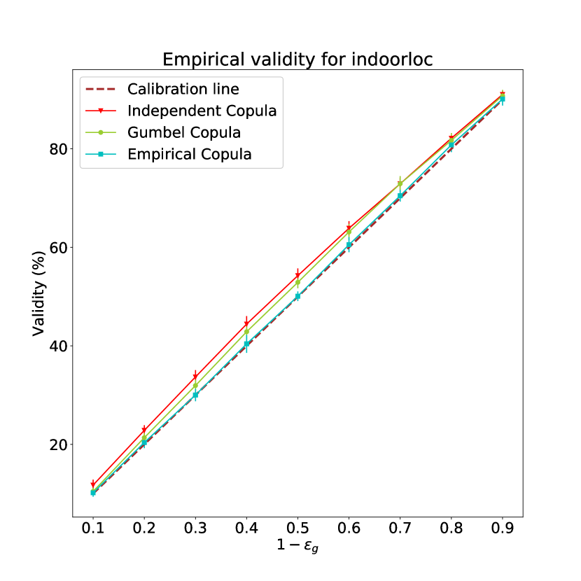
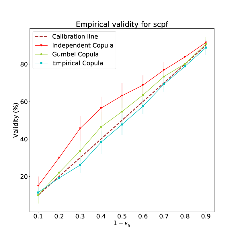
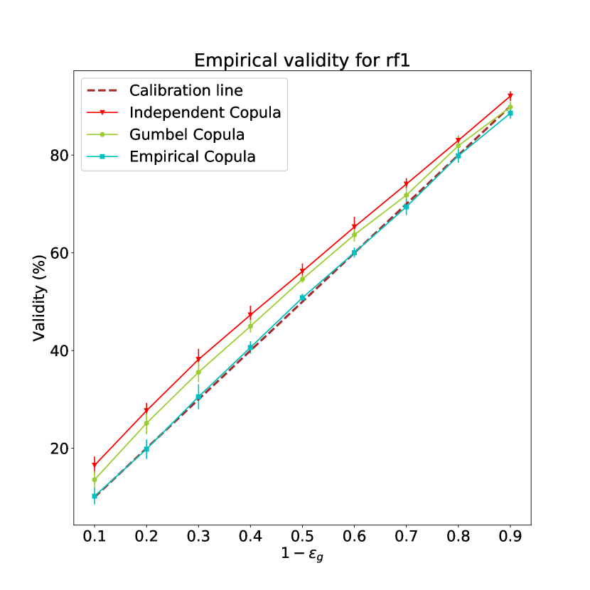
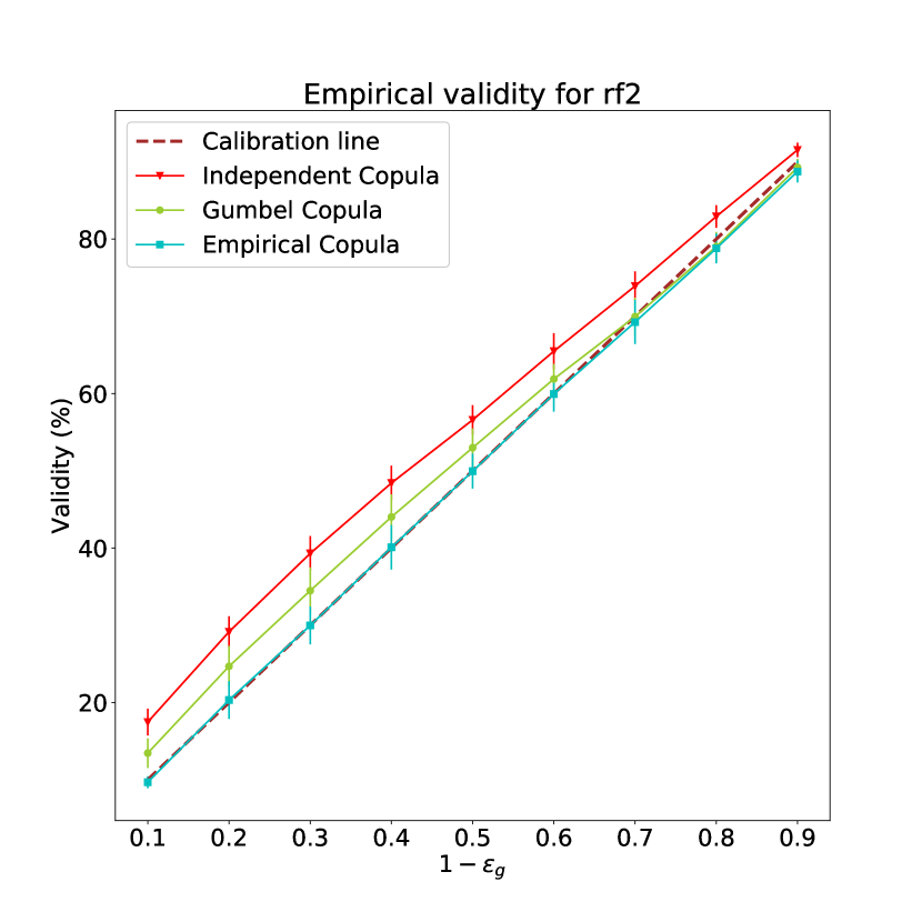
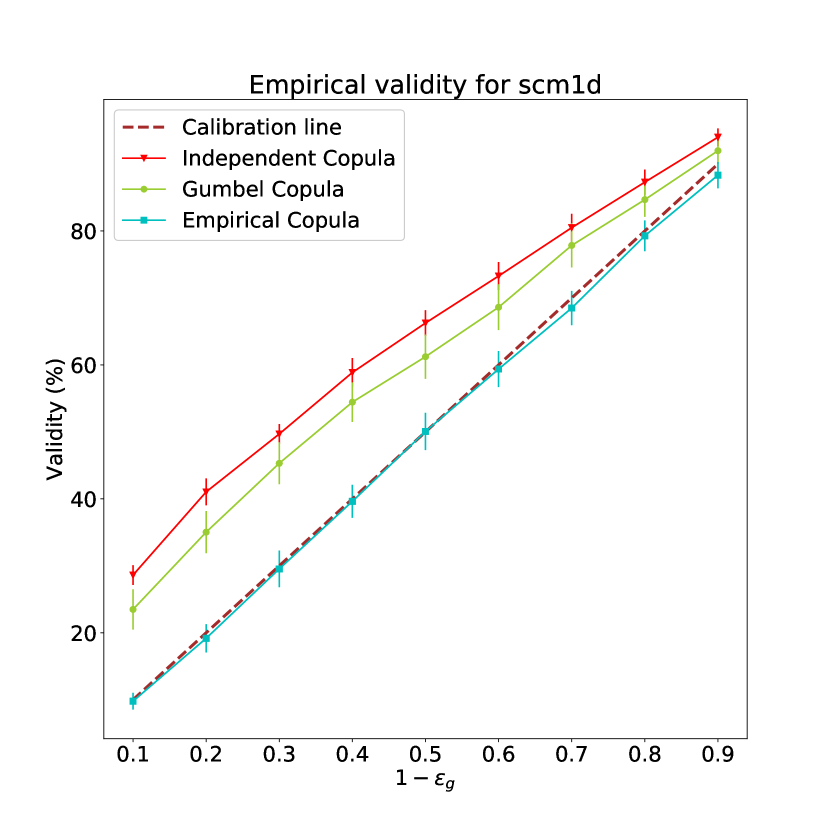
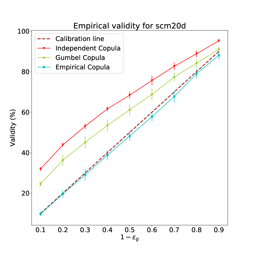
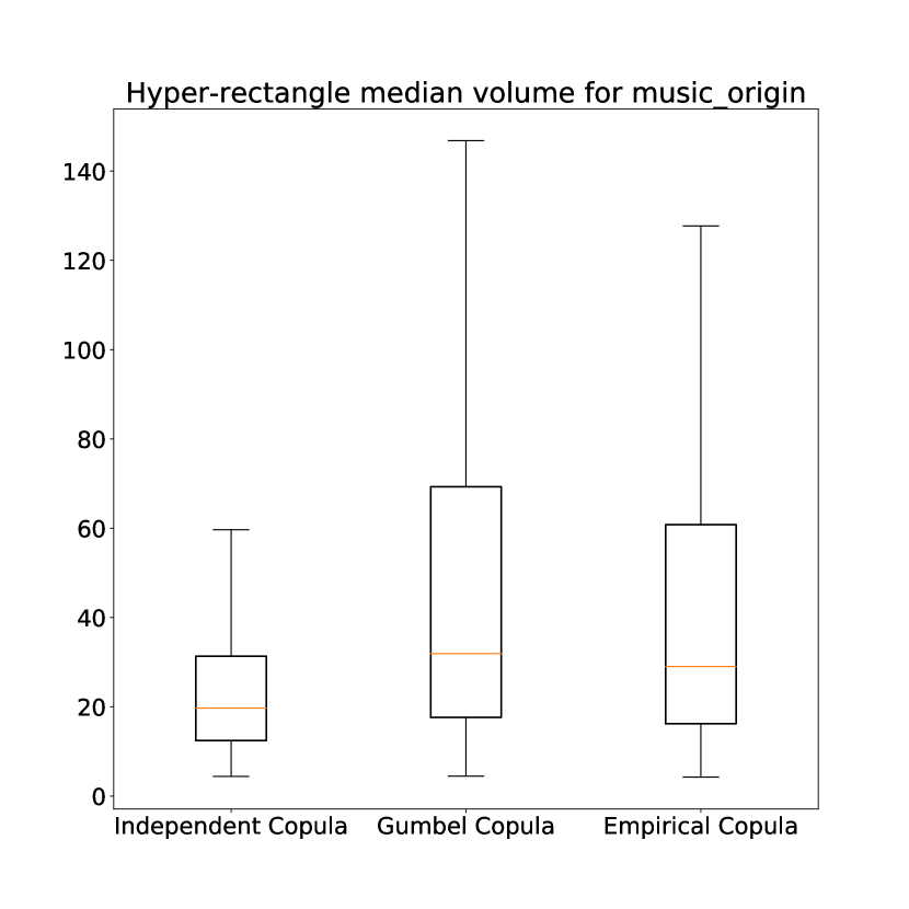
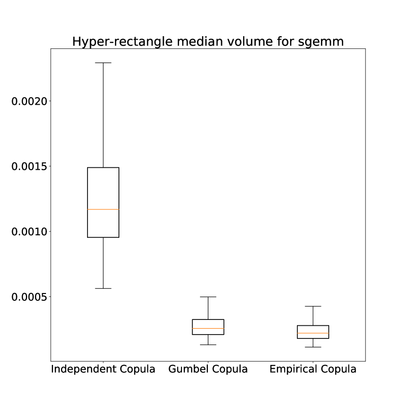
This section presents the results of our experiments, investigating in particular the validity and efficiency of the proposed approaches. Figures 1 and 2 detail these results for “music origin” and “sgemm”. The figures for all other data sets can be found in A.
To verify the validity of each non-conformity measure, we calculate the accuracy of each one and compare it with the calibration line. This line represents the case where the error rate is exactly equal to for a confidence level , which is the desired outcome of using conformal prediction. In multi-target regression, the accuracy is computed based on whether the observation belongs to the hyper-rectangle or not depending on the significance level . Thus, a correctly predicted example must verify that all its individual predictions for each individual target is in its corresponding individual interval predictions. Concretely, for each considered confidence level and test example , we obtain a prediction . From this, we can compute the empirical validity as the percentage of times that contains the true observed value, i.e.,
Doing it for several values of , we obtain a calibration curve that should be as close as possible to the identity function.
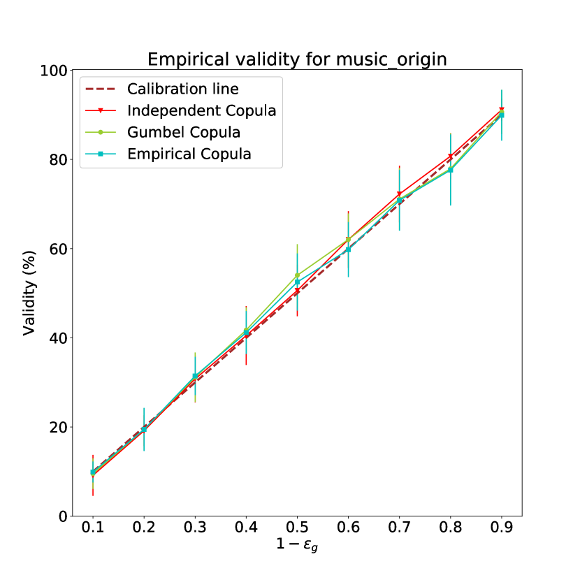
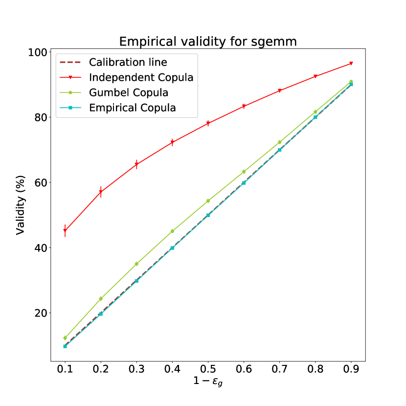
The results of the error rate or accuracy curves are shown in sub-figure a of each figure for the Independent, Gumbel and Empirical multivariate non-conformity measures. The outcomes clearly show that the best performance is obtained by using the Empirical copula, where the model is well calibrated. For most of the studied data sets, the Empirical copula accuracy curve is almost perfectly aligned with the calibration line, and thus almost exactly valid. This is due to the fact that Empirical copula functions non-parametrically estimate the marginals based on the observations, which enables the model to better adapt to the dependence structure of each data set. This dependence structure is neglected when using an Independent copula-based non-conformity measure, as the targets are treated as if they were independent, and so the link between them is not exploited when computing . This also means that the difference between the Empirical and the Independent copula-based non-conformity measures is bigger when there is a strong dependence between the non-conformity scores, and is an indication of the strength of this dependence. For instance, we can deduce that the targets are strongly related for “sgemm” by the big gap between the Independent and Empirical accuracy curves (sub-figure 2(a)). For the Gumbel copula, the accuracy curve is generally closer to the calibration line than the one for the Independent copula. This supports the existence of a dependence structure between the targets, since the lower bound of the Gumbel copula is the Independent copula, which means that if the targets were in fact independent, the two curves would perfectly match. This can be seen in sub-figure 1(a) for “music origin”, where the accuracy curves almost overlap all the time, meaning that the targets are likely to be independent.
From the empirical validity results, we also noticed that the Empirical copula non-conformity measure can be slightly invalid sometimes (sub-figure 4(a) for “scpf”). We explain this by the fewer number of examples, in which case one could use a more regularized form than the Empirical copula. However, when a lot of examples are available (for instance, more than 20000 observations for “sgemm”), the validity curve of the Empirical copula non-conformity measure is perfectly aligned with the calibration line, meaning that this measure is exactly valid (sub-figure 2(a)).
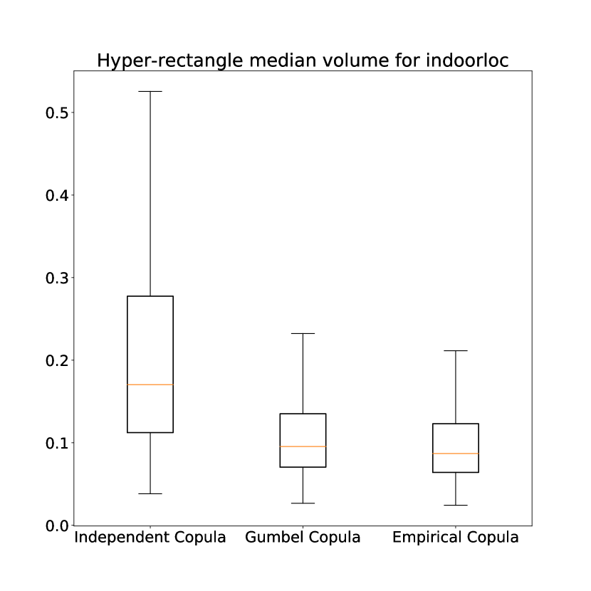
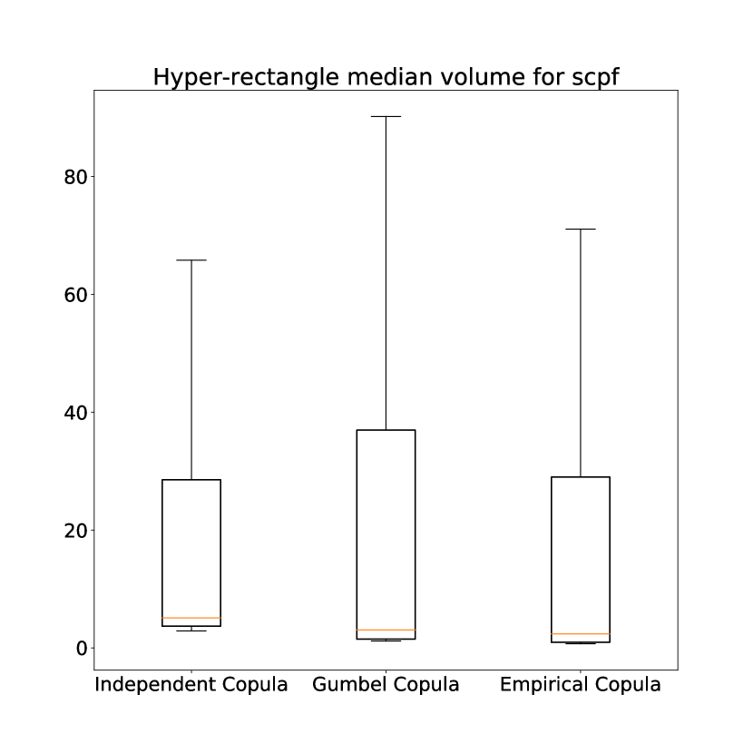
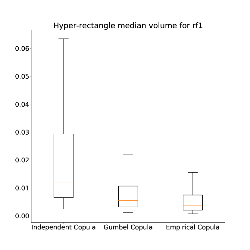
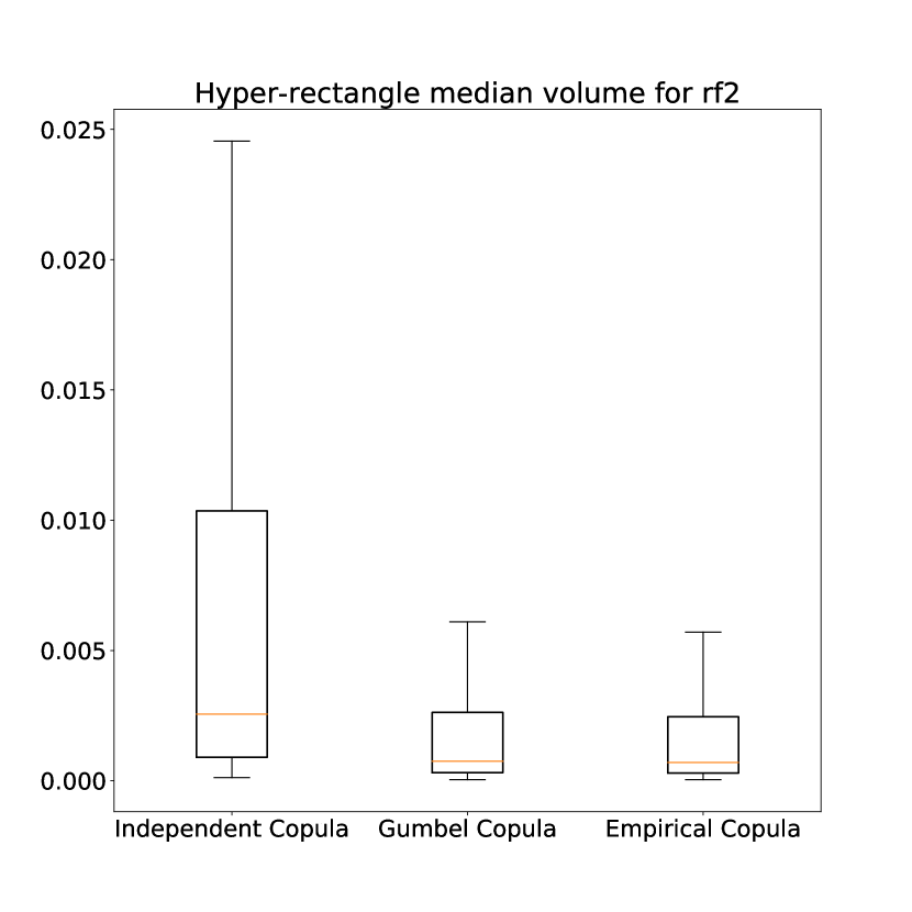
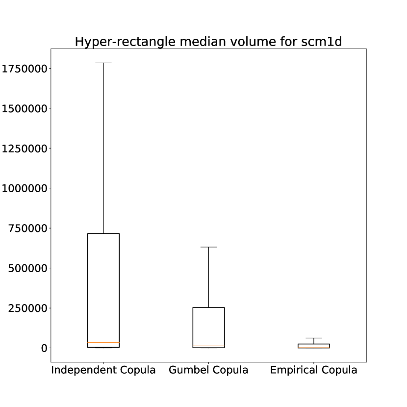
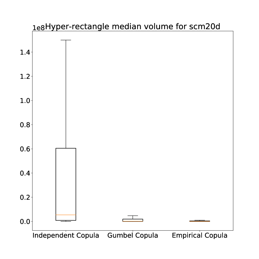
In single-output regression, efficiency is measured by the size of the intervals, and a method is all the more efficient as predicted intervals are small. To assess efficiency in multi-target regression, we can simply compute the volume of the obtained predictions , after (12). For each experiment, we then compute the median value of those hyper-rectangle volumes (for the estimation to be robust against very large hyper-rectangles).
Efficiency results are shown in sub-figure b for all data sets for . They show that, in general, the Independent copula has a bigger median hyper-rectangle volume compared to the Gumbel and Empirical copulas, especially in those cases where the existence of a dependence structure is confirmed by the calibration curves. This is due to the fact that using an Independent copula ignores the dependence between the non-conformity scores, which leads to an over-estimation of the global hyper-rectangle error. This impact is avoided when using the Empirical copula because it takes advantage of the dependence structure to construct better interval predictions. Another remark concerning efficiency is that the box plots for Empirical copula are tighter than the other two, which shows that the values are homogeneous on all folds compared to the Independent copula for instance, where the variation is much more visible.
The empirical validity and hyper-rectangle median volume results are summarized in Tables 3 and 4. The validity simply provides the average difference between a perfect calibration (the identity function) and the observed curve for each copula. This means, in particular, that a negative value indicates that the observed frequency is in average below the specified confidence degree.
Data sets Independent Gumbel Empirical music origin indoor loc scpf sgemm rf1 rf2 scm1d scm20d
Data sets Independent Gumbel Empirical music origin indoor loc scpf sgemm rf1 rf2 scm1d scm20d
The numbers confirm our previous observations on the graphs, as the average gap is systematically higher for the Independent copula and lower for the Empirical one, with Gumbel in-between. We can however notice that while the Empirical copula provides the best results, it is also often a bit under the calibration line, indicating that if conservativeness is to be sought, one should maybe prefer the Gumbel copula. About the same conclusions can be given regarding efficiency, with the Empirical copula giving the best results and the Independent one the worst.
5 Conclusion and discussion
In this paper, we provided a quite easy and flexible way to obtain valid conformal predictions in a multi-variate regression setting. We did so by exploiting a link between non-conformity scores and copulas, a commonly used tool to model multi-variate distribution.
Experiments on various data sets for a small choice of representative copulas show that the method indeed allows to improve upon the naive independence assumption. Those first results indicate in particular that while parametric, simple copulas may provide valid results for some data sets, more complex copulas may be needed in general to obtain well calibrated predictions, with the cost that good estimations of such copulas require a lot of calibration data.
As future lines of work, we would like to explore further the flexibility of our framework, for instance by exploring the possibility of using vines [43] to model complex dependencies, or by proposing protocols allowing to obtain from different individual, user-defined confidence degrees, taking up on our Remark 4.1.
Finally, while we mostly focused on multi-variate regression in the present paper, it would be interesting to try to extend the current approach to other multi-task settings, such as multi-label problems. A possibility could be to make such problems continuous, as proposed for instance by Liu [29].
6 Acknowledgments
This research was supported by the UTC foundation.
References
- [1] Glenn Shafer and Vladimir Vovk. A tutorial on conformal prediction. Journal of Machine Learning Research, 9(Mar):371–421, 2008.
- [2] Harris Papadopoulos, Kostas Proedrou, Volodya Vovk, and Alex Gammerman. Inductive confidence machines for regression. In European Conference on Machine Learning, pages 345–356. Springer, 2002.
- [3] Rich Caruana. A dozen tricks with multitask learning. In Neural networks: tricks of the trade, pages 165–191. Springer, 1998.
- [4] Huazhen Wang, Xin Liu, Ilia Nouretdinov, and Zhiyuan Luo. A comparison of three implementations of multi-label conformal prediction. In International Symposium on Statistical Learning and Data Sciences, pages 241–250. Springer, 2015.
- [5] Ran Wang, Sam Kwong, Xu Wang, and Yuheng Jia. Active k-labelsets ensemble for multi-label classification. Pattern Recognition, page 107583, 2020.
- [6] Alexander Kuleshov, Alexander Bernstein, and Evgeny Burnaev. Conformal prediction in manifold learning. In Conformal and Probabilistic Prediction and Applications, pages 234–253, 2018.
- [7] Jelmer Neeven and Evgueni Smirnov. Conformal stacked weather forecasting. In Conformal and Probabilistic Prediction and Applications, pages 220–233, 2018.
- [8] Harris Papadopoulos, Vladimir Vovk, and Alexander Gammerman. Regression conformal prediction with nearest neighbours. Journal of Artificial Intelligence Research, 40:815–840, 2011.
- [9] Soundouss Messoudi, Sébastien Destercke, and Sylvain Rousseau. Conformal multi-target regression using neural networks. In Conformal and Probabilistic Prediction and Applications, pages 65–83. PMLR, 2020.
- [10] Roger B Nelsen. An introduction to copulas, volume 139 of. Lecture Notes in Statistics, 1999.
- [11] Alex Gammerman, Volodya Vovk, and Vladimir Vapnik. Learning by transduction. Proceedings of the Fourteenth Conference on Uncertainty in Artificial Intelligence, page 148–155, 1998.
- [12] Harris Papadopoulos and Haris Haralambous. Reliable prediction intervals with regression neural networks. Neural Networks, 24(8):842–851, 2011.
- [13] Ulf Johansson, Henrik Linusson, Tuve Löfström, and Henrik Boström. Interpretable regression trees using conformal prediction. Expert systems with applications, 97:394–404, 2018.
- [14] Matilde Sánchez-Fernández, Mario de Prado-Cumplido, Jerónimo Arenas-García, and Fernando Pérez-Cruz. Svm multiregression for nonlinear channel estimation in multiple-input multiple-output systems. IEEE transactions on signal processing, 52(8):2298–2307, 2004.
- [15] Glenn De’Ath. Multivariate regression trees: a new technique for modeling species–environment relationships. Ecology, 83(4):1105–1117, 2002.
- [16] Luca Baldassarre, Lorenzo Rosasco, Annalisa Barla, and Alessandro Verri. Multi-output learning via spectral filtering. Machine learning, 87(3):259–301, 2012.
- [17] Timo Aho, Bernard Ženko, and Sašo Džeroski. Rule ensembles for multi-target regression. In 2009 Ninth IEEE International Conference on Data Mining, pages 21–30. IEEE, 2009.
- [18] Eleftherios Spyromitros-Xioufis, Grigorios Tsoumakas, William Groves, and Ioannis Vlahavas. Multi-target regression via input space expansion: treating targets as inputs. Machine Learning, 104(1):55–98, 2016.
- [19] Sebastian Ruder. An overview of multi-task learning in deep neural networks. arXiv preprint arXiv:1706.05098, 2017.
- [20] Rich Caruana. Multitask learning: A knowledge-based source of inductive bias icml. Google Scholar Google Scholar Digital Library Digital Library, 1993.
- [21] M Sklar. Fonctions de repartition an dimensions et leurs marges. Publ. inst. statist. univ. Paris, 8:229–231, 1959.
- [22] Maurice Fréchet. Sur les tableaux de corrélation dont les marges sont données. Ann. Univ. Lyon, 3^ e serie, Sciences, Sect. A, 14:53–77, 1951.
- [23] Wassilij Höffding. Masstabinvariante korrelationstheorie. Schriften des Mathematischen Instituts und Instituts fur Angewandte Mathematik der Universitat Berlin, 5:181–233, 1940.
- [24] Wassily Höffding. Masstabinvariante korrelationsmasse für diskontinuierliche verteilungen. Archiv für mathematische Wirtschafts-und Sozialforschung, 7:49–70, 1941.
- [25] Wassily Höffding. Scale—invariant correlation theory. In The collected works of Wassily Höffding, pages 57–107. Springer, 1994.
- [26] Paul Embrechts, Alexander McNeil, and Daniel Straumann. Correlation and dependence in risk management: properties and pitfalls. Risk management: value at risk and beyond, 1:176–223, 2002.
- [27] Anne-Catherine Favre, Salaheddine El Adlouni, Luc Perreault, Nathalie Thiémonge, and Bernard Bobée. Multivariate hydrological frequency analysis using copulas. Water resources research, 40(1), 2004.
- [28] Aristidis K Nikoloulopoulos and Dimitris Karlis. Multivariate logit copula model with an application to dental data. Statistics in Medicine, 27(30):6393–6406, 2008.
- [29] Weiwei Liu. Copula multi-label learning. In Advances in Neural Information Processing Systems, pages 6337–6346, 2019.
- [30] Alexander J McNeil, Rüdiger Frey, and Paul Embrechts. Quantitative risk management: concepts, techniques and tools-revised edition. Princeton university press, 2015.
- [31] Thorsten Schmidt. Coping with copulas. Copulas-From theory to application in finance, pages 3–34, 2007.
- [32] Emil Julius Gumbel. Distributions des valeurs extremes en plusiers dimensions. Publ. Inst. Statist. Univ. Paris, 9:171–173, 1960.
- [33] Christian Genest and Louis-Paul Rivest. Statistical inference procedures for bivariate archimedean copulas. Journal of the American statistical Association, 88(423):1034–1043, 1993.
- [34] Maurice J Frank. On the simultaneous associativity off (x, y) andx+y- f (x, y). Aequationes mathematicae, 19(1):194–226, 1979.
- [35] Marius Hofert, Ivan Kojadinovic, Martin Mächler, and Jun Yan. Elements of copula modeling with R. Springer, 2019.
- [36] Ludger Ruschendorf. Asymptotic distributions of multivariate rank order statistics. The Annals of Statistics, pages 912–923, 1976.
- [37] Frederik Hendrik Ruymgaart. Asymptotic theory of rank tests for independence. MC Tracts, 1978.
- [38] Günter Klambauer, Thomas Unterthiner, Andreas Mayr, and Sepp Hochreiter. Self-normalizing neural networks. In Advances in neural information processing systems, pages 971–980, 2017.
- [39] Fang Zhou, Q Claire, and Ross D King. Predicting the geographical origin of music. In 2014 IEEE International Conference on Data Mining, pages 1115–1120. IEEE, 2014.
- [40] Joaquín Torres-Sospedra, Raúl Montoliu, Adolfo Martínez-Usó, Joan P Avariento, Tomás J Arnau, Mauri Benedito-Bordonau, and Joaquín Huerta. Ujiindoorloc: A new multi-building and multi-floor database for wlan fingerprint-based indoor localization problems. In 2014 international conference on indoor positioning and indoor navigation (IPIN), pages 261–270. IEEE, 2014.
- [41] Grigorios Tsoumakas, Eleftherios Spyromitros-Xioufis, Jozef Vilcek, and Ioannis Vlahavas. Mulan: A java library for multi-label learning. Journal of Machine Learning Research, 12(71):2411–2414, 2011.
- [42] Cedric Nugteren and Valeriu Codreanu. Cltune: A generic auto-tuner for opencl kernels. In 2015 IEEE 9th International Symposium on Embedded Multicore/Many-core Systems-on-Chip, pages 195–202. IEEE, 2015.
- [43] Harry Joe and Dorota Kurowicka. Dependence modeling: vine copula handbook. World Scientific, 2011.
Appendix A Validity and efficiency figures
This appendix contains the figures for empirical validity and hyper-rectangle median volume for all remaining data sets.