Seroprevalence of SARS-CoV-2 antibodies in South Korea

Abstract

In $\displaystyle 2020$, Korea Disease Control and Prevention Agency reported three rounds of surveys on seroprevalence of severe acute respiratory syndrome coronavirus 2 (SARS-CoV-2) antibodies in South Korea. We analyze the seroprevalence surveys using a Bayesian method with an informative prior distribution on the seroprevalence parameter, and the sensitivity and specificity of the diagnostic test. We construct the informative prior using the posterior distribution obtained from the clinical evaluation data based on the plaque reduction neutralization test. The constraint of the seroprevalence parameter induced from the known confirmed cornonavirus 2019 cases can be imposed naturally in the proposed Bayesian model. We also prove that the confidence interval of the seroprevalence parameter based on the Rao’s test can be the empty set, while the Bayesian method renders a reasonable interval estimator. As of the $\displaystyle 30$th of October 2020, the $\displaystyle 95\%$ credible interval of the estimated SARS-CoV-2 positive population does not exceed $\displaystyle 307,448$, approximately $\displaystyle 0.6\%$ of the Korean population.

1 Introduction

In December 2019, the Chinese government reported a cluster of pneumonia patients of unknown cause in Wuhan, China. It was found that an unknown betacoronavirus causes the disease (Zhu et al., 2020). The Coronaviridae Study Group (CSG) of the International Committee on Taxonomy of Viruses has named the virus as severe acute respiratory syndrome coronavirus 2 (SARS-CoV-2), due to the similarity to SARS-CoV (Gorbalenya et al., 2020). The World Health Organization (WHO) also has named the disease caused by SARS-CoV-2 as COVID-19, short for coronavirus disease 2019 (The World Health Organization, 2020a). As of January 10, 2021, over $\displaystyle 90,000,000$ people in the world are confirmed positive for COVID-19, and there are over $\displaystyle 68,000$ confirmed cases in South Korea.

Most statistical approaches use the number of confirmed cases to assess the spread of infectious diseases in a population. However, the number of confirmed cases does not include those that are infected but not detected. A seroprevalence survey can be an alternative in this case. The seroprevalence is the number of people with antibodies to the virus in a population. The WHO (2020b) proposes to analyze seroprevalence surveys for the inference on the spread of a novel coronavirus. Seroprevalence surveys have been conducted in many countries, and the results are collected in Serotracker, a global seroprevalence dashboard (Arora et al., 2020). According to the recent update on December $\displaystyle 12$, $\displaystyle 2020$, Serotracker provides the survey results of $\displaystyle 56$ countries based on $\displaystyle 491$ studies.

The seroprevalence survey data can be analyzed under either the assumption that the diagnostic tests used in the survey are $\displaystyle 100\%$ accurate or the assumption that the tests are not $\displaystyle 100\%$ accurate. We will term these assumptions as the accuracy assumption and the inaccuracy assumption, respectively. Under the accuracy assumption, Song et al. (2020) and Noh et al. (2020) analyzed outpatient data sets in southwestern Seoul and Daegu, respectively, and estimated the seroprevalence. Although the statistical models are simpler under the accuracy assumption, the estimates can be biased unless the assumption is met as pointed out in Diggle (2011). Under the inaccuracy assumption, Diggle (2011) proposed a corrected prevalence estimator and Silveira et al. (2020) constructed a confidence interval of the seroprevalence using a resampling method. In an analysis of a seroprevalence survey data of southern Brazil, Silveira et al. (2020) showed that confidence intervals can be $\displaystyle\{0\}$, which is hardly reliable. See Supplementary Table 2 in Silveira et al. (2020). In Section 3, we also prove that the confidence interval constructed from the Rao’s test using the duality theorem (Bickel and Doksum, 2015) can be the empty set. These examples show that the frequentist confidence intervals of the seroprevalence under the inaccuracy assumption can be unreliable.

In this paper, we propose a Bayesian method under the inaccuracy assumption and apply the proposed method to the seroprevalence surveys of the South Korean population conducted in $\displaystyle 2020$ (Korea Disease Control and Prevention Agency, 2021). We use the posterior distribution obtained from the Bayesian model of the clinical evaluation data (Kohmer et al., 2020) as the informative prior distribution of the sensitivity and specificity on the diagnostic test.

The rest of the paper is organized as follows. In the next section, we describe the seroprevalence surveys of SARS-CoV-2 motivating this work and the plaque reduction neutralization test for detection of SARS-CoV-2 antibodies. In Section 3, we conduct a frequentist analysis and discuss the phenomenon of empty confidence sets. In Section 4, we propose a Bayesian method for the seroepidemiological survey that gives nonempty interval estimates, and analyze the seroprevalence surveys of the South Korean population using the proposed Bayesian method. We conclude the paper with a discussion section.

2 Seroepidemiological surveys and clinical evaluation of a serology test

2.1 Seroepidemiological surveys of SARS-CoV-2 in South Korea

Korea Disease Control and Prevention Agency (KDCA) conducted three rounds of seroprevalence surveys of SARS-CoV-2 for South Korean population in 2020. KDCA used the sets of samples collected in the Korea National Health and Nutrition Examination Survey (KNHNES), which is a regular national survey to investigate the health and nutritional status of South Koreans since 1998 (Kwon et al., 2014), as the samples of the seroprevalance surveys. KDCA performed a serology test for SARS-CoV-2 to the residual serums, and the test results (Korea Disease Control and Prevention Agency, 2021) are summarised in Table 1. In Table 1, the periods during which the samples are collected are also given.

Table 1: The result of the seroprevalence surveys in 2020 (Korea Disease Control and Prevention Agency, 2021). The column of the announcement date represents dates when KDCA reports the results of the surveys. The column of the collection period represents the periods during which the sets of samples are collected.

Accouncement date	Collection period	Number of samples	Number of test-positive samples
9th of July	4.21. $\displaystyle\sim$ 6.16.	$\displaystyle 1500$	$\displaystyle 0$
11th of September	6.10. $\displaystyle\sim$ 8.13.	$\displaystyle 1440$	$\displaystyle 1$
23th of November	8.14. $\displaystyle\sim$ 10.31.	$\displaystyle 1379$	$\displaystyle 3$

2.2 Clinical evaluation of plaque reduction neutralization test for SARS-CoV-2 antibodies

When KDCA performed a serology test for SARS-CoV-2, KDCA used their in-house plaque reduction neutralization test (PRNT). In the PRNT, serum samples are tested for their neutralization capacity against SARS-CoV-2. To estimate the sensitivity and specificity of PRNT methods for SARS-CoV-2 empirically, we use a set of clinical evaluation data (Table 2) which is conducted by Kohmer et al. (2020).

Table 2: The data of clinical evaluation of the PRNT by Kohmer et al. (2020). The columns represent the true states of samples. The true state of a sample refers to whether the sample has the antibodies against SARS-CoV-2 in reality.

		True state
		Positive	Negative	Total
Test results of the PRNT	Positive	$\displaystyle 42$	$\displaystyle 1$	$\displaystyle 43$
	Negative	$\displaystyle 3$	$\displaystyle 34$	$\displaystyle 37$
	Total	$\displaystyle 45$	$\displaystyle 35$	$\displaystyle 80$

3 Maximum likelihood estimator and a confidence interval

Under the inaccuracy assumption, we specify a statistical model for seroprevalance surveys, and present the maximum likelihood estimator and a confidence interval of the seroprevalance. We assume that the sensitivity and specificity of serology test are fixed values for the estimator and the confidence interval. Note that the sensitivity and specificity are the probabilities that the positive has the positive test result and the negative has the negative test result, respectively.

We define seroprevalance parameter, $\displaystyle\theta$, as the proportion of those who have antibodies against SARS-CoV-2 in the population. Let $\displaystyle N$ be the number of samples of seroprevalence survey, $\displaystyle X$ be the number of test-positive samples by serology test, and $\displaystyle p_{+}$ and $\displaystyle p_{-}$ denote the sensitivity and specificity of the serology test, respectively. We assume $\displaystyle X$ is generated from the binomial distribution:

$$\displaystyle X\sim Binom\left(N,\theta p_{+}+(1-\theta)(1-p_{-})\right),$$ (1)

where $\displaystyle Binom(n,p)$ denotes the binomial distribution with parameters $\displaystyle n\in\mathbb{N}$ and $\displaystyle p\in[0,1]$. When $\displaystyle p_{+}$ and $\displaystyle p_{-}$ are known, the maximum likelihood estimator for $\displaystyle\theta$ is as follows. If $\displaystyle 1-p_{-}<p_{+}$, then

$$\displaystyle\hat{\theta}^{MLE}=\begin{cases}0&\text{if }X\leq N(1-p_{-})\\ 1&\text{if }X\geq Np_{+}\\ \frac{X/N-(1-p_{-})}{p_{+}+p_{-}-1}&\text{if }N(1-p_{-})<X<Np_{+},\end{cases}$$ (2)

and if $\displaystyle p_{+}<1-p_{-}$, then

$$\displaystyle\hat{\theta}^{MLE}=\begin{cases}0&\text{if }X\geq N(1-p_{-})\\ 1&\text{if }X\leq Np_{+}\\ \frac{X/N-(1-p_{-})}{p_{+}+p_{-}-1}&\text{if }Np_{+}<X<N(1-p_{-}).\end{cases}$$

Note if the number of test-positive samples is small or large enough, the maximum likelihood estimator can be $\displaystyle 0$ or $\displaystyle 1$. This means that nobody or everybody in the population has antibodies against SARS-CoV-2, which is hardly reliable.

We construct a confidence interval of $\displaystyle\theta$ from Rao’s test (Rao, 1948) using the duality thoerem (Bickel and Doksum, 2015), and show that when $\displaystyle X$ is too small or large, the confidence interval can be the empty set. Let $\displaystyle A(\theta_{0})=[l_{\theta_{0}},u_{\theta_{0}}]$ be the $\displaystyle 100(1-\alpha)\%$ acceptance interval of the Rao’s test under the null hypothesis $\displaystyle H_{0}:\theta=\theta_{0}$. By the duality theorem $\displaystyle S(X)=\{\theta_{0}\in[0,1]:X\in A(\theta_{0})\}$ is a $\displaystyle 100(1-\alpha)\%$ confidence interval for $\displaystyle\theta$. Theorem 3.1 gives the acceptance interval, $\displaystyle A(\theta_{0})$, and the condition that the confidence interval $\displaystyle S(X)$ is the empty set.

Theorem 3.1

Consider the model (1).

1. The $\displaystyle 100(1-\alpha)\%$ acceptance region of the test

   $$H_{0}:\theta=\theta_{0}\text{ vs }H_{1}:\theta\neq\theta_{0}$$

   by the Rao’s Score test is given as

   $$\displaystyle[l_{\theta_{0}},u_{\theta_{0}}]=[N\theta^{*}_{0}-\{N\chi^{2}_{0.05}(1)\theta^{*}_{0}(1-\theta^{*}_{0})\}^{1/2},N\theta^{*}_{0}+\{N\chi^{2}_{0.05}(1)\theta^{*}_{0}(1-\theta^{*}_{0})\}^{1/2}],$$

   where $\displaystyle\theta^{*}_{0}=\theta_{0}p_{+}+(1-\theta_{0})(1-p_{-})$ and $\displaystyle\chi^{2}_{\alpha}(1)$ is $\displaystyle(1-\alpha)100\%$ quantile of chi-square distribution with $\displaystyle 1$ degree of freedom.

2. If

   $$\displaystyle X<\inf_{\theta_{0}\in[0,1]}l_{\theta_{0}}\text{ or }X>\sup_{\theta_{0}\in[0,1]}u_{\theta_{0}},$$ (3)

   the $\displaystyle 100(1-\alpha)\%$ confidence interval $\displaystyle S(X)=\{\theta_{0}\in[0,1]:X\in A(\theta_{0})\}$ is the empty set.

• (a) Let $\displaystyle\theta^{*}=\theta p_{+}+(1-\theta)(1-p_{-})$ and

  $$L(\theta)=L(\theta;N,X)=\binom{N}{X}\theta^{X}(1-\theta)^{N-X}.$$

  The score statistics is

  $$\displaystyle\Big{(}\frac{d\log L(\theta)}{d\theta}\Big{)}_{\theta=\theta_{0}}^{2}\Big{[}E\Big{(}-\frac{d^{2}\log L(\theta)}{d\theta^{2}}\Big{)}_{\theta=\theta_{0}}\Big{]}^{-1} \displaystyle= \displaystyle\Big{(}\frac{d\log L(\theta)}{d\theta^{*}}\Big{)}_{\theta=\theta_{0}}^{2}\Big{[}E\Big{(}-\frac{d^{2}\log L(\theta)}{d(\theta^{*})^{2}}\Big{)}_{\theta=\theta_{0}}\Big{]}^{-1}$$

  $$\displaystyle= \displaystyle\frac{(X-N\theta_{0}^{*})^{2}}{N\theta_{0}^{*}}+\frac{(N-X-N(1-\theta_{0}^{*}))^{2}}{N(1-\theta_{0}^{*})}$$

  $$\displaystyle= \displaystyle\frac{(X-N\theta_{0}^{*})^{2}}{N\theta_{0}^{*}(1-\theta_{0}^{*})}.$$

  Then, $\displaystyle 100(1-\alpha)\%$ acceptance interval is

  $$\displaystyle A(\theta_{0}) \displaystyle= \displaystyle\Big{\{}X:\frac{(X-N\theta_{0}^{*})^{2}}{N\theta_{0}^{*}(1-\theta_{0}^{*})}\leq\chi^{2}_{\alpha}(1)\Big{\}}$$

  $$\displaystyle= \displaystyle\{X:|X-N\theta_{0}^{*}|\leq\{\chi^{2}_{\alpha}(1)Np_{0}^{*}(1-\theta_{0}^{*})\}^{1/2}\},$$

  which proves (a).

  (b) If

  $$\displaystyle X<\inf_{\theta_{0}\in[0,1]}l_{\theta_{0}}\text{ or }X>\sup_{\theta_{0}\in[0,1]}u_{\theta_{0}},$$

  then $\displaystyle X\notin A(\theta_{0})$ for all $\displaystyle\theta_{0}\in[0,1]$. It implies the confidence interval of $\displaystyle X$ is the empty set. This completes the proof. $\displaystyle\blacksquare$

The intuitive reason for the empty confidence interval is as follows. The set of sampling distributions for $\displaystyle X$ is

$$\displaystyle\left\{Binom(N,\theta):(1-p_{-})\leq\theta\leq p_{+}\right\}.$$

When $\displaystyle X/N$ is smaller (larger) than $\displaystyle 1-p_{-}$ ($\displaystyle p_{+}$), the probability that $\displaystyle X$ is observed is small for every sampling distribution in the set. This makes test decisions rejected for every null hypothesis. Thus, the extreme $\displaystyle X$ implies $\displaystyle p_{-}$ and $\displaystyle p_{+}$ are doubtful.

For the three rounds of surveys given in Table 1, we show all the maximum likelihood estimators are zero and the confidence intervals are the empty set. We assume the fixed $\displaystyle(p_{+},p_{-})$ to be $\displaystyle(42/45,34/35)$, which is calculated from the clinical evaluation data (Table 2) and formula $\displaystyle(r_{++}/r_{\cdot+},r_{--}/r_{\cdot-})$ according to the notation in Table 3. Based on equation (2), all the maximum likelihood estimatiors are zero, since values of $\displaystyle N(1-p_{-})$ are $\displaystyle 42.9$, $\displaystyle 41.1$ and $\displaystyle 39.4$ which are all larger than the observed $\displaystyle X$s. The confidence intervals are the empty set since values of $\displaystyle\inf_{\theta\in[0,1]}l_{\theta}$ are $\displaystyle 30.2$, $\displaystyle 28.8$ and $\displaystyle 27.3$ which satisfy condition (3) in Theorem 3.1.

4 A Bayesian method with informative prior distributions

We propose a Bayesian method that avoids the empty confidence set problem. For the Bayesian analysis of model (1), we assign prior distributions on $\displaystyle\theta$, $\displaystyle p_{+}$ and $\displaystyle p_{-}$. According to KNHNES design, the parameter $\displaystyle\theta$ refers to the seroprevalence in the population that includes those who have been confirmed to be tested positive for COVID-19 by the government. Thus, it is reasonable to assume $\displaystyle\theta$ is larger than the proportion of the confirmed cases, and we choose the following constrained prior distribution on parameter $\displaystyle\theta$:

$$\displaystyle\pi(\theta)\propto(\theta)^{-1/2}(1-\theta)^{-1/2}I(\theta>\tilde{\theta}),$$ (4)

where $\displaystyle\pi(\theta)$ is the density function of the prior distribution on $\displaystyle\theta$, and $\displaystyle\tilde{\theta}$ is the total number of confirmed cases divided by the number of the population. Note that the constrained prior distribution (4) is constructed by constraining Jefferey’s prior or reference prior distribution for binomial parameter (Yang and Berger, 1996).

To construct prior distributions on $\displaystyle p_{+}$ and $\displaystyle p_{-}$, we use the posterior distribution on the sensitivity and specificity obtained from a clinical evaluation of the serology test. In the clinical evaluation, we consider that the serology test is applied to samples of which the true states are known. The true state of a sample refers to whether the sample has the antibodies in reality. The data from the clinical evaluation is then represented as Table 3.

Table 3: Data format for clinical evaluation when the true states of samples are known.

		True state
		Positive	Negative	Total
Test result	Positive	$\displaystyle r_{++}$	$\displaystyle r_{+-}$	$\displaystyle r_{+\cdot}$
	Negative	$\displaystyle r_{-+}$	$\displaystyle r_{--}$	$\displaystyle r_{+\cdot}$
	Total	$\displaystyle r_{\cdot+}$	$\displaystyle r_{\cdot-}$	$\displaystyle r_{\cdot\cdot}$

For the analysis of the clinical evaluation (Table 3), we specify a statistical model using the binomial distribution as

$$\displaystyle r_{++} \displaystyle\sim \displaystyle Binom(r_{\cdot+},p_{+})$$

$$\displaystyle r_{--} \displaystyle\sim \displaystyle Binom(r_{\cdot-},p_{-}).$$

By applying the Jefferey’s prior (or reference prior) to the binomial parameters $\displaystyle p_{+}$ and $\displaystyle p_{-}$, we obtain the densitiy functions of posterior distributions, $\displaystyle\pi^{*}(p_{+}\mid r_{++},r_{\cdot+})$ and $\displaystyle\pi^{*}(p_{-}\mid r_{--},r_{\cdot-})$, as

$$\displaystyle\pi^{*}(p_{+}\mid r_{++},r_{\cdot+}) \displaystyle\propto \displaystyle p^{Binom}(r_{++}\mid r_{\cdot+},p_{+})(p_{+})^{1/2}(1-p_{+})^{1/2}$$

$$\displaystyle\pi^{*}(p_{-}\mid r_{--},r_{\cdot-}) \displaystyle\propto \displaystyle p^{Binom}(r_{--}\mid r_{\cdot-},p_{-})(p_{-})^{1/2}(1-p_{-})^{1/2},$$ (5)

where $\displaystyle p^{Binom}(\cdot\mid n,p)$ is the densitiy function of the binomial distribution $\displaystyle Binom(n,p)$ for $\displaystyle n\in\mathbb{N}$ and $\displaystyle p\in[0,1]$. Note that the Jefferey’s prior is a conjugate prior for the likelihood function $\displaystyle p^{Binom}(\cdot\mid n,p)$. Thus, the density function of the posterior distributions are calculated as

$$\displaystyle\pi^{*}(p_{+}\mid r_{++},r_{\cdot+}) \displaystyle\propto \displaystyle(p_{+})^{(r_{++}+1/2)}(1-p_{+})^{(r_{\cdot+}-r_{++}+1/2)}$$

$$\displaystyle\pi^{*}(p_{+}\mid r_{--},r_{\cdot-}) \displaystyle\propto \displaystyle(p_{-})^{(r_{--}+1/2)}(1-p_{-})^{(r_{\cdot-}-r_{--}+1/2)}.$$

Finally, we use the posterior distributions to construct the informative prior distributions on $\displaystyle p_{+},p_{-}$ of model $\displaystyle\eqref{model:gen1}$. That is, we set

$$\displaystyle\pi(p_{+}) \displaystyle\propto \displaystyle(p_{+})^{(r_{++}+1/2)}(1-p_{+})^{(r_{\cdot+}-r_{++}+1/2)}$$

$$\displaystyle\pi(p_{-}) \displaystyle\propto \displaystyle(p_{-})^{(r_{--}+1/2)}(1-p_{-})^{(r_{\cdot-}-r_{--}+1/2)},$$

where $\displaystyle\pi(p_{+})$ and $\displaystyle\pi(p_{-})$ are the densitiy functions of the informative prior distributions.

We analyze the survey data (Table 1) using the proposed Bayesian method. Let $\displaystyle\theta_{1}$, $\displaystyle\theta_{2}$ and $\displaystyle\theta_{3}$ be the seroprevalance parameters for each survey. We assign the constrained prior distributions on $\displaystyle\theta_{1}$, $\displaystyle\theta_{2}$ and $\displaystyle\theta_{3}$ as equation (4). When calculating the percentage of the confirmed cases, we use the cumulative confirmed cases at the last dates in the collection periods of the sets of samples, and let them denoted by $\displaystyle\tilde{\theta}_{1}$, $\displaystyle\tilde{\theta}_{2}$ and $\displaystyle\tilde{\theta}_{3}$. We construct informative prior distributions on $\displaystyle p_{+}$ and $\displaystyle p_{-}$ using the clinical evaluation of the PRNT for SARS-CoV-2 performed by Kohmer et al. (2020). By applying the clinical evaluation data (Table 2) to equation (4), we obtain the informative prior distributions as

$$\displaystyle p_{+} \displaystyle\sim \displaystyle Beta(42.5,3.5)$$

$$\displaystyle p_{-} \displaystyle\sim \displaystyle Beta(34.5,1.5),$$

where $\displaystyle Beta(\alpha,\beta)$ denotes the beta distribution with the density function of

$$f(x)=\frac{x^{\alpha-1}(1-x)^{\beta-1}}{\int_{0}^{1}x^{\alpha-1}(1-x)^{\beta-1}dx}.$$

Collecting the prior distributions and three rounds of seroprevalance survey results, we construct the generative model as

$$\displaystyle X_{1}\mid\theta_{1},p_{+},p_{-} \displaystyle\sim \displaystyle Binom(N_{1},\theta_{1}p_{+}+(1-\theta_{1})(1-p_{-}))$$

$$\displaystyle X_{2}\mid\theta_{2},p_{+},p_{-} \displaystyle\sim \displaystyle Binom(N_{2},\theta_{2}p_{+}+(1-\theta_{2})(1-p_{-}))$$

$$\displaystyle X_{3}\mid\theta_{3},p_{+},p_{-} \displaystyle\sim \displaystyle Binom(N_{3},\theta_{3}p_{+}+(1-\theta_{3})(1-p_{-}))$$

$$\displaystyle p_{+} \displaystyle\sim \displaystyle Beta(42.5,3.5)$$

$$\displaystyle p_{-} \displaystyle\sim \displaystyle Beta(34.5,1.5)$$

$$\displaystyle\pi(\theta_{1}) \displaystyle\propto \displaystyle(\theta_{1})^{-1/2}(1-\theta_{1})^{-1/2}I(\theta_{1}\geq\tilde{\theta}_{1})$$

$$\displaystyle\pi(\theta_{2}) \displaystyle\propto \displaystyle(\theta_{2})^{-1/2}(1-\theta_{2})^{-1/2}I(\theta_{2}\geq\tilde{\theta}_{2})$$

$$\displaystyle\pi(\theta_{3}) \displaystyle\propto \displaystyle(\theta_{3})^{-1/2}(1-\theta_{3})^{-1/2}I(\theta_{3}\geq\tilde{\theta}_{3}),$$

where $\displaystyle(N_{i},X_{i})$ is the pair of the number of samples and the number of test-positive samples of $\displaystyle i$th seroprevalance survey for $\displaystyle i\in\{1,2,3\}$.

For inference, we generate posterior samples using Markov chain Monte Carlo (MCMC) sampling method. Specifically, we generate 4,000 posterior samples through running 4 Markov chains with different initial values, where each chain has 1,000 samples after a burn-in period of 1,000 samples. We implement the MCMC algorithm with Stan (Carpenter et al., 2017). We extract the posterior samples of $\displaystyle\theta_{1}$, $\displaystyle\theta_{2}$ and $\displaystyle\theta_{3}$, and multiply the number of the population in 2020, $\displaystyle 51,829,023$ (Ministry of the Interior and Safety, 2021), to the parameters. We then give the summary statistics of the multiplied posterior samples in Table 4.

Table 4: Summary statistics of posterior distributions of the population who has antibodies against SARS-CoV-2 for the three rounds of the seroprevalance surveys. The date column represents the last dates of the collection period of each survey. The column of cumulative confirmed cases represents the cumulative numbers of confirmed cases on the corresponding dates.

Date	Cumulative confirmed cases	Posterior mean	The 95% credible interval
16th of June	$\displaystyle 12198$	$\displaystyle 38380.0$	$\displaystyle[12544.8,122919.7]$
13th of July	$\displaystyle 14873$	$\displaystyle 58742.9$	$\displaystyle[16126.5,175693.4]$
31th of October	$\displaystyle 26635$	$\displaystyle 119979.7$	$\displaystyle[31159.9,307448.1]$

According to Table 4, the ratio of the posterior mean to the confirmed cases ranges from $\displaystyle 3.1$ to $\displaystyle 4.5$, which represents the proportion of

$$\frac{[\text{The total number of the infected}]}{[\text{The total number of the detected}]}.$$

Finally, we compare the result of the proposed Bayesian method with the cumulative number of confirmed cases and the result of statistical analysis under the accuracy assumption. Under the accuracy assumption, we consider the statistical model

$$\displaystyle X\sim Binom\left(N,\theta\right),$$

instead of model (1). We use $\displaystyle X/N$ as a point estimator for $\displaystyle\theta$, and we construct a confidence interval of $\displaystyle\theta$ by Clopper and Pearson (1934). As in the proposed Bayesian method, we multipy the number of the population to the point estimator and the confidence interval. The comparison is then represented in Figure 1.

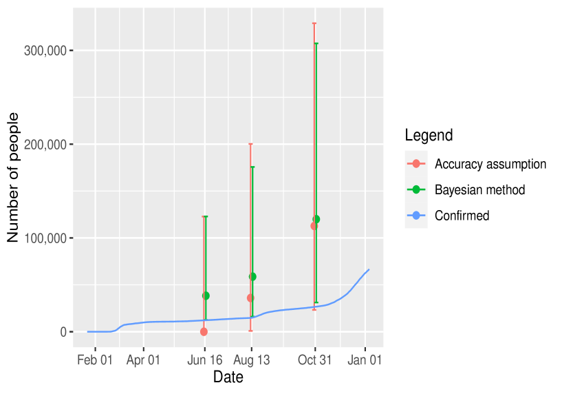
Figure 1: Dots and error bars denoted by “Bayesian method” represent the posterior mean and $\displaystyle 95\%$ credible intervals of the multiplied posterior distributions on seroprevalance parameters by the proposed Bayesian method. Dots and error bars denoted by “Accuracy assumption” represent the multiplied point estimators and the multiplied $\displaystyle 95\%$ confidence intervals of the results of statistical analysis under the accuracy assumption. The line graph denoted by “Confirmed” represents the daily cumulative confirmed cases.

Figure 1 shows that the lower bounds of interval estimation by the Bayesian method are larger than the number of confirmed cases as expected, but the other does not satisfy the inequality condition. Each upper bound of the interval estimations by the Bayesian method is smaller than the corresponding one obtained under the accuracy assumption. Under the inaccuracy assumption, the Bayesian method considers that test-positive cases may include false-negative cases, which is critical when the test-positive number is small enough. Thus, the Bayesian method makes the upper bounds shrink.

5 Discussion

In this article, we have proposed a Bayesian method with informative prior, which uses the clinical evaluation results of the plaque reduction neutralization test for analyzing data on the seroprevalence surveys in South Korea. We have compared the method with the frequentist’s method under the inaccuracy assumption and the statistical analysis under the accuracy assumption. The main advantages of the proposed method are two. First, the method allows the constrained parameter space, which has an obvious lower bound as the proportion of the cumulative confirmed cases. Second, when we consider the inaccuracy assumption, the method can provide a practically corrected estimate contrary to the frequentist’s method.

However, this study has a limitation. Each set of samples in the seroprevalence survey does not cover all the regions in South Korea. In the first survey announced on the 9th of July, the survey samples do not include those from the populations of several major cities such as Daegu, Daejeon, and Sejong. Daegu particularly was the city of the first mass outbreak in South Korea. The other surveys also do not cover all the cities. The second survey samples do not include those from Ulsan, Busan, Jeonnam, and Jeju, and for the third survey, Gwangju and Jeju are not covered.

References

- (1)
- Arora et al. (2020) Arora, R. K., Joseph, A., Van Wyk, J., Rocco, S., Atmaja, A., May, E., Yan, T., Bobrovitz, N., Chevrier, J., Cheng, M. P. et al. (2020). SeroTracker: a global SARS-CoV-2 seroprevalence dashboard, The Lancet. Infectious Diseases .
- Bickel and Doksum (2015) Bickel, P. J. and Doksum, K. A. (2015). Mathematical statistics: basic ideas and selected topics, volume I, Vol. 117, CRC Press.
- Carpenter et al. (2017) Carpenter, B., Gelman, A., Hoffman, M. D., Lee, D., Goodrich, B., Betancourt, M., Brubaker, M., Guo, J., Li, P. and Riddell, A. (2017). Stan: A probabilistic programming language, Journal of statistical software 76(1).
- Clopper and Pearson (1934) Clopper, C. J. and Pearson, E. S. (1934). The use of confidence or fiducial limits illustrated in the case of the binomial, Biometrika 26(4): 404–413.
- Diggle (2011) Diggle, P. J. (2011). Estimating prevalence using an imperfect test, Epidemiology Research International 2011.
- Gorbalenya et al. (2020) Gorbalenya, A., Baker, S., Baric, R., de Groot, R., Drosten, C., Gulyaeva, A., Haagmans, B., Lauber, C., Leontovich, A., Neuman, B. et al. (2020). The species severe acute respiratory syndrome related coronavirus: classifying 2019-nCoV and naming it SARS-CoV-2. Nat Microbiol 5: 536–544.
- Kohmer et al. (2020) Kohmer, N., Westhaus, S., Rühl, C., Ciesek, S. and Rabenau, H. F. (2020). Brief clinical evaluation of six high-throughput SARS-CoV-2 IgG antibody assays, Journal of Clinical Virology p. 104480.
-