Reproducing kernel Hilbert spaces, polynomials and the classical moment problem

Abstract

We show that polynomials do not belong to the reproducing kernel Hilbert space of infinitely differentiable translation-invariant kernels whose spectral measures have moments corresponding to a determinate moment problem. Our proof is based on relating this question to the problem of the best linear estimation in continuous time one-parameter regression models with a stationary error process defined by the kernel. In particular, we show that the existence of a sequence of estimators with variances converging to $0$ implies that the regression function cannot be an element of the reproducing kernel Hilbert space. This question is then related to the determinacy of the Hamburger moment problem for the spectral measure corresponding to the kernel.

AMS Subject Classification: 46E22, 62J05, 44A60

Keywords and Phrases: Reproducing kernel Hilbert spaces, classical moment problem, best linear estimation, continuous time regression model

1 Introduction

1.1 Main results

Let $X\!\subseteq\!\mathbb{R}^{d}$, $d\!\geq\!1$, $K\!:\!X\times X\!\to\!\mathbb{R}$ be a positive definite kernel on $X$ and define $H(K)$ as the corresponding Reproducing Kernel Hilbert Space (RKHS). We assume that $X$ has a non-empty interior and $K$ is an infinitely differentiable (on the diagonal) translation-invariant kernel so that $K(x,y)\!=\!k(x\!-\!y)$, where $k:\mathbb{R}^{d}\to\mathbb{R}$ is a non-constant positive definite function infinitely differentiable at the point $0$. Clearly, the function $k(\cdot)$ is even so that $k(u)=k(-u)$ for all $u\in\mathbb{R}^{d}$. Without loss of generality, we suppose $k(0)=1$.

It is well-known, see e.g. Corollary 4.44 in Steinwart and Christmann, (2008), that in the case of the Gaussian (squared exponential) kernel

$$k(x)=\exp\{-\lambda\|x\|^{2}\}\;\;{\rm with}\;\lambda>0,$$ (1.1)

the constant function does not belong to $H(K)$. This result has been generalized to arbitrary polynomials in Minh, (2010). The purpose of this paper is to significantly extend these results (previously only known for the case of the Gaussian kernel) to a substantially larger class of kernels.

In the main part of the paper, we consider the case $X\subset\mathbb{R}$. In this case, by Bochner’s theorem (Bochner and Chandrasekharan,, 1949), there exists a measure $\alpha$, such that the function $k$ can be represented in the form

$$k(x)=\int_{-\infty}^{\infty}e^{itx}\alpha(dt)~{}~{}\mbox{ for all }x\in X.$$ (1.2)

The measure $\alpha$ is called spectral measure. As function $k(\cdot)$ is even and $k(0)=1$, $\alpha(dt)$ is a probability measure symmetric around the point 0. The moments of this measure (in the case of their existence) will be denoted by $c_{n}=\int_{-\infty}^{\infty}t^{n}\alpha(dt)$. Since we assume $k(\cdot)$ in (1.2) is infinitely differentiable and even, we have

$$c_{n}=\int_{-\infty}^{\infty}t^{n}\alpha(dt)=\left\{\begin{array}[]{cl}(-1)^{n/2}\,k^{(n)}(0),&\mbox{ if $n$ is even}\\ 0,&\mbox{ if $n$ is odd}\\ \end{array}\right.\,,$$ (1.5)

where $k^{(n)}(0)=\frac{\partial^{n}}{\partial u^{n}}k(u)\big{|}_{u=0}$.

The classical Hamburger moment problem is to give necessary and sufficient conditions such that a given real sequence $(c_{n})_{n\in\mathbb{N}}$ is in fact a sequence of moments of a distribution $\alpha$ defined on the Borel sets of $\mathbb{R}=(-\infty,\infty)$. In particular, the sequence $(c_{n})_{n\in\mathbb{N}}$ is a sequence of moments of some distribution if and only if the Hankel matrices $(c_{i+j})_{i,j=0,\ldots,n}$ are positive semidefinite for all $n\in\mathbb{N}$; see e.g. Shohat and Tamarkin, (1943); Schmüdgen, (2017) among many others. The Hamburger moment problem is called determinate if the sequence of moments $(c_{k})_{k\in\mathbb{N}}$ determines the measure $\alpha(dt)$ uniquely.

The main results of this paper are Theorems 1.1 and 1.2 formulated below. These theorems provide sufficient conditions ensuring that the polynomials do not belong to the RKHS $H(K)$. The proofs are given in Section 2.5.

Theorem 1.1

Let $X\subset\mathbb{R}$ and assume that the spectral measure $\alpha(dt)$ in (1.2) has infinite support and no mass at the point 0. If the Hamburger moment problem for this measure is determinate, then the non-zero constant functions do not belong to the RKHS $H(K)$.

Theorem 1.2

Let $X\subset\mathbb{R}$, $m$ be a positive integer and assume that the spectral measure $\alpha(dt)$ in (1.2) has infinite support. If the Hamburger moment problem for the measure $\alpha_{m}(dt)=t^{2m}\alpha(dt)/c_{2m}$ is determinate (here, as in (1.5), $c_{2m}=\int t^{2m}\alpha(dt)$), then the RKHS $H(K)$ does not contain polynomials on $X$ of degree precisely $m$.

Theorem 1.2 can be considered as a corollary of Theorem 1.1 and therefore the result of Theorem 1.1 is more fundamental. In the very important particular case (see the sufficient condition for moment determinacy (1.3) and related discussion in Section 1.3), when the function $k(\cdot)$ is real analytic and vanishes at infinity while $X$ is bounded, $H(K)$ contains only those analytic functions that vanish at infinity. This is formally proven in Karvonen, (2021) and basically follows from the fact that if $f\in H(K)$ then $f(x)$ is a point-wise limit of the sums $\mu_{N}(x)=\sum_{i=1}^{N}w_{i}k(x_{i}-x)$ with $x_{i}\in X$, which necessarily vanish at infinity.

Combining Theorems 1.1 and 1.2 with their variations in the cases when the spectral measure $\alpha(dt)$ has finite support (see Section 3.1) and when this measure has positive mass at 0 (see Theorem 3.1), we obtain the following corollary.

Corollary 1.1

Let $X\subset\mathbb{R}$ and the Hamburger moment problem for the spectral measure $\alpha(dt)$ be determinate. Then we have the following:

• the constant functions $f(x)={\rm const}\neq 0$, $\forall x\in X$, belong to $H(K)$ if and only if $\alpha(dt)$ has a positive mass at the point 0;

• if additionally $k(\cdot)$ is a real analytic function, then $H(K)$ does not contain non-constant polynomials on $X$.

Theorems 1.1, 1.2 and Corollary 1.1 can be easily extended to the multivariate case, see Section 3.2.

1.2 Implications and related results

Gaussian process (GP) models deal with an unknown deterministic function assuming that it is a realization of Gaussian process (field) with some mean and covariance kernel, which are perhaps parameterized. The popularity of the GP model comes from its transparency, flexibility and computational tractability; it is used as a general-purpose technique to model, explore and exploit unknown functions. As a result, methods based on the GP models constitute much of the modern statistical toolkit for function approximation, interpolation and prediction (Stein,, 1999; Wendland,, 2004), integration (Briol et al.,, 2019), machine learning (Rasmussen and Williams,, 2006; Steinwart and Christmann,, 2008), space-filling (Pronzato and Zhigljavsky,, 2020), signal processing (Cambanis and Masry,, 1983), probabilistic numerics (Hennig et al.,, 2015) and global optimization (Zhigljavsky and Žilinskas,, 2021). The practical application areas of the GP model are vast, and we refer the references in the cited papers and to the work of Schulz et al., (2018), Archetti and Candelieri, (2019) among others.

Consider the common framework of GP regression (simple kriging), where the a function $f:X\to\mathbb{R}$ to be approximated ($X\subset\mathbb{R}^{d}$) is considered as a realization of a GP, say $\{Z_{x}\}_{x\in X}$, with mean zero, covariance

$$\mathbb{E}\{Z_{x}Z_{x^{\prime}}\}=\sigma^{2}\,K(x,x^{\prime}) x,x^{\prime}\in X\subset\mathbb{R}^{d}$$ for all , (1.6)

and $\sigma^{2}>0$ may be unknown; see Rasmussen and Williams, (2006) for more details. Let the kernel $K$ be strictly positive definite, $X_{N}=\{x_{1},\ldots,x_{N}\}$ be an $N$-point design consisting of distinct points $x_{i}\in X$ and $F_{N}=[f(x_{1}),\ldots,f(x_{N})]^{\top}\in\mathbb{R}^{N}$ be the vector of exact observations of $f$ at the points of $X_{N}$. The conditional process $\{Z_{x}|(X_{N},F_{N})\}_{x\in X}$ is again Gaussian with conditional mean

$$\mu_{N}(x)=F_{N}^{\top}K_{N}^{-1}b_{N}(x)$$ (1.7)

and covariance function

$$C_{N}(x,y)=K(x,x^{\prime})-b_{N}^{\top}(x)K_{N}^{-1}b_{N}(x^{\prime}),$$ (1.8)

where $K_{N}=(K(x_{i},x_{j}))_{i,j=1}^{N}\,$ and $b_{N}(\cdot)=[K(x_{1},\cdot),\ldots,K(x_{N},\cdot)]^{\top}$. Straightforward calculation shows that the conditional mean $\mu_{N}(x)$ is the best linear predictor of $f(x)$ and $\sigma^{2}\,C_{N}(x,x)$ is the corresponding mean squared prediction error at the point $x$.

GP regression is equivalent to kernel interpolation, see e.g. Scheuerer et al., (2013), Section 3.3 in Kanagawa et al., (2018) and Chapter 3 in Paulsen and Raghupathi, (2016). More precisely, the conditional mean $\mu_{N}(\cdot)$ is the minimal-norm interpolant to $f$ among all functions in $H(K)$, where we use the norm on $H(K)$ denoted below by $\|\cdot\|_{H(K)}$. This property implies in particular that if $f\in H(K)$ then $\|\mu_{N}\|_{H(K)}\leq\|f\|_{H(K)}$, where this inequality holds for any $f\in H(K)$ and any set of points $X_{N}$. If $f\notin H(K)$ then the conditional mean $\mu_{N}(\cdot)$ is still an element of $H(K)$ but its norm tends to infinity as $N$ grows and $X_{N}$ becomes denser. Therefore, there is a fundamental difference between the complexity of the approximation problem of $f$ depending on whether $f\in H(K)$ or $f\notin H(K)$. Correspondingly, properties of all other techniques based on the use of the GP model also heavily depend on whether an unknown function of interest belongs to the corresponding RKHS. We also refer to the work of Steinwart et al., (2006) and to Section 4.4 in Steinwart and Christmann, (2008) for a discussion on the importance of this issue for the learning performance of support vector machines (SVMs) in the case of the Gaussian kernel (1.1) as well as for the difficulty of deciding whether a given function $f$ belongs to the RKHS $H(K)$ for a chosen kernel $K$. In GP regression, knowing that the non-zero constant functions do not belong to the RKHS $H(K)$ is especially important as it can be used to justify omitting function centering; see, for example, Assumption 2 in Lee et al., (2016).

Assume now that the factor $\sigma^{2}$ in (1.6) is unknown and that the maximum likelihood estimator (MLE) $\widehat{\sigma^{2}_{N}}$ of $\sigma^{2}$ is constructed from the observations of the function $f$ at the points $x_{i}\in X_{N}$; see Section 3.5. If $f$ is indeed a realization of the GP with covariance (1.6), it follows by the well-known results on microergodicity (see Chapter 6 in Stein,, 1999) that $\widehat{\sigma^{2}_{N}}\to\sigma^{2}$ almost surely (a.s.) as $N\to\infty$ and $X_{N}$ becomes dense in $X$. Note, however, that such realizations do not belong to $H(K)$ a.s. and if $f\in H(K)$ then $\widehat{\sigma^{2}_{N}}\to 0$ as $N\to\infty$. This observation is a consequence of the useful relation $\widehat{\sigma^{2}_{N}}=\frac{1}{N}\|\mu_{N}\|_{H(K)}^{2}$ (see equation (3.4) in Karvonen et al.,, 2020) and the relation $\|\mu_{N}\|_{H(K)}\leq\|f\|_{H(K)}$, which has already been mentioned. This is in full agreement with Corollary 3.3 below, which states that $f\in H(K)$ if and only if $\lim_{N\to\infty}N\,\widehat{\sigma^{2}_{N}}<\infty$ (assuming $X_{N}$ becomes dense in $X$ as $N\to\infty$). Our numerical studies in Section 5 of this paper show, however, that for finite sample sizes the asymptotic behaviour of $\widehat{\sigma^{2}_{N}}$ has much less effect on uncertainty quantification in GP regression than the smoothness of the function $k(x)$ and its flatness at $x\simeq 0$.

The problem of deciding whether a given function $f$ belongs to the RKHS $H(K)$ for a chosen kernel $K$ is well-known in literature, see e.g. Section 3.4 in Paulsen and Raghupathi, (2016). This problem is well-studied in the case of kernels with finite number of derivatives, (Ritter,, 2007; Ritter et al.,, 1995; Karvonen et al.,, 2020). For infinitely differentiable kernels, only the case of Gaussian kernel (1.1) is well-understood; see Minh, (2010) for most advanced results. In a preprint citing the present paper, Karvonen, (2021) gives further new results for analytic translation-invariant kernels with $\lim_{\|x\|\to\infty}k(x)=0$.

1.3 Sufficient conditions for moment determinacy

There are many sufficient conditions for moment determinacy of probability measures, see e.g. Lin, (2017), Schmüdgen, (2017) and Stoyanov, (2013, Chapter 11). The following sufficient condition for moment determinacy of a measure $\alpha(dt)$ with moments $c_{k}$ in the Hamburger moment problem, the so-called Carleman condition, is one of the most commonly used:

$${\rm(A.1):}\;\;\;\;\;\;\;\;\;\;\;\;\;\;\;\;\;\;\;\;\;\;\;\;\;\;\;\;\;\;\;\;\;\;\;\;\;\;\;\;\;\;\;\;\;\;\;\;\sum_{n=1}^{\infty}c_{2n}^{-1/(2n)}=\infty\,.\;\;\;\;\;\;\;\;\;\;\;\;\;\;\;\;\;\;\;\;\;\;\;\;\;\;\;\;\;\;\;\;\;\;\;\;\;\;\;\;\;\;\;\;\;$$ (1.9)

Note that if a probability measure $\alpha(dt)$ has finite moments $c_{j}$ for all $j=0,1,\ldots$ and satisfies (1.9), then for any $m=0,1,\ldots$ the measure $\alpha_{m}(dt)=t^{2m}\alpha(dt)/c_{2m}$ of Theorem 1.2 with moments $\int t^{j}\alpha_{m}(dt)=c_{2m+j}/c_{2m}$ also satisfies (1.9).

Less known than (1.9) is the following sufficient condition for the moment determinacy (in the Hamburger moment problem) of a measure $\alpha(dt)$:

$${\rm(A.2):}\;\;\;\;\;\;\;\;\;\;\;\;\;\;\;\;\;\;\;\;\;\;\;\;\exists\,\varepsilon>0\;\mbox{ such that}\;\sum_{n=1}^{\infty}{|c_{n}|x^{n}\over n!}<\infty\;\;\;\mbox{for all $|x|<\varepsilon$,}\;\;\;\;\;\;\;\;\;\;\;\;\;\;\;\;\;\;$$

see Theorem 30.1 in Billingsley, (2008). This condition is clearly equivalent to the assumption (A.3): the random variable (r.v.) $\xi_{\alpha}$ with distribution $\alpha$ has moment generating function and, see Theorem 1 in Lin, (2017), to (A.4): $\limsup_{n\to\infty}\frac{1}{2n}c_{2n}^{1/(2n)}<\infty;$ this is one of the most known and easiest to verify sufficient conditions for moment determinacy. Theorem 2.13 in Wainwright, (2019) yields that the assumptions (A.2)–(A.4) are also equivalent to the assumption (A.5): the r.v. $\xi_{\alpha}$ is sub-exponential. In view of this assumption, the tail behaviour of $\alpha(dt)$ is a natural indicator of the degree of moment-determinacy of $\alpha$.

The conditions (A.2)–(A.5) are stronger than the Carleman condition (1.9) in the sense that any of them implies (1.9). A technique of constructing measures $\alpha$ satisfying the Carleman condition (1.9) but violating $\limsup_{n\to\infty}\frac{1}{2n}c_{2n}^{1/(2n)}<\infty$, and hence all other assumptions in (A.2)–(A.5), is given in Stoyanov, (2013), Section 11.9.

In view of (1.5) and symmetry of $k(\cdot)$, $|c_{n}|=|k^{(n)}(0)|$ for all integers $n=0,1,\ldots$ This yields that (A.2) coincides with the assumption that $k(\cdot)$ is a real analytic function at the point $0$, see Definition 1.1.5 and Corollary 1.1.16 in Krantz and Parks, (2002). Summarizing, if $k(\cdot)$ is a real analytic at $0$, then the corresponding spectral measure $\alpha(dt)$ is moment-determinant in the Hamburger sense. It is not difficult, however, to construct moment-determinant (in the Hamburger sense) spectral measures $\alpha(dt)$ which do not satisfy (A.2); see Sections 11.9 and 11.10 in Stoyanov, (2013). For such measures, the corresponding functions $k(\cdot)$ are symmetric, positive definite and infinitely differentiable but not real analytic at $0$. Nevertheless, for practical purposes the class of functions which are symmetric, positive definite and real analytic can be considered as the main class of functions $k(\cdot)$, for which the corresponding spectral measures are moment determinant in the Hamburger sense. Note also that if the function $k(\cdot)$ is real analytic then all functions in $H(K)$ have to be analytic too; see Sun and Zhou, (2008).

Let us give four examples of kernels $K(x,y)=\sigma^{2}k(x-y)$ whose spectral measures $\alpha(dt)$ satisfy the Carleman condition (1.9) and hence assumptions of Theorems 1.1, 1.2 and Corollary 1.1 (we will return to these kernels in Sections 4 and 5). The spectral density corresponding to the spectral measure $\alpha(\cdot)$ will be denoted by $\varphi(\cdot)$, so that $\alpha(dt)=\varphi(t)dt$. In examples (E.1)–(E.4) below, we also provide asymptotic expressions for $C_{N}(\alpha)=\sum_{n=1}^{N}c_{2n}^{-1/(2n)}$. In view of (1.9), the rate of divergence of $C_{N}(\alpha)$ (as $N\to\infty$) can also be used to characterize the degree of moment-determinacy of $\alpha$ (additionally to the tail behaviour of $\alpha$).

• Gaussian kernel: $k(x)=\exp\{-\lambda x^{2}/2\}$, $\varphi_{{\lambda}}(t)=\frac{1}{\sqrt{2\pi\lambda}}\exp\{-t^{2}/(2\lambda)\}$ ($t\in\mathbb{R}$), $c_{2n}=\lambda^{n}(2n-1)!!$, $C_{N}(\alpha)=\sum_{n=1}^{N}c_{2n}^{-1/(2n)}=\sqrt{N/\lambda}(1+o(1)),\,N\to\infty$.

• Cauchy kernel: $k(x)=1/(1+x^{2}/\lambda^{2})$, $\varphi_{{\lambda}}(t)=\frac{\lambda}{2}\exp\{-{\lambda}|t|\}$ ($t\in\mathbb{R}$), $c_{2n}=\lambda^{-n}(2n)!$, $c_{2n}^{-1/(2n)}=e\sqrt{\lambda}/n+o(1/n)$, so that $C_{N}(\alpha)=e\sqrt{\lambda}\log N(1+o(1))$ as $N\to\infty$.

• The kernel whose spectral density is a symmetric Beta-density:
  ${\varphi}_{a}(t)={2^{-2a-1}}(1-t^{2})^{a}/{B(a+1,a+1)}$ with $a>-1$ and $t\in[-1,1]$.
  Here we have $C_{N}(\alpha)={\rm const}\cdot N(1+o(1))$ as $N\to\infty$.

• $k(x)=\cos(\lambda x)$ with $\lambda\neq 0$; here the spectral measure $\alpha$ is concentrated at $\pm\lambda$ with masses $1/2$ yielding $c_{2n}=\lambda^{2n}$, $c_{2n}^{-1/(2n)}=1/\lambda$ and $C_{N}(\alpha)=N/\lambda$ for all $N$.

1.4 Main steps in the proofs and the structure of the remaining part of the paper

Section 2 is devoted to proving Theorems 1.1 and 1.2; the proofs are given in several steps. The main idea in our approach is to relate the problem of interest to properties of the best linear unbiased estimate (BLUE) in linear regression models, which will be worked out in Sections 2.1 and 2.2. Sections 2.3 and 2.4 provide different characterizations of the moment determinacy of spectral measures and finally the proofs will be completed in Section 2.5. We now explain the different steps in more detail.

In Section 2.1 we consider a one-parameter linear regression model $y(x)\!=\!\theta f(x)\!+\!\varepsilon(x)$ with $\mathbb{E}\varepsilon(x)\varepsilon(x^{\prime})\!=\!K(x,x^{\prime})$ and a regression function $f\!\in\!H(K)$ and show that in this case $\hat{\theta}_{BLUE}$, the BLUE of $\theta$, exists and its variance is strictly positive, see Lemma 2.1. We also show that in the case $f\!\notin\!H(K)$, the BLUE does not exist and establish in Lemma 2.2 that for proving $f\!\notin\!H(K)$, it is sufficient to construct a sequence of linear unbiased estimators $\hat{\theta}_{n}$ of the unknown parameter with variances tending to $0.$ Such a sequence is constructed in Section 2.2 for the location scale model and an explicit expression for the variance of these estimators in terms of the ratio of determinants

$${\rm var}(\hat{\theta}_{n})=\frac{{\rm det}(c_{2(i+j)})_{i,j=0}^{n}}{{\rm det}(c_{2(i+j)})_{i,j=1}^{n}}\,$$ (1.10)

of Hankel-type matrices of the moments of the spectral measure is derived in Lemma 2.4. In Section 2.3 we establish several properties of moment-determinant symmetric measures which we use in Section 2.4 for building up an equivalence between the moment determinacy of the spectral measures and the statement that the sequence (1.10) converges to zero. This is arguably the most important step in the proof of both theorems (see Lemma 2.7). Finally, these results are combined in the proofs of Theorem 1.1 and 1.2 in Section 2.5.

In Section 3 we consider several extensions and interpretations of the main results. In Section 3.1 we consider spectral measures with finite support, while Section 3.2 discusses the multivariate case. This discussion is continued in Sections 3.3–3.5, where we also consider general metric spaces. In Section 3.3 we explain a technique of characterizing the inclusion $f\in H(K)$ via suitable discretization of the set $X$ and show that $1/\|f\|_{H(K)}$ is the limit of variances of the related discrete BLUEs. These results are used in Section 3.4, where we prove that the constant function belongs to $H(K)$ if and only if the spectral measure has positive mass at $0$. In Section 3.5 we show that the problem of parameter estimation in a one-parameter regression model is equivalent to the problem of estimating the variance of a Gaussian process (field). Thus we are able to relate our findings to the estimation problems considered in Xu and Stein, (2017) and Karvonen et al., (2020). In Section 3.6 we return to the one-dimensional case and give an interpretation of Theorem 1.1 in terms of the $L_{2}$-error of the best approximation of a constant function by polynomials of the form $a_{1}t^{2}+a_{1}t^{4}+\ldots+a_{n}t^{2n}$.

In Section 4, for two specific classes of kernels we derive explicit results on the rates of convergence to $0$ of the ratio of determinants (1.10). In the case of Gaussian kernel (1.1), we detail and improve one of the asymptotic expansions of Theorem 3.3 in Xu and Stein, (2017). Finally, in Section 5 we discuss results of a numerical study for uncertainty quantification in GP regression in relation to the theoretical results of this paper.

2 Parameter estimation, moment determinacy and proofs of main results

2.1 BLUE in a one-parameter regression model

Consider a one-parameter regression model with stationary correlated errors:

$$y(x)\!=\!\theta f(x)\!+\!\varepsilon(x) x\!\in\!X \mathbb{E}\varepsilon(x)\!=\!0, \,\mathbb{E}\varepsilon(x)\varepsilon(x^{\prime})\!=\!k(x\!-\!x^{\prime})$$, , . (2.1)

Here $\theta$ is a scalar parameter, $f\!:\!X\!\to\!\mathbb{R}$ is a given regression function and $k(\cdot)$ is an infinitely differentiable positive definite function with $k(0)=1$ making the kernel $K(\cdot,\cdot)$ defined by $K(x,y)=k(k-y)$ an infinitely differentiable correlation kernel. For constructing estimators of the parameter $\theta$, the observations of the process $\{y(x)|x\in X\}$ along with observations of all of its derivatives $\{y^{(k)}(x)|x\in X\}$, $k=1,2,\ldots$, can be used.

An estimator $\hat{\theta}$ for the parameter $\theta$ is called linear, if it is a linear function of the observations (in our case of the process and its derivatives). An unbiased estimator satisfies $\mathbb{E}[\hat{\theta}]=\theta$ for all $\theta$. The best linear unbiased estimator (BLUE) of $\theta$ is defined as an unbiased estimator $\hat{\theta}_{BLUE}$ such that $\mbox{var}(\hat{\theta}_{BLUE})\leq\mbox{var}(\hat{\theta})$, where $\hat{\theta}$ is any linear unbiased estimator of $\theta$. If the kernel $K$ is differentiable and the BLUE exists, then for its computation all available derivatives of $y(x)$ are used, see Dette et al., (2019). In general, the BLUE may not exist but the next lemma shows that it does exist when $f\in H(K)$.

Lemma 2.1

If $f\in H(K)$, then the BLUE $\hat{\theta}_{BLUE}$ in model (2.1) exists and

$$\mbox{\rm var}(\hat{\theta}_{BLUE})=1/\|f\|_{H(K)}>0.$$

The statement of lemma follows from Theorem 6C (p. 975) of Parzen, (1961). Formally, only the case $X=[0,1]$ is considered in Parzen, (1961), but Parzen’s proof does not use the structure of $X$ and is therefore valid for a general metric space $X$.

Lemma 2.2

If there exists a sequence of linear unbiased estimators $(\hat{\theta}_{n})_{n\in\mathbb{N}}$ of $\theta$ in model (2.1) such that ${\rm var}(\hat{\theta}_{n})\to 0$ as $n\to\infty$, then $f\notin H(K)$.

Proof. Assume that $f\in H(K)$. By Lemma 2.1, the continuous BLUE $\hat{\theta}_{BLUE}$ exists and var$(\hat{\theta}_{BLUE})=1/\|f\|_{H(K)}>0$. From the definition of the BLUE, ${\rm var}(\hat{\theta}_{n})\geq{\rm var}(\hat{\theta}_{BLUE})>0$ for all $n\in\mathbb{N}$. We have arrived at a contradiction and hence $f\notin H(K)$. $\Box$

2.2 A family of estimators $\hat{\theta}_{n}$ in the location scale model

Consider the location scale model

$$y(x)\!=\!\theta\!+\!\varepsilon(x)\,,\;x\!\in\!X\subset\!\mathbb{R},\;\;\mathbb{E}\varepsilon(x)\!=\!0,\;\mathbb{E}\varepsilon(x)\varepsilon(x^{\prime})\!=\!k(x\!-\!x^{\prime}),$$ (2.2)

where $k(\cdot)$ is an infinitely differentiable at 0 positive definite function. Choose any interior point $x_{0}\in X$ and set $\varepsilon_{0}=\varepsilon(x_{0})$. For construction of the estimator $\hat{\theta}_{n}$, which we will apply in Lemma 2.2, we use the following $n+1$ observations: the observation $y(x_{0})=\theta+\varepsilon_{0}\,$ at the point $x_{0}$ and $n$ mean-square derivatives of the process $y$ at the point $x_{0}$:

$$\varepsilon_{j}=y^{(j)}(x_{0})=\frac{d^{j}y(x)}{dx^{j}}\bigg{|}_{x=x_{0}}=\frac{d^{j}\varepsilon(x)}{dx^{j}}\bigg{|}_{x=x_{0}}\,,\;\;\;\;j=2,4,\ldots,2n\,.$$ (2.3)

As discussed in Section 1.3, for the main class of kernels of interest, the RKHS $H(K)$ is a subset of analytic functions. If we observe $y(x)$ everywhere on [0,1], then, since $f\in H(K)$ and $\varepsilon(x)$ are analytic, we also know all $y^{(k)}(x)$ for all $x\in[0,1]$ and any integer $k\geq 0$. Again, because of the analyticity, observing $y(x)$ everywhere on $X=[0,1]$ is the same as observing $y^{(k)}(x)$ for any $x\in[0,1]$ and any integer $k\geq 0$. This yields that in practice we do not need to directly observe $y^{(k)}(\cdot)$ for constructing estimators of $\theta$.

The following result provides a necessary and sufficient condition for the existence of the derivatives. For a proof, see page 164 (Section 12) in Yaglom, (1986).

Lemma 2.3

Let $x_{0}$ be an interior point of $X$. The mean-square derivative $\varepsilon_{j}={d^{j}\varepsilon(x)}/{dx^{j}}\big{|}_{x=x_{0}}$ of the stationary process $\{\varepsilon(x)|x\in X\}$ in (2.2) at the point $x_{0}$ exists if and only if $c_{2j}<\infty$, where

$$c_{2j}=\int_{-\infty}^{\infty}t^{2j}\alpha(dt)=(-1)^{j}\frac{\partial^{2j}}{\partial u^{2j}}k(u)\bigg{|}_{u=0}$$ (2.4)

is the $2j$-th moment of the spectral measure $\alpha$ corresponding to the kernel $k$ in Bochner’s theorem.

As we have assumed that the kernel $k(\cdot)$ is infinitely differentiable at 0, all moments $c_{j}$ ($j=0,1,\ldots$) exist. As an immediate consequence of the existence of all moments and the representation (1.2), for the random variables $\varepsilon_{j}$ defined in (2.3), we obtain by Lemma 2.3

$$\mathbb{E}\varepsilon_{i}\varepsilon_{j}=\frac{\partial^{i+j}}{\partial x^{i}y^{j}}k(x-y)\bigg{|}_{x,y=x_{0}}=(-1)^{i+j}\frac{\partial^{i+j}}{\partial u^{i+j}}k(u)\bigg{|}_{u=0}=c_{i+j}\,.$$ (2.5)

for all $i,j=0,1,\ldots$ Note that all derivatives ${\partial^{m}}/{\partial u^{m}}k(u)\big{|}_{u=0}$ of odd order $m$ vanish as the function $k(\cdot)$ is symmetric around the point $0$.

Next, we introduce the random variables $\delta_{i}=(-1)^{i}\varepsilon_{2i}$, $i=0,1,\ldots$. The observations (2.3) used for constructing the discrete BLUE in model (2.2) can then be rewritten as

$$y_{0}=y(x_{0})=\theta+\varepsilon_{0},\;y_{1}=y^{(2)}(x_{0})=\delta_{1},\;\ldots,\;y_{n}=y^{(2n)}(x_{0})=\delta_{n}.$$

Moreover, the covariance matrix of the vector $(\delta_{0},\delta_{1},\ldots,\delta_{n})^{\top}$ is the Hankel matrix

$$C_{n}=\left(\mathbb{E}\delta_{i}\delta_{j}\right)_{i,j=0}^{n}=(c_{2(i+j)})_{i,j=0}^{n}\,,$$ (2.6)

where $c_{2},\ldots,c_{2n}$ are the moments defined in (2.4).

Assume that the spectral measure $\alpha(dt)$ has infinite support. In this case, the matrices $C_{n}$ are positive definite for all $n=0,1,\ldots$ (see, for example, Proposition 3.11 in Schmüdgen,, 2017) and the discrete BLUE is obtained as

$$\hat{\theta}_{n}=\frac{e_{0,n}^{\top}C_{n}^{-1}Y_{n}}{e_{0,n}^{\top}C_{n}^{-1}e_{0,n}},$$ (2.7)

where $Y_{n}=(y_{0},y_{1},\ldots,y_{n})^{\top}$ and $e_{0,n}=(1,0,\ldots,0)^{\top}\in\mathbb{R}^{n+1}$ denotes the first coordinate vector in $\mathbb{R}^{n+1}$.

Lemma 2.4

The variance of the estimator (2.7) is

$${\rm var}(\hat{\theta}_{n})=\frac{1}{e_{0,n}^{\top}C_{n}^{-1}e_{0,n}}=\frac{H_{n}}{G_{n}}\,,$$ (2.8)

where $H_{n}$ and $G_{n}$ are the determinants

$$H_{n}={\rm det}\left(C_{n}\right)={\rm det}\left[\left(c_{2(i+j)}\right)_{i,j=0}^{n}\right]\,,\;\;\;G_{n}={\rm det}\left[\left(c_{2(i+j)}\right)_{i,j=1}^{n}\right]\,.$$ (2.9)

Proof. The expression (2.8) follows from the standard formula ${\rm var}(\hat{\theta}_{n})=1/(e_{0,n}^{\top}C_{n}^{-1}e_{0,n})$ for the variance of the BLUE and Cramér’s rule for computing elements of a matrix inverse; in our case, $e_{0,n}^{\top}C_{n}^{-1}e_{0,n}$ coincides with the top-left element of the matrix $C_{n}^{-1}$. $\Box$

Observing Lemma 2.2 we conclude that a non-vanishing constant function does not belong to $H(K)$ if $\lim_{n\to\infty}{H_{n}}/{G_{n}}=0.$ In the following sections we relate this condition to the moment determinacy of the spectral measure.

Remark 2.1

Let us briefly consider the case where the spectral measure has a positive mass at the point $0$. Consider the location scale model (2.2) and let

$${\alpha}_{\gamma}(dt)=(1-\gamma){\alpha}(dt)+\gamma\delta_{0}(dt)\,$$ (2.10)

denote the spectral measure corresponding to a nonnegative definite and symmetric kernel $k_{\gamma}$, where $0<\gamma<1$, $\delta_{0}$ is the Dirac measure at the point $0$ and $\alpha(dt)$ is a symmetric probability measure on $\mathbb{R}$ with no mass at 0. The measure ${\alpha}_{\gamma}(dt)$ is symmetric around the point $0$ with even moments $\tilde{c}_{0}=1$ and

$$\tilde{c}_{2j}=(1-\gamma)c_{2j}\,,\;\;j=1,2,\ldots$$

Recall the definition of the matrix $C_{n}$ in (2.6) and define the matrices

$$\tilde{C}_{n}=(\tilde{c}_{2(i+j)})_{i,j=0}^{n}=\gamma e_{0,n}e_{0,n}^{\top}+(1-\gamma)C_{n}$$

and the corresponding determinants

$$\tilde{H}_{n}={\rm det}\,\tilde{C}_{n}\,,\;\;\;\tilde{G}_{n}={\rm det}\left[\left(\tilde{c}_{2(i+j)}\right)_{i,j=1}^{n}\right]=(1-\gamma)^{n}G_{n}\,,$$

where $G_{n}$ is defined in (2.9). Using standard formulas of linear algebra we obtain

$$\tilde{H}_{n}={\rm det}\,[\gamma e_{0,n}e_{0,n}^{\top}+(1-\gamma)C_{n}]=(1-\gamma)^{n}\left[(1-\gamma)+\gamma e_{0,n}^{\top}C_{n}^{-1}e_{0,n}\right]\,H_{n}\,.$$

In accordance with (2.8), the variance of $\tilde{\theta}_{n}$, the BLUE of $\theta$ constructed similarly to $\hat{\theta}_{n}$ but for the spectral measure ${\alpha}_{\gamma}(dt)$, is given by

$${\rm var}(\tilde{\theta}_{n}) = \frac{1}{e_{0,n}^{\top}\tilde{C}_{n}^{-1}e_{0,n}}=\frac{\tilde{H}_{n}}{\tilde{G}_{n}}=\frac{H_{n}}{G_{n}}\left[(1-\gamma)+\gamma e_{0,n}^{\top}C_{n}^{-1}e_{0,n}\right]$$

$$= {\rm var}(\hat{\theta}_{n})[(1-\gamma)+\gamma/{\rm var}(\hat{\theta}_{n})]=(1-\gamma){\rm var}(\hat{\theta}_{n})+\gamma>0\,.$$

This implies that ${\rm var}(\tilde{\theta}_{n})$ cannot converge to $0$ and Lemma 2.2 is not applicable if the spectral measure has a positive mass at the point $0$.
In Theorem 3.1 of Section 3.4 we will prove that for any compact set $X\subset\mathbb{R}^{d}$ the constant functions indeed belong to $H(K)$, if the spectral measure has a positive mass at the point $0$.

2.3 Moment-determinacy of the spectral measure

Consider the spectral measure $\alpha$ introduced in equation (1.2). As a spectral measure, $\alpha$ is a symmetric measure (around $0$) on the real line and we have assumed that $\alpha$ does not have a positive mass at the point $0$. Moreover, we have assumed $k(0)=1$ making $\alpha$ a probability distribution. In the following we relate $\alpha$ to a (unique) measure on the nonnegative axis $[0,\infty)$. Loosely speaking, if a real valued random variable $\xi$ has distribution $\alpha(dt)$, then $\alpha_{+}(dt)$ is the distribution of the random variable $\xi^{2}$. In the opposite direction, if the nonnegative random variable $\eta$ has distribution $\alpha_{+}(dt)$, then $\pm\sqrt{\eta}$ has distribution $\alpha(dt)$, where $\pm$ denotes a random sign.

For a more formal construction we follow the arguments in Section 3.3 of Schmüdgen, (2017) and denote by ${\cal B}$ the Borel sigma field on $\mathbb{R}$, define $\tau:\mathbb{R}\to[0,\infty);\tau(x)=x^{2}$ and $\kappa:[0,\infty)\to\mathbb{R}$, $\kappa(x)=\sqrt{x}$. Then for any symmetric (Radon) measure $\alpha$ on ${\cal B}$, the measure $\alpha_{+}$ defined by

$$\alpha_{+}(B)=\alpha(\tau^{-1}(B))\qquad B\in{\cal B}\cap[0,\infty)$$ (2.11)

defines a measure on ${\cal B}\cap[0,\infty)$. Conversely, if $\alpha_{+}$ is a measure on ${\cal B}\cap[0,\infty)$, then

$$\alpha(B)=\frac{1}{2}\big{(}\alpha_{+}(\kappa^{-1}(B))+\alpha_{+}((-\kappa)^{-1}(B))\big{)}$$ (2.12)

defines a symmetric measure on ${\cal B}$. It now follows from Theorem 3.17 in Schmüdgen, (2017) that the relations (2.11) and (2.12) define a bijection from the set of all symmetric measures on $\mathbb{R}$ onto the set of all measures on $[0,\infty)$.

The even moments of a symmetric probability measure $\alpha$ on ${\cal B}$ are related to the moments of the measure $\alpha_{+}$ from (2.11) by

$$c_{2j}=\int_{-\infty}^{\infty}t^{2j}\alpha(dt)=2\int_{0}^{\infty}t^{2j}\alpha(dt)=\int_{0}^{\infty}t^{j}d\alpha_{+}(t)=b_{j},\;\;j\in\mathbb{N}\;,$$ (2.13)

and as a consequence the determinants $H_{n}$ and $G_{n}$ in (2.9) can be represented as

$$H_{n}={\rm det}\left[\left(b_{i+j}\right)_{i,j=0}^{n}\right]\,,\;\;\;G_{n}={\rm det}\left[\left(b_{i+j}\right)_{i,j=1}^{n}\right]\,.$$ (2.14)

Similarly to the case of the Hamburger moment problem, the Stieltjes moment problem is to give necessary and sufficient conditions such that a real sequence $(b_{j})_{j\in\mathbb{N}}$ is in fact a sequence of moments of a measure $\alpha_{+}(dt)$ on the Borel sets of $[0,\infty)$; that is $b_{j}=\int_{0}^{\infty}t^{j}d\alpha_{+}(t)$ for all $j\in\mathbb{N}_{0}$. The Stieltjes moment problem is determinate if the sequence of moments $(b_{j})_{j\in\mathbb{N}}$ determines the measure $\alpha_{+}(dt)$ uniquely. For a proof of the following result, which relates the Hamburger and Stieltjes moment problem, see Heyde, (1963, Lemma 1), Schmüdgen, (2017, Proposition 3.19) and Stoyanov, (2013, Sect. 11.10).

Lemma 2.5

Let $\alpha$ be a symmetric probability measure on ${\cal B}$. The Hamburger moment problem for $\alpha$ is determinate if and only if the Stieltjes moment problems for the measure $\alpha_{+}$ defined by (2.11) is determinate.

Note that for the equivalence in Lemma 2.5 to hold, the assumption that $\alpha$ does not have mass at $0$ is not required. This assumption, however, is needed in the next lemma.

Lemma 2.6

Let $\alpha$ be a symmetric probability measure on ${\cal B}$ with no mass at the point $0$. The Hamburger moment problem for $\alpha$ is determinate if and only if the Hamburger moment problem for the measure $\alpha_{+}$ defined by (2.11) is determinate.

Proof. Using the result of Theorem A in Heyde, (1963) (see also (Stoyanov,, 2013, p.113) and (Schmüdgen,, 2017, Remark 2.12)), if the Stieltjes moment problems for the measure $\alpha_{+}$ is determinate and the measure $\alpha_{+}$ has no mass at 0, then the Hamburger moment problems for this measure is also determinate. From Lemma 2.5, the required equivalence follows. $\Box$

2.4 Relating moment-determinacy of the measure $\alpha_{+}$ to ${\rm var}(\hat{\theta}_{n})$

Lemma 2.7

Let $\alpha$ be a symmetric probability measure on ${\cal B}$ with infinite support and no mass at the point $0$. The Hamburger moment problem for the measure $\alpha_{+}$ defined by (2.11) is determinate if and only if $H_{n}/G_{n}\to 0$ as $n\to\infty$, where the determinants $H_{n}$ and $G_{n}$ are defined in (2.14).

Proof. (i) Assume that the moment problem for the measure $\alpha_{+}$ is determinate. Let $\mathcal{P}_{n}$ denote the class of all polynomials of degree $n$ and define

$$\rho_{n}(t_{0})=\min\left\{\int_{\mathbb{R}}|P_{n}(t)|^{2}\alpha_{+}(dt)\mid P_{n}\in\mathcal{P}_{n},P_{n}(t_{0})=1\right\}$$

for any $t_{0}\in\mathbb{R}$, which is not a root of the $n$th orthogonal polynomial with respect to the measure $\alpha_{+}$ (see equation (2.26) in Lemma 2.11 of Shohat and Tamarkin,, 1943). Then

$$\lim_{n\to\infty}\rho_{n}(t_{0})=:\rho(t_{0})$$

exists, by Theorem 2.6 in Shohat and Tamarkin, (1943). As the point $0$ is not a support point of the measure $\alpha_{+}$ and all roots of the orthogonal polynomials with respect to the measure $\alpha_{+}$ are located in supp$(\alpha_{+})\subset(0,\infty)$ we have from Corollary 2.6 in Shohat and Tamarkin, (1943) that

$$\rho(0)=\lim_{n\to\infty}\rho_{n}(0)=0.$$

Moreover, by the discussion on p. 72 (middle of the page) in Shohat and Tamarkin, (1943) it follows that $\rho_{n}(0)$ is exactly the ratio $H_{n}/G_{n}$, where $H_{n}$ and $G_{n}$ are the determinants in (2.14). Hence the moment determinacy for the measure $\alpha_{+}$ implies $H_{n}/G_{n}\to 0$ as $n\to\infty$.

(ii) To prove the converse, assume that $H_{n}/G_{n}\to 0$ as $n\to\infty$. Let $\lambda_{n}$ be the smallest eigenvalue of the matrix $C_{n}$. Theorem 1.1 in Berg et al., (2002) states that the condition

$$\lim_{n\to\infty}\lambda_{n}=0$$

is necessary and sufficient for the moment-determinacy of the measure $\alpha_{+}$.

From the definition of $\lambda_{n}$ as the smallest eigenvalue of the matrix $C_{n}$ and the representation (2.8) it follows

$$\lambda_{n}\leq{1\over e_{0,n}^{\top}C_{n}^{-1}e_{0,n}}=\frac{H_{n}}{G_{n}}=\rho_{n}(0)$$

for all $n\in\mathbb{N}$ (see also a related discussion in Berg et al.,, 2002). Therefore, $H_{n}/G_{n}\to 0$ as $n\to\infty$ implies $\lambda_{n}\to 0$ as $n\to\infty$ and this yields the moment determinacy of the measure $\alpha_{+}$. $\Box$

2.5 Proof of Theorem 1.1 and  1.2

Proof of Theorem 1.1. Use Lemma 2.2 with the estimator defined in (2.7). By Lemma 2.4 the variance of this estimator is given by (2.8). From Lemma 2.7, the determinacy of the measure $\alpha_{+}$ is equivalent to ${\rm var}(\hat{\theta}_{n})\to 0$ as $n\to\infty$. By Lemma 2.5, this is also equivalent to the moment determinacy of the spectral measure $\alpha$. $\Box$

Proof of Theorem 1.2. Assume that the function $f$ in (2.1) is a polynomial of degree $m\!\geq\!1$. Take $m$ derivatives of both sides in (2.1). The model (2.1) thus reduces to $\tilde{y}(x)=\tilde{\theta}+\tilde{\varepsilon}(x)$, $x\in X$, where $\tilde{\theta}$ is the new parameter, $\tilde{y}(x)={y}^{(m)}(x)$ are new observations and $\tilde{\varepsilon}={\varepsilon}^{(m)}$ is the new error process. From (2.178) in Yaglom, (1986), the autocovariance function of the process $\{{\varepsilon}^{(m)}(x)|x\in X\}$ is given by

$$\mathbb{E}\varepsilon^{(m)}(x)\varepsilon^{(m)}(x^{\prime})={k}_{m}(x-x^{\prime})\;\;{\rm with}\;\;{k}_{m}(x)=(-1)^{m}{k}^{(2m)}(x).$$

From (1.2), the spectral measure associated with the kernel ${k}_{m}(x-x^{\prime})$ is $\alpha_{m}(dt)=t^{2m}\alpha(dt)/c_{2m}$. Hence, the statement for the case when $f$ is a polynomial of degree $m\geq 1$ is reduced to the case of the constant function proved in Theorem 1.1; this theorem is applicable as the measure $\alpha_{m}(dt)$ does not have mass at 0 for any $m\geq 1$. $\Box$

3 Extensions of Theorems 1.1 and 1.2 and further discussion

In this section we discuss several extensions of the results derived in Sections 1 and 2. In particular, we consider spectral measures with positive mass at the point $0$ and extends the results to the multivariate case. Moreover, we briefly indicate a relation of our results to the optimal approximation of a constant function by polynomials with no intercept.

3.1 Spectral measures with finite support

If the spectral measure $\alpha(dt)$ in (1.2) has finite support, say ${\cal T}=\{\pm t_{1},\ldots,\pm t_{m}\}$ with $m\geq 1$ and $0<t_{1}<\ldots<t_{m}$, then the matrices $C_{n}$ in (2.6) are invertible for $n\leq m-1$ but

$${\rm det}(C_{n})={\rm det}(c_{2(i+j)})_{i,j=0}^{n}=0~{}\mbox{ for }~{}n\geq m.$$ (3.1)

Consequently, observing Lemma 2.4 we have in this case

$$\mbox{var}(\hat{\theta}_{n})=0\quad\quad\mbox{for }n=m,m+1,\ldots$$

Therefore, by Lemma 2.2 a non-vanishing constant function does not belong to $H(K)$ if the corresponding spectral measure has finite support.

The relation (3.1) follows, observing the representation

$$C_{n}=2\sum_{i=1}^{m}w_{i}g(t_{i})g^{\top}(t_{i})\in\mathbb{R}^{(n\!+1)\times(n\!+\!1)}$$

where $g(t)=(1,t^{2},\ldots,t^{2n})^{\top}$ and $w_{1},\ldots,w_{m}$ are the masses of the measure $\alpha$ at the points $t_{1},\ldots,t_{m}$. As $C_{n}$ is a sum of rank one matrices, it is singular whenever $n>m-1$. On the other hand, in the case $m=n+1$ we have by the Vandermond determinant formula

$${\rm det}\ C_{n}=\prod^{n+l}_{i=1}(2w_{i})\prod_{1\leq i<j\leq n+1}(t^{2}_{i}-t^{2}_{j})^{2}>0~{},$$

which shows that $C_{n}$ is nonsingular. Finally, if $m\geq n+1$ we have (in the Loewner ordering)

$$C_{n}\geq 2\sum_{i=1}^{n+1}w_{i}g(t_{i})g^{\top}(t_{i})$$

where the matrix on the right-hand side is positive definite.

3.2 Multivariate case

Consider the location scale model (2.2) but assume that $X$ is a subset of $\mathbb{R}^{d}$ with non-empty interior. Extensions of Theorems 1.1 and 1.2 to the multivariate case, when $d>1$, essentially follow from the one-dimensional results because it is sufficient to use derivatives of the process $\{y(x);x\in X\}$ with respect to one variable for construction of estimators $(\hat{\theta}_{n})_{n\in\mathbb{N}}$ and subsequent application of Lemma 2.2. In the following discussion we consider two cases for the kernel $K(x,x^{\prime})$ using the notation $x=(x_{1},\ldots,x_{d})^{\top}$, $x^{\prime}=(x_{1}^{\prime},\ldots,x_{d}^{\prime})^{\top}$ and $t=(t_{1},\ldots,t_{d})^{\top}$. We also denote by ${x}_{(i)},x^{\prime}_{(i)}$ and ${t}_{(i)}\in\mathbb{R}^{d-1}$ the vectors $x,x^{\prime}$ and $t$ with $i$-th component removed, respectively.

Case 1: Assume that $K$ is a product kernel, that is

$$K(x,x^{\prime})=\prod_{j=1}^{d}K_{i}(x_{j},x_{j}^{\prime})\,,$$ (3.2)

where for all $j=1,\ldots,d$ the kernel $K_{j}$ (defined on a subset of $\mathbb{R}^{2}$) satisfies $K_{j}(x_{j},x_{j}^{\prime})=k_{j}(x_{j}-x_{j}^{\prime})$ and $k_{j}$ is a non-constant positive definite function infinitely differentiable at the point $0$. Denote by $\alpha_{j}(dt_{j})$ the spectral measure for $k_{j}$ and define $\alpha(dt)=\alpha_{1}(dt_{1})\cdots\alpha_{d}(dt_{d})$. To construct the sequence of estimators $(\hat{\theta}_{n})_{n\in\mathbb{N}}$ for the application of Lemma 2.2, we can use the derivatives with respect to the $i$-th coordinate for any $i$. Therefore, Corollary 1.1 can be generalized as follows.

Corollary 3.1

Assume that $X\subset\mathbb{R}^{d}$ and the kernel $K$ has the form (3.2). Then we have the following:

• If the measure $\alpha$ has a positive mass at the point $0$, then the constant functions belong to $H(K)$.

• If for at least one $i\in\{1,\ldots,d\}$ the Hamburger moment problem for the measure $\alpha_{i}(\cdot)$ is determinate and the measure $\alpha_{i}$ does not have a positive mass at the point $0,$ then any non-vanishing constant function does not belong to $H(K)$.

• If for at least one $i\in\{1,\ldots,d\}$ the Hamburger moment problem for the measures $t_{i}^{2m}\alpha_{i}(dt_{i})/c_{2m}$ is determinate for all $m=0,1,\ldots$, then $H(K)$ does not contain non-constant polynomials on $X$.

Note that the set $X$ in Corollary 3.1 does not have to be a product of one-dimensional sets. Moreover, we also point out that the assumption (3.2) can be generalized to kernels of the form

$$K(x,x^{\prime})=k_{i}(x_{i}-x_{i}^{\prime}){K}_{(d-1)}({x}_{(i)},x^{\prime}_{(i)}),$$

where ${K}_{(d-1)}(\cdot,\cdot)$ is a positive definite and suitably differentiable kernel on $\mathbb{R}^{d-1}\times\mathbb{R}^{d-1}$ and $k_{i}$ is a non-constant positive definite function infinitely differentiable at the point $0$.

Case 2: The kernel $K$ satisfies

$$K(x,x^{\prime})=k(x-x^{\prime}),$$

where $k$ is a positive definite function on $\mathbb{R}^{d}$. Consider the spectral measure $\alpha(dt)$ corresponding to $k$ by Bochner‘s theorem, that is

$$k(x)=\int_{\mathbb{R}^{d}}e^{i(t_{1}x_{1}+\ldots+t_{d}x_{d})}\alpha(dt)~{},$$ (3.3)

and denote by

$$\alpha_{i}(B)=\int_{\mathbb{\mathbb{R}}^{d}}I_{B}(t_{i})\alpha(dt)~{},~{}~{}B\in\mathcal{B},$$

the $i$th the marginal distribution of the measure $\alpha$ ($i=1,\ldots,d$), where $I_{B}$ denotes the indicator function of the set $B$. In this case, we can generalize Corollary 1.1 as follows.

Corollary 3.2

If the spectral measure $\alpha(dt)$ does not have a positive mass at the point $0$ and if for at least one $i\in\{1,\ldots,d\}$ the Hamburger moment problems for the measures proportional to $t^{2m}\alpha_{i}(dt_{i})$ are determinate for all $m=0,1,\ldots$, then $H(K)$ does not contain non-vanishing polynomials.

The case when the spectral measure has positive mass at the point $0$ is treated similarly in one-dimensional and multi-dimensional cases, see Section 3.4.

3.3 Discretization of space and the limit of discrete BLUEs

In Section 3.4 below we will prove that constant functions belong to $H(K)$ if the spectral measure has positive mass at the point $0$. The proof requires an auxiliary result which is of own interest and shows that in the case $f\in H(K)$ the variance of the continuous BLUE is the limit of the variances of discrete BLUEs, after a suitable discretization of $X$ has been performed.

Lemma 3.1

Let $X$ be a compact in $\mathbb{R}^{d}$, $(x_{N})_{N\in\mathbb{N}}$ be a sequence of distinct points in $X$ such that $f(x_{1})\neq 0$ and

$$\sup_{x\in X}\min_{1\leq i\leq N}\|x-x_{i}\|\to 0\;\;{\rm as}\;N\to\infty\,.$$ (3.4)

Let $\widehat{\theta}_{BLUE,N}$ be the BLUE of $\theta$ in model (2.1) from the observations of $y(x_{1}),\ldots,y(x_{N})$. Then $f\in H(K)$ if and only if var$(\widehat{\theta}_{BLUE,N})\to c>0$ as $N\to\infty$.

Moreover, if $f\in H(K)$, the continuous BLUE $\hat{\theta}_{BLUE}$ of $\theta$ in model (2.1) exists and

$$c=1/\|f\|_{H(K)}={\rm var}(\hat{\theta}_{BLUE}).$$

Proof. Let $X_{N}=\{x_{1},\ldots,x_{N}\}$, $K_{N}$ denote the restriction of $K$ on $X_{N}$, and define $H_{N}=H(K_{N})$ as the RKHS corresponding to the kernel $K_{N}$. By Theorem 6 in Section 1.4.2 of Berlinet and Thomas-Agnan, (2011) we have for $f_{N}=f\big{|}_{X_{N}}$, the restriction of $f$ on $X_{N}$, that $f_{N}\in H_{N}$ and $\|f_{N}\|_{H_{N}}\leq\|f_{N+1}\|_{H_{N+1}}\leq\|f\|_{H(K)}\,.$ Consequently, the sequence of (var$(\widehat{\theta}_{BLUE,N}))_{N\in\mathbb{N}}{=(1/\|f_{N}\|_{H_{N}})_{N\in\mathbb{N}}}$ is monotonously decreasing so that the limit $c=\lim_{N\to\infty}{\rm var}(\widehat{\theta}_{BLUE,N})\geq 0$ exists for any $f$. Moreover, ${\rm var}(\widehat{\theta}_{BLUE,N})\geq c$ for all $N\in\mathbb{N}$. If $f\in H(K)$ we have by Proposition 3.9 in Paulsen and Raghupathi, (2016) that $\lim_{N\to\infty}{\rm var}(\widehat{\theta}_{BLUE,N})=c=1/\|f\|_{H(K)}\,.$ Conversely, if var$(\widehat{\theta}_{BLUE,N})\to c$ as $N\to\infty$ for some $c>0$, we can use the equivalence between (1) and (2) in Theorem 3.11 of Paulsen and Raghupathi, (2016) to deduce that $f\in H(K)$. $\Box$

Recall that the explicit expression for the variance of the discrete BLUE $\widehat{\theta}_{BLUE,N}$ of Lemma 3.1 is given by

$${\rm var}(\widehat{\theta}_{BLUE,N})=1/F_{N}^{\top}K_{N}^{-1}F_{N}\,,$$ (3.5)

where

$$F_{N}=(f(x_{1}),\ldots,f(x_{N}))^{\top}\,,\;\;K_{N}=(K(x_{i},x_{j}))_{i,j=1}^{N}\,.$$ (3.6)

Since the kernel $K(\cdot,\cdot)$ is assumed to be strictly positive definite, the matrix $K_{N}$ is invertible for all $N=1,2,\ldots$

3.4 Spectral measures with positive mass at the point $0$

In this section, we investigate the case, where the spectral measure has a positive mass at the point $0$ in more detail. In particular, we show that in this case the constant functions belong to $H(K)$. To be precise, assume that the covariance kernel of the error process has the form

$$K_{\gamma}(x,x^{\prime})=\gamma+(1-\gamma)K(x,x^{\prime})\,,$$ (3.7)

where $0\leq\gamma<1$ and $K(x,x^{\prime})$ is a strictly positive definite kernel on a compact set $X\subset\mathbb{R}^{d}$. Note that in the particular case $d=1$ and $K(x,x^{\prime})=k(x-x^{\prime})$ with $k$ having the spectral measure $\alpha(dt)$, we obtain the representation (2.10) for the spectral measure $\alpha_{\gamma}$.

Theorem 3.1

Let $X\subset\mathbb{R}^{d}$ be a compact set and assume the kernel $K_{\gamma}$ has the form (3.7) with $0<\gamma<1$. Then then the constant functions belong to $H(K_{\gamma})$.

Proof. Consider the location scale model

$$y(x)\!=\!\theta\!+\!\varepsilon(x)\,,\;x\!\in\!X,\;\;\mathbb{E}\varepsilon(x)\!=\!0,\;\mathbb{E}\varepsilon(x)\varepsilon(x^{\prime})\!=\!K_{\gamma}(x,x^{\prime})\,.$$ (3.8)

and let $(x_{n})_{n\in\mathbb{N}}$ denote a sequence of distinct points in $X$ such that (3.4) is satisfied. Let $\hat{\theta}_{m,\gamma}$ be the BLUE of $\theta$ in the model (3.8), constructed on the observations of $y(x_{1}),\ldots,y(x_{m}).$ Define $W_{m,\gamma}=(K_{\gamma}(x_{i},x_{j})_{i,j=1}^{m}$, ${Y}_{m}=(y(x_{1}),\ldots,y(x_{m}))^{\top}$ and ${\bf 1}_{m}=(1,\ldots,1)^{\top}\in\mathbb{R}^{m}$. As the covariance kernel $K(x,x^{\prime})$ is strictly positive definite, the matrix $W_{m,\gamma}$ is invertible for all $m\geq 1$, $0\leq\gamma<1$. Therefore, the BLUE is unique and given by

$$\hat{\theta}_{m,\gamma}={\bf 1}_{m}^{\top}W_{m,\gamma}^{-1}{Y}_{m}/{\bf 1}_{m}^{\top}W_{m,\gamma}^{-1}{\bf 1}_{m}\,.$$

Its variance is

$${\rm var}(\hat{\theta}_{m,\gamma})=1/{\bf 1}_{m}^{\top}W_{m,\gamma}^{-1}{\bf 1}_{m}\,.$$

For simplicity of notation, denote $\kappa_{m,\gamma}={\bf 1}_{m}^{\top}W_{m,\gamma}^{-1}{\bf 1}_{m}=1/{\rm var}(\hat{\theta}_{m,\gamma})$. The same arguments as given in the proof of Lemma 3.1 show that for any $0\!\leq\!\gamma\!<\!1$, the sequence $(\kappa_{m,\gamma})_{m\in\mathbb{N}}$ is monotonously increasing with some limit $c_{\gamma}\!=\!\lim_{m\to\infty}\kappa_{m,\gamma}\in(0,\infty]$. Observing the representation

$$W_{m,\gamma}=(1-\gamma)W_{m,0}+\gamma{\bf 1}_{m}{\bf 1}_{m}^{\top}$$

(for all $m=1,2,\ldots$ and $0<\gamma<1$), we have

$$W_{m,\gamma}^{-1}=\frac{1}{1-\gamma}\Big{[}W_{m,0}^{-1}-\frac{\gamma}{1-\gamma+\gamma{\bf 1}_{m}^{\top}W_{m,0}^{-1}{\bf 1}_{m}}W_{m,0}^{-1}{\bf 1}_{m}{\bf 1}_{m}^{\top}W_{m,0}^{-1}\Big{]}\,.$$

This implies

$$\kappa_{m,\gamma}=\frac{\kappa_{m,0}}{1-\gamma}\Big{[}1-\frac{\gamma\kappa_{m,0}}{1-\gamma+\gamma\kappa_{m,0}}\Big{]}=\frac{\kappa_{m,0}}{1-\gamma+\gamma\kappa_{m,0}},$$

and therefore it follows that

$${\rm var}(\hat{\theta}_{m,\gamma})=1/\kappa_{m,\gamma}=\gamma+(1-\gamma){\rm var}(\hat{\theta}_{m,0})\,.$$ (3.9)

Taking the limit (as $m\to\infty$) in (3.9) we obtain for all $0\!<\!\gamma\!<\!1$:

$$\lim_{m\to\infty}{\rm var}(\hat{\theta}_{m,\gamma})=\gamma+(1-\gamma)/c_{0}\geq\gamma>0\,.$$

Lemma 3.1 now yields that the constant functions belong to $H(K_{\gamma})$. $\Box$

3.5 Estimation of the variance of a Gaussian random field

Let $X\subset\mathbb{R}^{d}$ be a compact set, and let $f$ denote of a Gaussian random process (field) on $X$ with a strictly positive definite covariance kernel $R(x,x^{\prime})=\sigma^{2}K(x,x^{\prime})$ on $X\times X$, where the kernel $K(x,x^{\prime})$ is known but $\sigma^{2}$ is unknown. For estimating $\sigma^{2}$ we assume that one can observe $f$ at $N$ distinct points $x_{1},\ldots,x_{N}\in X$. Then it is easy to deduce (see, for example, p.140 in Xu and Stein, (2017)) that the corresponding log-likelihood function is

$$LL(\sigma^{2})=\frac{1}{2}\left[-N\log(2\pi)-N\log(\sigma^{2})-\log({\rm det}(K_{N}))-\frac{1}{\sigma^{2}}F_{N}^{\top}K_{N}^{-1}F_{N}\right],\;\;\;\;\;\;$$ (3.10)

where $F_{N}$ and $K_{N}$ are defined by (3.6). Moreover, a simple calculation shows that the maximum likelihood estimator (MLE) of $\sigma^{2}$ is given by

$$\widehat{\sigma^{2}_{N}}=\frac{1}{N}F_{N}^{T}K_{N}^{-1}F_{N}\,.$$ (3.11)

Comparing (3.11) with (3.5) we get

$$\widehat{\sigma^{2}_{N}}=\frac{1}{N\,{\rm var}(\widehat{\theta}_{BLUE,N})}\,,$$ (3.12)

and by Lemma 3.1 we obtain the following corollary.

Corollary 3.3

Let $X$ be a compact set in $\mathbb{R}^{d}$, $K$ a strictly positive definite kernel on $X\times X$ and $f$ a function on $X$. If $x_{1},x_{2},\ldots$ is a sequence of distinct points in $X$ satisfying (3.4) and $\widehat{\sigma^{2}_{N}}$ is the MLE of $\sigma^{2}$ constructed from the observations $f(x_{1}),\ldots,f(x_{N})$ under the assumption that $f$ is a realization of a GP with zero mean and covariance (1.6), then $f\in H(K)$ if and only if $\lim_{N\to\infty}N\,\widehat{\sigma^{2}_{N}}<\infty.$

3.6 Best polynomial approximation

Let $L_{2}(\alpha)$ denote the space of square integrable functions with respect to the measure $\alpha(dt)$ on the real line and define ${\cal P}_{n-1}$ to be the space of of polynomials of degree $n-1$. For $p\in\mathcal{P}_{n-1}$ we consider the $L_{2}(\alpha)$-distance

$$V(p)=\int_{-\infty}^{-\infty}(1-t^{2}p(t^{2}))^{2}\alpha(dt)$$

between the constant function $g(t)\equiv 1$ and the even polynomial $t^{2}p(t^{2})$ of degree $2n$ with no intercept. A well know result in approximation theory (see, for example, Achieser,, 1956, p. 15-16) shows that

$${\rm min}_{p_{n}\in{\cal P}_{n-1}}V(p)={{\rm det}(c_{2(i+j)})_{i,j=0}^{n}\over{\rm det}(c_{2(i+j)})_{i,j=1}^{n}}={\rm var}(\hat{\theta}_{n})\,,$$ (3.13)

where $c_{0},c_{2},c_{4},\ldots$ are the (even) moments of the spectral measure $\alpha$ defined in (2.4) and the last equality is a consequence of Lemma 2.4.

From this representation it follows that ${\rm var}(\hat{\theta}_{n})\to 0$ as $n\to\infty$ if and only if non-zero constant functions can be approximated by polynomials of the form $\tilde{p}_{n}(t)=t^{2}p_{n}(t^{2})$ with arbitrary small error. Moreover, for any polynomial $p$ on $(-\infty,\infty)$, we have

$$V(p) = \int_{0}^{\infty}(1-tp(t))^{2}\alpha_{+}(dt)=b_{2}\int_{0}^{\infty}(1/t-p(t))^{2}{\alpha}_{2,+}(dt),$$

where the measure $\alpha_{+}(dt)$ is defined by (2.11), $b_{2}=\int_{0}^{\infty}t^{2}d\alpha_{+}(t)$ and ${\alpha}_{2,+}(dt)=t^{2}\tilde{\alpha}_{+}(dt)/b_{2}$. From Corollary 2.3.3 in Akhiezer, (1965), it therefore follows that the set of all polynomials ${\cal P}_{\infty}=\cup_{n=0}^{\infty}{\cal P}_{n}$ is dense in the space $L_{2}([0,\infty),\nu)$ if the measure $\nu$ on $[0,\infty)$ is the (unique) solution of a determinate Hamburger moment problem. As the function $f(t)=1/t$ belongs to $L_{2}((0,\infty),{\alpha}_{2,+})$ we thus obtain from (3.13) another proof of the fact that if $\alpha(dt)$ has no mass at $0$ and ${\alpha}_{2,+}(dt)$ is moment-determinate in the Hamburger sense then ${\rm var}(\hat{\theta}_{n})\to 0$. Note that this is almost equivalent to the ‘if’ statement in the important Lemma 2.7.

4 Rates of convergence

In this section, we derive for several specific classes of correlation kernels explicit results on the rate of convergence of the ratio ${\rm var}(\hat{\theta}_{n})=H_{n}/G_{n}$, see (2.8), where $H_{n}$ and $G_{n}$ are the determinants defined in (2.9).

4.1 Gaussian kernel

We first consider the case of the Gaussian kernel $K(x,x^{\prime})=\exp\{-\lambda(x-x^{\prime})^{2}\}$ with $X\subset\mathbb{R}$ and $\lambda>0$. Assuming for simplicity $\lambda=1/4$, we obtain that the spectral measure is absolute continuous with density

$$\varphi(t)=\frac{1}{\sqrt{\pi}}e^{-t^{2}},\;\;-\infty<t<\infty\,.$$

The moments of even order of the measure $\alpha$ are given by

$$c_{2j}=\int_{-\infty}^{\infty}t^{2j}\varphi(t)dx=\int_{0}^{\infty}t^{j}g(t)dt=b_{j}=2^{j}(2j-1)!!\quad j=0,1,\ldots,$$

where $g(y)\!=\!\frac{1}{\sqrt{\pi}}y^{-1/2}e^{-y},\;y>0.$ From (1.9), the corresponding Hamburger moment problem is determinate and therefore non-vanishing constant functions (and all polynomials) do not belong to the corresponding RKHS. We now investigate the variance of the discrete BLUE defined in (2.7), which is given by the ratio of the determinants $H_{n}$ and $G_{n}$.

It follows from results in Lau and Studden, (1988) that the determinant of the Hankel matrix defined in (2.9) has the representation

$${H}_{n}=\big{|}c_{2(i+j)}\big{|}_{i,j=0}^{n}=\big{|}b_{i+j}\big{|}_{i,j=0}^{n}=\prod_{i=1}^{n}\left(\tilde{d}_{2i-1}\tilde{d}_{2i}\right)^{n-i+1}\,,$$ (4.1)

where $\tilde{d}_{j}$ are the coefficients of the three-term recurrence relation

$$P_{\ell+1}(t)=(t-\tilde{d}_{2\ell}-\tilde{d}_{2\ell+1})P_{\ell}(t)-\tilde{d}_{2\ell-1}\tilde{d}_{2\ell}P_{\ell-1}(t),\qquad\ell=0,1,\ldots$$ (4.2)

of the monic orthogonal polynomials with respect to measure $g(y)dy$ ($\tilde{d}_{0}=0$, $P_{0}(t)=1$, $P_{-1}(t)=0$). Observing the three-term recurrence relation

$$(\ell+1)L_{\ell+1}^{(\alpha)}(t)=(-t+2\ell+\alpha+1)L_{\ell}^{(\alpha)}(t)-(\ell+\alpha)L_{\ell-1}^{(\alpha)}(t)$$

for the Laguerre polynomials $L^{(\alpha)}_{n}(t)$ (orthogonal with respect to $e^{-y}y^{\alpha}dy,$ $y>0$) we can identify the coefficients in (4.2). More precisely, the monic polynomials

$$\overline{L}_{\ell+1}^{(\alpha)}(t)=(-1)^{\ell+1}(\ell+1)!L_{\ell+1}^{(\alpha)}(t)$$

satisfy a three-term recurrence relation of the form (4.2) with $\tilde{d}_{2k}=k,\tilde{d}_{2k-1}=k+\alpha$, see Dette and Studden, (1992), Lemma 2.2 (b). As $P_{\ell}(t)=\overline{L}^{(-1/2)}_{\ell}(t)$ we have $\tilde{d}_{2k}=k,\;\;\tilde{d}_{2k-1}=k-1/2\,,$ and therefore obtain

$${H}_{n}\!=\!\prod_{k=1}^{n}\left(k(2k\!-\!1)\right)^{n\!-\!k\!+\!1}\prod_{k=1}^{n}\Big{(}\frac{1}{2}\Big{)}^{n\!-\!k\!+\!1}=\Big{(}\frac{1}{2}\Big{)}^{n(n\!+\!1)/2}\prod_{k=1}^{n}\left(k(2k\!-\!1)\right)^{n\!-\!k\!+\!1}\,.\;\;\;\;\;\;$$ (4.3)

Now we move on to the determinant $G_{n}=\big{|}b_{i+j}\big{|}_{i,j=1}^{n}.$ Note that we have

$$b_{j}=\frac{1}{\sqrt{\pi}}\int_{0}^{\infty}y^{j-2}y^{3/2}e^{-y}dy=\frac{3}{4}a_{j-2}\,$$

for $j\geq 2$, where $a_{k}=\int_{0}^{\infty}y^{k}\tilde{g}(y)dy$ and the density $\tilde{g}_{k}$ is defined by $\tilde{g}(y)=\frac{4}{3\sqrt{\pi}}y^{3/2}e^{-y}$, $y>0$. Therefore,

$$G_{n}=\Big{(}\frac{3}{4}\Big{)}^{n}\big{|}a_{i+j}\big{|}_{i,j=0}^{n-1}=\Big{(}\frac{3}{4}\Big{)}^{n}\prod_{l=1}^{n-1}\left(\overline{d}_{2l-1}\overline{d}_{2l}\right)^{n-l}\,,$$

where $\overline{d}_{2l-1}=l+3/2$, $\overline{d}_{2l}=l$. Consequently,

$$G_{n}=\Big{(}\frac{3}{4}\Big{)}^{n}\Big{(}\frac{1}{2}\Big{)}^{n(n-1)/2}\prod_{k=1}^{n-1}(k(2k+3))^{n-k}$$

and it follows

$$\frac{H_{n}}{G_{n}} = \Big{(}\frac{4}{3}\Big{)}^{n}\Big{(}\frac{1}{2}\Big{)}^{n}\,\Big{[}\prod_{k=1}^{n-1}\frac{(k(2k-1))^{n-k+1}}{(k(2k+3))^{n-k}}\Big{]}n(2n-1)$$

$$= \Big{(}\frac{2}{3}\Big{)}^{n}n!(2n-1)\prod_{k=1}^{n-1}\frac{(2k-1)^{n-k+1}}{(2k+3)^{n-k}}\,.$$

Since

$$\prod_{k=1}^{n-1}\frac{(2k-1)^{n-k+1}}{(2k+3)^{n-k}}=\frac{3^{n}}{(2n-1)(2n+1)!!}$$

we obtain

$$\frac{H_{n}}{G_{n}}=\frac{2^{n}\,n!}{(2n+1)!!}=\frac{\sqrt{\pi}}{2\sqrt{n}}\Big{[}1-\frac{3}{8n}+\frac{25}{128n^{2}}+O\Big{(}\frac{1}{n^{3}}\Big{)}\Big{]},\;n\to\infty.\;\;\;$$ (4.4)

The expansion (4.4) details the asymptotic relation formulated as Theorem 3.3 in Xu and Stein, (2017) in the case $p=0$. Note that formula (4.4) also corrects a minor mistake in this reference, which gives $\frac{\sqrt{\pi}}{\sqrt{2n}}$ as the leading term.

4.2 Spectral measure with Beta distribution

For measures with a compact support the determinants $H_{n}$ and $G_{n}$ can be conveniently evaluated using the theory of canonical moments, see e.g. Dette and Studden, (1997). Exemplarily, we consider the symmetric Beta $(\alpha,\alpha)$ distribution on the interval $[-1,1]$ with density

$$\psi^{\prime}_{\alpha}(t)=\frac{1}{2^{2\alpha+1}B(\alpha+1,\alpha+1)}(1-t^{2})^{\alpha},\qquad-1<t<1,$$ (4.5)

where $\alpha>-1$ and $B(\alpha,\beta)$ denotes the Beta-function. For later purposes we also introduce the Beta$(\alpha,\beta)$ distribution on the interval $[0,1]$ with density

$$\phi_{\alpha,\beta}(t)=\frac{1}{B(\beta+1,\alpha+1)}t^{\beta}(1-t)^{\alpha}\,,\;\;0<t<1,$$ (4.6)

where the $\alpha,\beta>-1$. The canonical moments of the Beta-distribution with density (4.6) are given by

$$p_{2j}=\frac{j}{2j+1+\alpha+\beta},\;\;p_{2j-1}=\frac{\beta+j}{2j+\alpha+\beta}\,;$$ (4.7)

see e.g. formula (1.3.11) in Dette and Studden, (1997). It is easy to see that the distribution on the interval $[0,1]$ related to the distribution $\psi_{\alpha}$ in (4.5) by the transformation (2.11) is a Beta ($\alpha,-\frac{1}{2}$) distribution. Therefore, it follows from (4.7) that the corresponding canonical moments are given by

$$p_{2j}=\frac{j}{2j+1/2+\alpha},\;\;p_{2j-1}=\frac{j-1/2}{2j-1/2+\alpha}~{}.$$ (4.8)

Now Theorem 1.4.10 in Dette and Studden, (1997) gives

$$H_{n}=|(b_{i+j})^{n}_{i,j=0}|=\prod_{i=1}^{n}\left(q_{2i-2}p_{2i-1}q_{2i-1}p_{2i}\right)^{n+1-i},$$ (4.9)

where $q_{0}=1,q_{j}=1-p_{j}$ $(j\geq 1)$ and (observing (4.8))

$$q_{2i-2}p_{2i-1}q_{2i-1}p_{2i}={\frac{4i\left(i+\alpha\right)\left(2\,i-1+2\,\alpha\right)\left(2\,i-1\right)}{\left(4\,i+1+2\,\alpha\right)\left(4\,i-1+2\,\alpha\right)^{2}\left(4\,i-3+2\,\alpha\right)}}\,,\;\;i=1,2\ldots~{}$$ (4.10)

For the calculation of the determinant $G_{n}=|(b_{i+j})^{n}_{i,j=1}|$ we note the relation

$$b_{i}=\frac{B(\frac{5}{2},\alpha+1)}{B(\frac{1}{2},\alpha+1)}\tilde{b}_{i-2}\qquad i=2,3,\ldots$$ (4.11)

where $\tilde{b}_{0},\tilde{b}_{1},\ldots$ are the moments of the Beta($\alpha,{3}/{2}$) distribution. Consequently, we obtain from Theorem 1.4.10 in Dette and Studden, (1997) that

$$G_{n} = |(b_{i+j})^{n}_{i,j=1}|=|(\tilde{b}_{i+j})^{n-1}_{i,j=0}|=\left[\frac{B(\frac{5}{2},\alpha+1)}{B(\frac{1}{2},\alpha+1)}\right]^{n}\times\prod_{i=1}^{n-1}\left(\tilde{q}_{2i-2}\tilde{p}_{2i-1}\tilde{q}_{2i-1}\tilde{p}_{2i}\right)^{n-i}$$ (4.12)

$$= \left[\frac{3}{(2\alpha+3)(2\alpha+5)}\right]^{n}\times\prod_{i=2}^{n}\left(\tilde{q}_{2i-4}\tilde{p}_{2i-3}\tilde{q}_{2i-3}\tilde{p}_{2i-2}\right)^{n+1-i}\,,$$

where $\tilde{p}_{1},\tilde{p}_{2}$ are the canonical moments of Beta$(\alpha,3/2)$ distribution, that is

$$\tilde{p}_{2i}=\frac{j}{2i+5/2+\alpha}\,,\;\;\tilde{p}_{2i-1}=\frac{3/2+i}{2i+3/2+\alpha}\,,$$

and

$$\tilde{q}_{2i-2}\tilde{p}_{2i-1}\tilde{q}_{2i-1}\tilde{p}_{2i}={\frac{4i\left(i+\alpha\right)\left(2\,i+3+2\,\alpha\right)\left(2\,i+3\right)}{\left(4\,i+5+2\,\alpha\right)\left(4\,i+3+2\,\alpha\right)^{2}\left(4\,i+1+2\,\alpha\right)}}\,,\;\;i=1,2\ldots$$ (4.13)

Consequently, it follows from (4.13), (4.12) and (4.10)

$$\!\!\frac{H_{n}}{G_{n}} = \Big{[}\frac{(2\alpha+3)(2\alpha+5)}{3}\Big{]}^{n}\left(q_{0}p_{1}q_{1}p_{2}\right)^{n}\prod_{i=2}^{n}\Big{[}\frac{q_{2i-2}p_{2i-1}q_{2i-1}p_{2i}}{\tilde{q}_{2i-4}\tilde{p}_{2i-3}\tilde{q}_{2i-3}\tilde{p}_{2i-2}}\Big{]}^{n+1-i}$$

$$= \!\!\Big{[}{\frac{4(1\!+\!\alpha)}{3\left(3\!+\!2\,\alpha\right)^{2}}}\Big{]}^{n}\prod_{i=2}^{n}\Big{[}{\frac{i\left(i\!+\!\alpha\right)\left(i\!-\!1/2\right)\left(i\!+\!\alpha\!-\!1/2\right)}{\left(i\!-\!1\right)\left(i\!-\!1\!+\!\alpha\right)\left(i\!+\!1/2\right)\left(i\!+\!\alpha\!+\!1/2\right)}}\Big{]}^{n+1-i}\,.$$

Observing the relations

$$\prod_{i=2}^{n}\Big{[}{\frac{i}{i-1}}\Big{]}^{n+1-i} = n!\,,$$

$$\prod_{i=2}^{n}\Big{[}{\frac{i-1/2}{i+1/2}}\Big{]}^{n+1-i} = \frac{3^{n}}{(2n+1)!!}\,,$$

$$\prod_{i=2}^{n}\Big{[}{\frac{i+\alpha}{i-1+\alpha}}\Big{]}^{n+1-i} = \frac{\Gamma(n+1+\alpha)}{(1+\alpha)^{n}\Gamma(1+\alpha)}\,,$$

$$\prod_{i=2}^{n}\Big{[}{\frac{i+\alpha-1/2}{i+\alpha+1/2}}\Big{]}^{n+1-i} = \frac{(3+2\alpha)^{n}\Gamma(3/2+\alpha)}{2^{n}\Gamma(n+3/2+\alpha)}\,.$$

we obtain

$$\frac{H_{n}}{G_{n}} = \Big{[}{\frac{4(1\!+\!\alpha)}{3\left(3\!+\!2\,\alpha\right)}}\Big{]}^{n}\frac{n!3^{n}\Gamma(n\!+\!1\!+\!\alpha)(3\!+\!2\alpha)^{n}\Gamma(3/2\!+\!\alpha)}{(2n\!+\!1)!!(1\!+\!\alpha)^{n}\Gamma(1\!+\!\alpha)2^{n}\Gamma(n\!+\!3/2\!+\!\alpha)}$$ (4.14)

$$= \frac{\sqrt{\pi}}{2^{2\alpha+1}B(\alpha+1,\alpha+1)}\times\frac{(2n)!!}{(2n+1)!!}\cdot\frac{\Gamma(n+1+\alpha)}{\Gamma(n+3/2+\alpha)}$$

$$= \frac{{\pi}}{2^{2\alpha+2}B(\alpha+1,\alpha+1)}\times\frac{1}{n}\Big{(}1+O\Big{(}\frac{1}{n}\Big{)}\Big{)},\;n\to\infty\,$$

where the expansion in the last line follows by straightforward but tedious calculation using Stirling’s formula.

We finally mention the special cases $\alpha=0$ (the spectral measure is a uniform spectral density on the interval $[-1,1]$ with corresponding kernel function $k(x)=\sin(x)/x$) and $\alpha=-1/2$ (the spectral measure is the arcsine distribution on $[-1,1]$ and the corresponding kernel is $k(x)=2J_{1}(x)/x$, where $J_{\alpha}(\cdot)$ is the Bessel function of the first kind) for which the expansions are given, respectively, by

$$\frac{H_{n}}{G_{n}} = \left[\frac{(2n)!!}{(2n+1)!!}\right]^{2}=\frac{{\pi}}{4{n}}\!+\!O\Big{(}\frac{1}{n^{2}}\Big{)},$$ (4.15)

$$\frac{H_{n}}{G_{n}} = \Big{(}\frac{8}{3}\Big{)}^{n}\Big{[}\frac{1}{8}\Big{]}^{n}n!\frac{\,3^{n}}{(2n+1)!!}\frac{2^{n}\Gamma(n+1/2)}{\Gamma(1/2)}\frac{1}{n!}=\frac{1}{2n+1}={1\over 2n}+\!O\Big{(}\frac{1}{n^{2}}\Big{)}$$

as $n\to\infty.$ Interestingly, the ratio ${H_{n}}/{G_{n}}$ in (4.15) is the squared ratio ${H_{n}}/{G_{n}}$ of (4.4).

5 Some results of numerical studies and discussions

We have made extensive numerical studies to assess the uncertainty quantification in GP regression, as introduced in Section 1.2 for functions $f\in H(K)$ and $f\notin H(K)$; some of our results are illustrated in the figures below. At the end of this section, we summarize our conclusions. Different kernels $K$ (including Matérn kernels and the kernels discussed at the end of Section 1.3) have been investigated as well. In the figures below, we use $X=[0,1]$, Gaussian and Cauchy kernels (see (E.1) and (E.2) at the end of Section 1.3) and the two functions

$$f_{1}(x)=\exp\{-2(x-1/3)^{2}\}~{}~{}\text{ and }~{}~{}f_{2}(x)=1-2(x-1/3)^{2}.$$

These two functions look similar but we note that $f_{1}\in H(K)$ and $f_{2}\notin H(K)$ for both kernels with the correlation lengths considered below. Visually, the chosen kernels also look similar but it turns out that they exhibit completely different behaviour.

In Figs. 1 and 2 we plot either $f_{1}$ or $f_{2}$ in solid black, the kernel approximation $\mu_{N}(x)$ computed by (1.7) in dotted red and the so-called kriging confidence regions $\mu_{N}(x)\pm 3\widehat{\sigma^{2}_{N}}\,C_{N}(x,x)$ in grey, where $C_{N}(x,x)$ is the kernel variance computed by (1.8) and $\widehat{\sigma^{2}_{N}}$ is the MLE of $\sigma^{2}$ computed by (3.11). The main reason for providing Figs. 1 and 2 is the demonstration of the big difference in the width of the confidence regions for the Gaussian and Cauchy kernels. In Figs. 3, 4 and 5, we plot the deviation $f(x)-\mu_{N}(x)$ in brown and confidence bounds $\mu_{N}(x)-f(x)\pm 3\widehat{\sigma^{2}_{N}}\,C_{N}(x,x)$ in filled grey. Again, the left and right panels show the results for the functions $f_{1}$ and $f_{2}$, respectively. The points $x_{j}$, where observations of $f$ are taken, are equally spaced on the interval $[0,1]$ with $x_{j}=(j-1)/(N-1)$, $j=1,\ldots,N$.

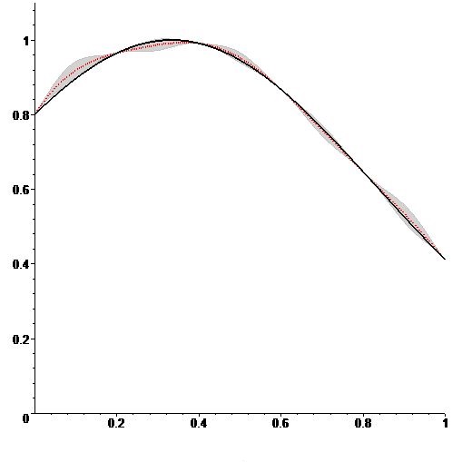
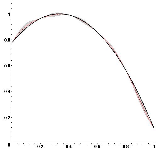
Figure 1: Kriging confidence regions for kernel approximation of $f_{1}$ (left) and $f_{2}$ (right): Gaussian kernel, $\lambda=15$, $N=6$.

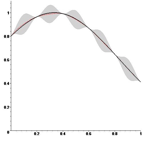
Figure 2: Kriging confidence regions for kernel approximation of $f_{1}$ (left) and $f_{2}$ (right): Cauchy kernel, $\lambda=20$, $N=6$.

The results for the Gaussian kernel $K(x,y)=\sigma^{2}\exp\{-15(x-y)^{2}\}$ are depicted on Figs. 1 and 3. The corresponding results for the Cauchy kernel $K(x,y)=\sigma^{2}/(1+20(x-y)^{2})$ can be found Figs. 2 and 4. It is clear from comparing left and right panels in Figs. 1–4 that kernel approximations for $f_{1}\in H(K)$ are significantly more accurate than for $f_{2}\notin H(K)$. The two chosen kernels (Gaussian with $\lambda=15$ and Cauchy with $\lambda=20$) look very similar but have different tail behaviour of the corresponding spectral density: the tail of the spectral density of the Cauchy kernel has a heavier tail. The confidence regions for the regression function constructed by the Cauchy kernel are rather wide and resemble the regions for the Matérn kernels with shape parameters 3/2 and 5/2 having similar correlation lengths. The confidence regions in the case of Gaussian kernel are much narrower (in fact, far too narrow) and the confidence regions for the kernels in (E.3) and (E.4) of Section 1.3 are even narrower; the spectral measures for these kernels have finite support.

In Figure 5 we plot the deviations and confidence regions for kernel approximation with Gaussian kernel $K(x,y)=\sigma^{2}\exp\{-2(x-y)^{2}\}$; the Gaussian kernel with $\lambda=2$ is perfectly suited for function $f_{1}$. A naive visual inspection of the two functions might suggest the Gaussian kernel should also work well for $f_{2}$ but, as we can observe from Figure 5 (right), it is not so for $f_{2}\notin H(K)$. The confidence region on Figure 5 (right) cannot be seen as the deviations $|\mu_{N}(x)-f_{2}(x)|$ are on average $10^{5}$ times larger than $3\widehat{\sigma^{2}_{N}}\,C_{N}(x,x)$.

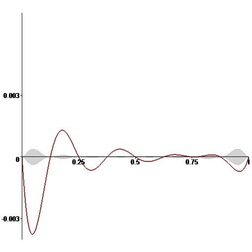
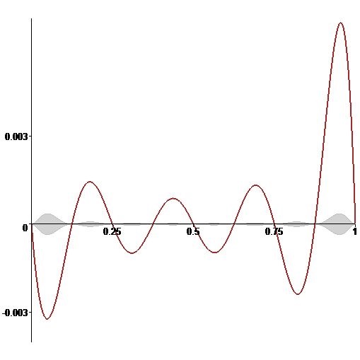
Figure 3: Deviation and confidence bounds in kernel approximation: Gaussian kernel, $\lambda=15$, $N=9;$ $f_{1}$ (left) and $f_{2}$ (right)

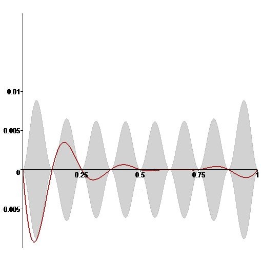
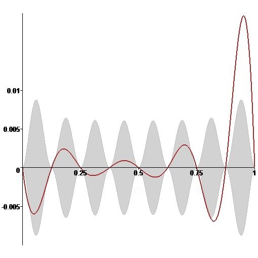
Figure 4: Deviation and confidence bounds in kernel approximation: Cauchy kernel, $\lambda=20$, $N=9;$ $f_{1}$ (left) and $f_{2}$ (right)

From the numerical studies partially illustrated in these figures we make the following conclusions concerning uncertainty quantification in GP regression models with infinitely differentiable translation-invariant kernels:

• if $f\notin H(K)$, then the kriging confidence regions for $f$ are always inaccurate;

• the heavier are the tails of the spectral measure of the kernel, the wider are the confidence regions;

• if the tail of the spectral measure of the kernel is light and the function $f$ does not belong to the respective RKHS, then the kernel approximation of $f$ appears to be rather inaccurate and the confidence regions seem to be missing $f$ almost entirely;

• if the function $f$ does not belong to the respective RKHS, then $\widehat{\sigma^{2}_{N}}\to\infty$ as $N\to\infty$, but this has little effect on the size of the confidence intervals, at least for small $N$;

• for kernels with light tails of the respective spectral measures, the kernel approximation is accurate and confidence regions are adequate only if the shape of $f$ precisely matches the shape of the kernel functions $K(x,\cdot)$, as in Figure 5 (left).

Acknowledgements This research was partially supported by the research grant DFG DE 502/27-1 of the German Research Foundation (DFG). The authors are grateful to Timo Karvonen (Alan Turing Institute) for intelligent discussions, spotting an essential typo and pointing out several important references. We would also like to thank both referees and especially the associate editor for their constructive and very valuable comments on earlier versions of this paper.

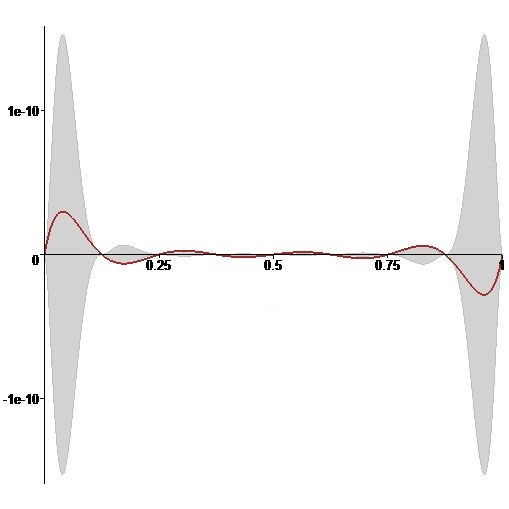
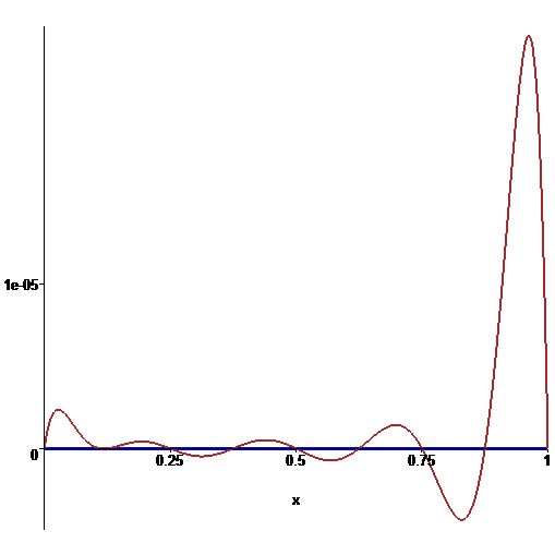
Figure 5: Deviation and confidence bounds in kernel approximation: Gaussian kernel, $\lambda=2$, $N=9;$ $f_{1}$ (left) and $f_{2}$ (right).

References

- Achieser, (1956) Achieser, N. I. (1956). Theory of Approximation. Frederick Ungar Publishing Co., N.Y.
- Akhiezer, (1965) Akhiezer, N. (1965). The Classical Moment Problem and Some Related Questions in Analysis. Oliver & Boyd.
- Archetti and Candelieri, (2019) Archetti, F. and Candelieri, A. (2019). Bayesian Optimization and Data Science. Springer.
- Berg et al., (2002) Berg, C., Chen, Y., and Ismail, M. E. (2002). Small eigenvalues of large Hankel matrices: The indeterminate case. Mathematica Scandinavica, 90:67–81.
- Berlinet and Thomas-Agnan, (2011) Berlinet, A. and Thomas-Agnan, C. (2011). Reproducing Kernel Hilbert Spaces in Probability and Statistics. Springer.
- Billingsley, (2008) Billingsley, P. (2008). Probability and Measure. John Wiley & Sons, forth edition.
- Bochner and Chandrasekharan, (1949) Bochner, S. and Chandrasekharan, K. (1949). Fourier Transforms. (AM-19). University Press, Princeton, N.J.
- Briol et al., (2019) Briol, F.-X., Oates, C., Girolami, M., Osborne, M., and Sejdinovic, D. (2019). Probabilistic integration: A role in statistical computation? Statistical Science, 34(1):1–22.
- Cambanis and Masry, (1983) Cambanis, S. and Masry, E. (1983). Sampling designs for the detection of signals in noise. IEEE Transactions on Information Theory, 29(1):83–104.
- Dette et al., (2019) Dette, H., Pepelyshev, A., and Zhigljavsky, A. (2019). The BLUE in continuous-time regression models with correlated errors. Annals of Statistics, 47(4):1928–1959.
- Dette and Studden, (1992) Dette, H. and Studden, W. (1992). On a new characterization of the classical orthogonal polynomials. Journal of Approximation Theory, 71(1):3–17.
- Dette and Studden, (1997) Dette, H. and Studden, W. (1997). The Theory of Canonical Moments with Applications in Statistics, Probability and Analysis. John Wiley & Sons.
- Hennig et al., (2015) Hennig, P., Osborne, M., and Girolami, M. (2015). Probabilistic numerics and uncertainty in computations. Proceedings of the Royal Society A: Mathematical, Physical and Engineering Sciences, 471(2179):20150142.
- Heyde, (1963) Heyde, C. (1963). Some remarks on the moment problem (i). The Quarterly Journal of Mathematics, 14(1):91–96.
- Kanagawa et al., (2018) Kanagawa, M., Hennig, P., Sejdinovic, D., and Sriperumbudur, B. (2018). Gaussian processes and kernel methods: A review on connections and equivalences. arxiv e-prints, art. arXiv preprint arXiv:1807.02582.
- Karvonen, (2021) Karvonen, T. (2021). On non-inclusion of certain functions in reproducing kernel Hilbert spaces. arXiv preprint arXiv:2102.10628.
- Karvonen et al., (2020) Karvonen, T., Wynne, G., Tronarp, F., Oates, C., and Särkkä, S. (2020). Maximum likelihood estimation and uncertainty quantification for Gaussian process approximation of deterministic functions. SIAM/ASA J. on Uncertainty Quantification, 8(3):926–958.
- Krantz and Parks, (2002) Krantz, S. and Parks, H. (2002). A Primer of Real Analytic Functions. Springer.
- Lau and Studden, (1988) Lau, T.-S. and Studden, W. (1988). On an extremal problem of Fejér. Journal of Approximation Theory, 53(2):184–194.
- Lee et al., (2016) Lee, K.-Y., Li, B., and Zhao, H. (2016). Variable selection via additive conditional independence. Journal of the Royal Statistical Society B, 78(5):1037–1055.
- Lin, (2017) Lin, G. D. (2017). Recent developments on the moment problem. Journal of Statistical Distributions and Applications, 4(1):1–17.
- Minh, (2010) Minh, H. Q. (2010). Some properties of Gaussian reproducing kernel Hilbert spaces and their implications for function approximation and learning theory. Constructive Approximation, 32(2):307–338.
- Parzen, (1961) Parzen, E. (1961). An approach to time series analysis. The Annals of Mathematical Statistics, 32(4):951–989.
- Paulsen and Raghupathi, (2016) Paulsen, V. and Raghupathi, M. (2016). An Introduction to the Theory of Reproducing Kernel Hilbert Spaces. Cambridge university press.
- Pronzato and Zhigljavsky, (2020) Pronzato, L. and Zhigljavsky, A. (2020). Bayesian quadrature, energy minimization, and space-filling design. SIAM/ASA Journal on Uncertainty Quantification, 8(3):959–1011.
- Rasmussen and Williams, (2006) Rasmussen, C. and Williams, C. (2006). Gaussian Processes for Machine Learning. MIT Press.
- Ritter, (2007) Ritter, K. (2007). Average-Case Analysis of Numerical Problems. Springer.
- Ritter et al., (1995) Ritter, K., Wasilkowski, G., and Woźniakowski, H. (1995). Multivariate integration and approximation for random fields satisfying Sacks-Ylvisaker conditions. The Annals of Applied Probability, 5(2):518–540.
- Scheuerer et al., (2013) Scheuerer, M., Schaback, R., and Schlather, M. (2013). Interpolation of spatial data–a stochastic or a deterministic problem? European Journal of Applied Mathematics, 24(04):601–629.
- Schmüdgen, (2017) Schmüdgen, K. (2017). The Moment Problem. Springer.
- Schulz et al., (2018) Schulz, E., Speekenbrink, M., and Krause, A. (2018). A tutorial on Gaussian process regression: Modelling, exploring, and exploiting functions. Journal of Mathematical Psychology, 85:1–16.
- Shohat and Tamarkin, (1943) Shohat, J. and Tamarkin, J. (1943). The Problem of Moments. American Math. Soc.
- Stein, (1999) Stein, M. L. (1999). Interpolation of Spatial Data: Some Theory for Kriging. Springer.
- Steinwart and Christmann, (2008) Steinwart, I. and Christmann, A. (2008). Support Vector Machines. Springer.
- Steinwart et al., (2006) Steinwart, I., Hush, D., and Scovel, C. (2006). An explicit description of the reproducing kernel Hilbert spaces of Gaussian RBF kernels. IEEE Trans. on Inform. Theory, 52(10):4635–4643.
- Stoyanov, (2013) Stoyanov, J. M. (2013). Counterexamples in Probability. Courier Corporation.
- Sun and Zhou, (2008) Sun, H.-W. and Zhou, D.-X. (2008). Reproducing kernel Hilbert spaces associated with analytic translation-invariant Mercer kernels. Journal of Fourier Analysis and Applications, 14(1):89–101.
- Wainwright, (2019) Wainwright, M. (2019). High-dimensional statistics: A non-asymptotic viewpoint. Cambridge University Press.
- Wendland, (2004) Wendland, H. (2004). Scattered Data Approximation. Cambridge university press.
- Xu and Stein, (2017) Xu, W. and Stein, M. L. (2017). Maximum likelihood estimation for a smooth Gaussian random field model. SIAM/ASA Journal on Uncertainty Quantification, 5(1):138–175.
- Yaglom, (1986) Yaglom, A. (1986). Correlation Theory of Stationary and Related Random Functions. Volume I: Basic Results. Springer.
- Zhigljavsky and Žilinskas, (2021) Zhigljavsky, A. and Žilinskas, A. (2021). Bayesian and High-Dimensional Global Optimization. Springer.