A Machine Learning Challenge for Prognostic Modelling in Head and Neck Cancer Using Multi-modal Data

Abstract

Accurate prognosis for an individual patient is a key component of precision oncology. Recent advances in machine learning have enabled the development of models using a wider range of data, including imaging. Radiomics aims to extract quantitative predictive and prognostic biomarkers from routine medical imaging, but evidence for computed tomography radiomics for prognosis remains inconclusive. We have conducted an institutional machine learning challenge to develop an accurate model for overall survival prediction in head and neck cancer using clinical data etxracted from electronic medical records and pre-treatment radiological images, as well as to evaluate the true added benefit of radiomics for head and neck cancer prognosis. Using a large, retrospective dataset of 2,552 patients and a rigorous evaluation framework, we compared 12 different submissions using imaging and clinical data, separately or in combination. The winning approach used non-linear, multitask learning on clinical data and tumour volume, achieving high prognostic accuracy for 2-year and lifetime survival prediction and outperforming models relying on clinical data only, engineered radiomics and deep learning. Combining all submissions in an ensemble model resulted in improved accuracy, with the highest gain from a image-based deep learning model. Our results show the potential of machine learning and simple, informative prognostic factors in combination with large datasets as a tool to guide personalized cancer care.

Introduction

The ability of computer algorithms to assist in clinical oncology tasks, such as patient prognosis, has been an area of active research since the 1970’s [1]. More recently, machine learning (ML) and artificial intelligence (AI) have emerged as a potential solution to process clinical data from multiple sources and aid diagnosis [2], prognosis [3] and course of treatment decisions [4], enabling a more precise approach to clinical management taking individual patient characteristics into account [5]. The need for more personalized care is particularly evident in head and neck cancer (HNC), which exhibits significant heterogeneity in clinical presentation, tumour biology and outcomes [6, 7], making it difficult to select the optimal management strategy for each patient. Hence, there is a current need for better predictive and prognostic tools to guide clinical decision making [8, 9].

One potential source of novel prognostic information is the imaging data collected as part of standard care. Imaging data has the potential to increase the scope of relevant prognostic factors in a non-invasive manner as compared to genomics or pathology, while high volume and intrinsic complexity render it an excellent use case for machine learning. Radiomics is an umbrella term for the emerging field of research aiming to develop new non-invasive quantitative prognostic and predictive imaging biomarkers using both hand-engineered [10] and deep learning techniques [11]. Retrospective radiomics studies have been performed in a variety of imaging modalities and cancer types for a range of endpoints.

In HNC, radiomics has been used [12] to predict patient outcomes [13, 14], treatment response [15, 16], toxicity [17, 18], and discover associations between imaging and genomic markers [19, 20]. In a recent MICCAI Grand Challenge, teams from several different institutions competed to develop the best ML approach to predict human papillomavirus (HPV) status using a public HNC dataset [21].

Despite the large number of promising retrospective studies, the adoption of prognostic models utilizing radiomics into clinical workflows is limited [22, 23]. There has also been growing concern regarding the lack of transparency and reproducibility in ML research, which are crucial to enabling widespread adoption of these tools [24, 25]. Although significant progress has been made in certain areas (e.g. ensuring consistency between different engineered feature toolkits [26]) many studies do not make the code or data used for model development publicly available, and do not report key details of data processing, model training and validation, making it challenging to reproduce, validate and build upon their findings [22, 27]. Additionally, the lack of large, standardized benchmark datasets makes comparing different approaches challenging, with many publications relying on small, private datasets. Furthermore, there is mounting evidence that the current methods of image quantification based on engineered features are largely correlated and redundant to accepted clinical biomarkers [28, 13, 29]. Approaches based on deep learning have been steadily gaining popularity, but it is still unclear whether they share these pitfalls and truly improve prognostic performance.

We have conducted an institutional ML challenge to develop a prognostic model for HNC using routine CT imaging and data from electronic medical records (EMR), engaging a group of participants from diverse academic background and knowledge. In this manuscript we will describe in detail the challenge framework, prognostic model submissions and final results. A key strength of our approach is the rigorous evaluation framework, enabling rigorous comparison of multiple ML approaches using EMR data as well as engineered and deep radiomics in a large dataset of 2,552 HNC patients. We make the dataset and the code used to develop and evaluate the challenge submissions publicly available for the benefit of the broader community.

Results

Dataset

For the purpose of the challenge, we collected a combined EMR (i.e. clinical, demographic and interventional data) and imaging dataset of 2,552 HNC patients treated with radiation therapy or chemoradiation at Princess Margaret Cancer Centre (PM). The dataset was divided into a training set (70%) and an independent test set (30%). In order to simulate a prospective validation we chose to split the data by date of diagnosis at a pre-defined time point. We made pre-treatment contrast-enhanced CT images and binary masks of primary gross tumour volumes (GTV) available to the participants. We also released a set of variables extracted from EMR, including demographic (age at diagnosis, sex), clinical (T, N and overall stage, disease site, performance status and HPV infection status) and treatment-related (radiation dose in Gy, use of chemotherapy) characteristics (fig. 1). Additionally, outcome data (time to death or censoring, event indicator) was available for training data only.

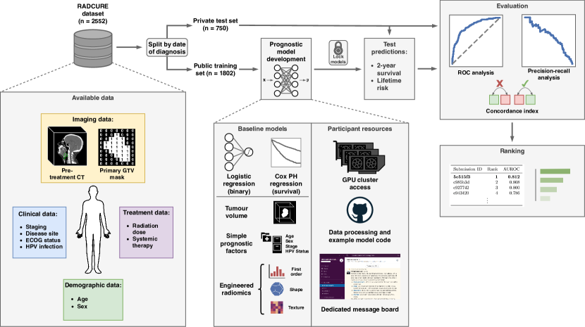
Figure 1: Overview of challenge and dataset. EMR and imaging data from a large cohort of HNC patients were available to the participants. The training set, consisting of patients diagnosed before a pre-specified date was released together with the ground-truth outcome information and used for prognostic model development. The test set was kept private and only made available (without outcome data) after the development phase was completed. The participants submitted their test set predictions, which were evaluated by the organizers. We provided the participants with a rich set of resources, including access to a computing cluster with general purpose graphics processing units (GPUs), a Github repository containing the code used for data processing and submission evaluation together with example model implementation, as well as a dedicated Slack workspace used for announcements, communication between participants and organizers and technical support. We also developed a set of simple but strong baseline models to serve as benchmark for comparison as well as a reference point for the participants during the development stage.

Challenge description and evaluation criteria

The challenge organization process is summarized in fig. 1. The challenge was open to anyone within the University Health Network. Study design and competition rules were fully specified and agreed upon by all participants prior to the start. All participants had access to the training data with ground-truth outcome labels, while the test set was held out for final evaluation. The primary objective was to predict 2-year overall survival (OS), with the secondary goals of predicting a patient’s lifetime risk of death and full survival curve. We chose the binary endpoint as it is commonly used in the literature and readily amenable to many standard ML methods. The primary evaluation metric for the binary endpoint, which was used to rank the submissions, was the area under receiver operating characteristic curve (AUROC). We also used average precision (AP) as a secondary performance measure to break any submission ties, due to its higher sensitivity to class imbalance [30]. Submission of lifetime risk and survival curve predictions was optional, and they were scored using the concordance ($C$) index [31]. Importantly, the participants were blinded to test set outcomes and only submitted predictions to be evaluated by the organizers. We additionally created a set of benchmark models for comparison (see Methods). We did not enforce any particular model type, image processing or input data (provided it was part of the official training set), although we did encourage participants to submit predictions based on EMR features, images, and combined data separately (if they chose to use all of the data modalities).

Overview of submissions

We received 12 submissions in total, which can be broadly classified as using EMR factors only, imaging only, or combining all data sources. In addition to the required 2-year event probabilities, 10 submissions included lifetime risk predictions and 7 included the full predicted survival curves. All submitted models performed significantly better than random on all performance measures ($p<.0001$ by permutation test). The top submission performed significantly better in terms of AUROC than every other submission ($\mathrm{FDR}<.05$), except the second-best ($\mathrm{FDR}>.05$ Most participants who used the imaging data relied on convolutional neural networks (convnets) to automatically learn predictive representations; only 2 combined and 1 radiomics-only submission used handcrafted features. Of the submitted convnets, 2 out of 3 relied on three-dimensional (3D) convolution operations. Although all EMR-only approaches used the same input data, there was significant variation in the kind of model used (linear and nonlinear, binary classifiers, proportional hazards and multi-task models, fig. 2(a)). The combined submissions used EMR data together with either tumour volume ($n=2$), engineered radiomics ($n=1$) or deep learning ($n=3$). A brief overview of all submissions is presented in table LABEL:tab:results_summary; for detailed descriptions, see Supplementary Material.

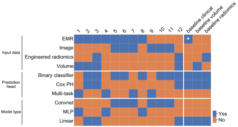
(a)

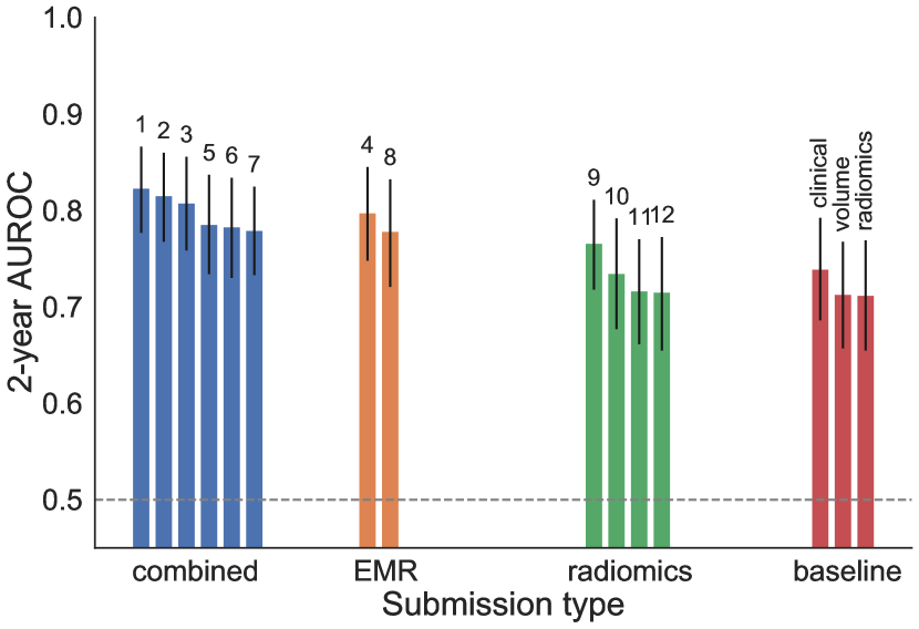
(b)

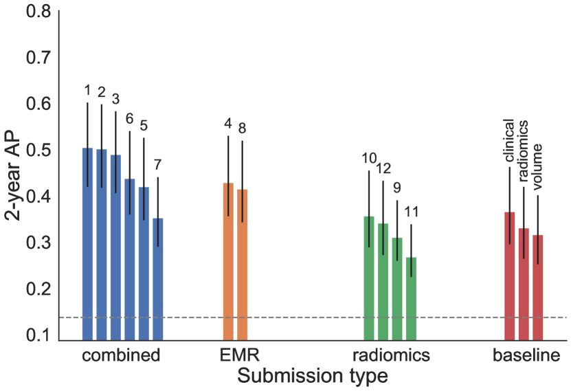
(c)

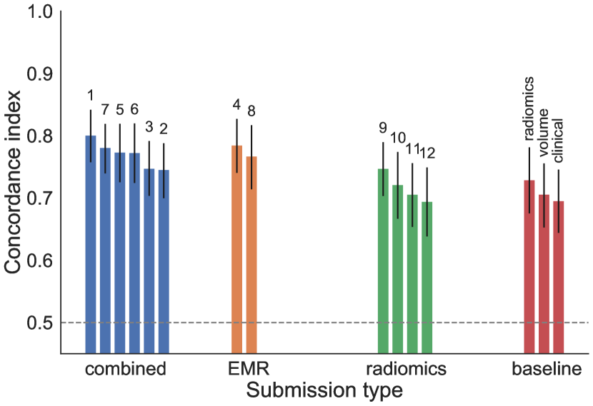
(d)

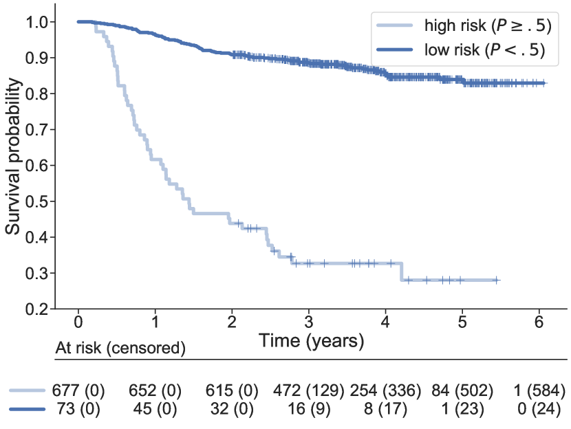
(e)

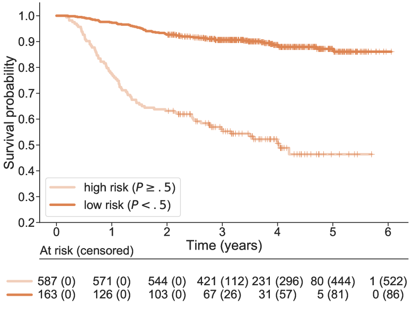
(f)

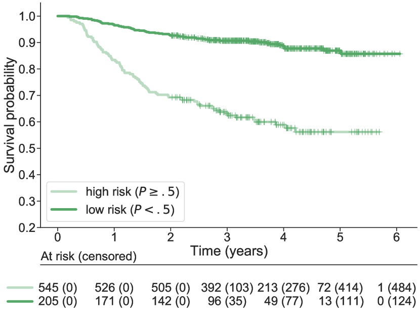
(g)

Figure 2: Challenge results. (a) Overview of submission characteristics. The characteristics are grouped into input data, prediction head (i.e. how were the survival predictions made) and model type (whether the model involved any nonlinearities and/or convolutions). PH: proportional hazards, MLP: multilayer perceptron, *: age, sex, stage, HPV status. (b,c,d) Performance of all challenge submissions and benchmark models in terms of 2-year AUROC, 2-year average precision and concordance index of the lifetime risk respectively. The results are ranked by AUROC (numbers above bars indicate the overall rank of each submission). Error bars represent 95% confidence intervals computed using 10,000 stratified bootstrap replicates. Dashed grey lines indicate random guessing performance (.5 for AUROC and $C$-index, .14 for AP). (e,f,g) show the Kaplan-Meier survival estimates in low and high risk groups identified by the best performing model in each challenge category (combined, EMR only and radiomics) respectively. Test set patient were stratified into 2 groups based on the predicted 2-year event probability at .5 threshold. In each case, there were significant differences in survival between the predicted risk groups (hazard ratio 8.64, 5.96 and 4.50 respectively, $p<10^{-18}$ for all).

Table 1: Summary of challenge submissions and performance metrics.

Rank	Description	AUROC	AP	$C$-index
1	Deep multi-task logistic regression using EMR features and tumour volume.	0.823 [0.777–0.866]	0.505 [0.420–0.602]	0.801 [0.757–0.842]
2	Fuzzy logistic regression (binary) and Cox proportional hazards model (risk prediction) using EMR features and tumour volume.	0.816 [0.767–0.860]	0.502 [0.418–0.598]	0.746 [0.700–0.788]
3	Fuzzy logistic regression (binary) or Cox proportional hazards model (risk prediction) using EMR features and engineered radiomic features.	0.808 [0.758–0.856]	0.490 [0.406–0.583]	0.748 [0.703–0.792]
4	Multi-task logistic regression using EMR features.	0.798 [0.748–0.845]	0.429 [0.356–0.530]	0.785 [0.740–0.827]
5	3D convnet using cropped image patch around the tumour with EMR features concatenated before binary classification layer.	0.786 [0.734–0.837]	0.420 [0.347–0.525]	0.774 [0.725–0.819]
6	2D convnet using largest GTV image and contour slices with EMR features concatenated after additional non-linear encoding before binary classification layer.	0.783 [0.730–0.834]	0.438 [0.360–0.540]	0.773 [0.724–0.820]
7	3D DenseNet using cropped image patch around the tumour with EMR features concatenated before multi-task prediction layer.	0.780 [0.733–0.824]	0.353 [0.290–0.440]	0.781 [0.740–0.819]
8	Multi-layer perceptron (MLP) with SELU activation and binary output layer using EMR features.	0.779 [0.721–0.832]	0.415 [0.343–0.519]	0.768 [0.714–0.817]
9	Two-stream 3D DenseNet with multi-task prediction layer using cropped patch around the tumour and additional downsampled context patch.	0.766 [0.718–0.811]	0.311 [0.260–0.391]	0.748 [0.703–0.790]
10	2D convnet using largest GTV image and contour slices and binary output layer.	0.735 [0.677–0.792]	0.357 [0.289–0.455]	0.722 [0.667–0.774]
11	3D convnet using cropped image patch around the tumour and binary output layer.	0.717 [0.661–0.770]	0.268 [0.225–0.339]	0.706 [0.653–0.756]
12	Fuzzy logistic regression (binary) and Cox proportional hazards model (risk prediction) using engineered radiomic features.	0.716 [0.655–0.772]	0.341 [0.272–0.433]	0.695 [0.638–0.749]

Deep learning using imaging only achieves good performance and outperforms engineered radiomics

Among the radiomics-only models, deep learning-based approaches performed better than hand-engineered features. In particular, nearly all deep learning models (except one) outperformed baseline-radiomics and challenge submissions (submission 12, fig. 2) in the binary prediction task (the smaller differences in $C$-index can be explained by the fact that most of the deep models were designed for binary classification only, and we used their binary predictions as a proxy for lifetime risk scores). We note that it is difficult to draw definitive conclusions due to the large number of radiomics toolkits and the wealth of feature types and configuration options they offer [26]. Nevertheless, the results show that a carefully-tuned DL model can learn features with superior discriminative power given a sufficiently large dataset.

The convnet-based models show varying levels of performance, most likely due to differences in architectures and prior image processing. Notably, the best 3D architecture (submission 9) achieves superior performance to the 2D VGGNet (number 10). It incorporates several innovative features, including dense connectivity [32, 33], two-stream architecture with a downsampled context window around the tumour and a dedicated survival prediction head (detailed description in Supplementary Material).

EMR features show better prognostic value than deep learning, even in combination

While radiomics can be a strong predictor of survival on its own, the small performance gap between EMR and combined models using deep radiomics (submissions 4, 6, 7) in most cases suggests the models do not learn complementary image representations and that the performance is driven primarily by the EMR features (fig. 2). Although one combined submission using engineered features (number 3) achieved good performance, it performed worse than the exact same model using EMR features and volume only (number 2), indicating that adding radiomic features reduces performance, and the engineered features were not strong predictors on their own. Moreover, none of the radiomics-only models performed better than any of the EMR-only submissions (although one convnet did outperform baseline-clinical). A possible explanation is suboptimal model design that fails to exploit the complementarity between the data sources. All of the deep learning solutions incorporated EMR features in a rather ad hoc fashion by concatenating them with the image representation vector and passing them to the final classification layer. While this approach is widely used, it is not clear that it is optimal in this context. More sophisticated methods of incorporating additional patient-level information, such as e.g. joint latent spaces [34] should be explored in future research.

Impact of volume dependence on model performance

Recent literature has demonstrated that many radiomic signatures show strong dependence on tumour volume [28, 29], which is a simple image-derived feature and a known prognostic factor in HNC [35]. We evaluated the correlation of all binary predictions with volume using Spearman rank correlation (fig. 3). Both the baseline radiomics model and the submission using handcrafted features show high correlation (Spearman $\rho=.79$ and $\rho=.85$, respectively), suggesting that their predictions are driven primarily by volume dependency. The predictions of two out of three convnets also show some volume correlation, albeit smaller than engineered features ($\rho>.5$). Interestingly, predictions of the best radiomics-only model (submission 9) show only weak correlation with volume ($\rho=.22$) and are more discriminative than volume alone ($\mathrm{AUROC}=.77$), suggesting that it might be possible to learn volume-independent image-based predictors.

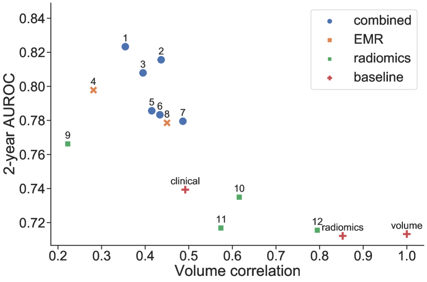
(a)

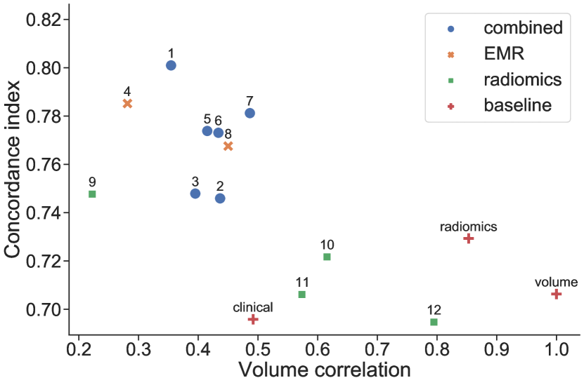
(b)

Figure 3: Volume dependence of predictions. Spearman rank correlation of the predictions of each submission with tumour volume against performance in terms of (a) AUROC and (b) $C$-index, respectively. The top submissions fall into an optimal region of low (but non-zero) volume correlation and high performance. Note that while submissions 1 and 2 used tumour volume as one of the input variables, their predictions correlate with volume only moderately ($\rho<.5$), indicating they are able to exploit additional information present in the EMR features. Higher correlation leads to decreased performance as the predictions are increasingly driven by volume only. Most radiomics-only submission fall in the high correlation region ($\rho\geq.5$), although deep learning predictions correlate at notably lower level than engineered features. Interestingly, the best radiomics submission (number 9) achieves the lowest volume correlation, suggesting that it might be using volume-independent imaging characteristics.

Winning Submission: Multi-task learning with simple image features and EMR data

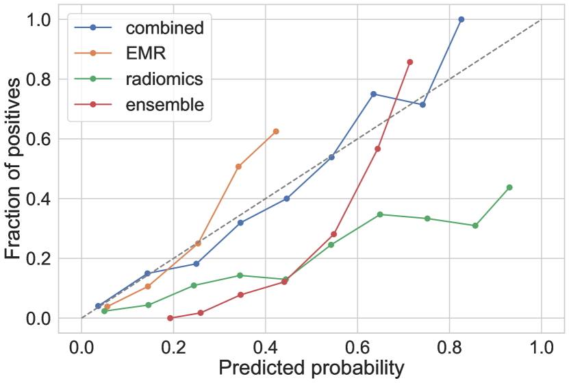
Figure S2: Calibration of predicted 2-year event probabilities for the best performing model in each category and the ensemble of all models.

The winning submission (number 1) combined EMR data with a simple image-derived measure, and used a ML model tailored to survival prediction; a schematic overview of the submission is shown in fig. 4. The approach is based on multi-task logistic regression (MTLR), first proposed by Yu et al [36]. In contrast with other approaches, which focused on the binary endpoint only, MTLR is able to exploit time-to-event information by fitting a sequence of dependent logistic regression models to each interval on a discretized time axis, effectively learning to predict a complete survival curve for each patient in multi-task fashion. By making no restrictive assumptions about the form of the survival function, the model is able to learn flexible relations between covariates and event probability that are potentially time-varying and non-proportional. We note that many prognostic models in clinical and radiomics literature use proportional hazards (PH) models [37, 38]; however, this ignores the potential time-varying effect of features which MTLR is able to learn. Notably, when compared to the second-best submission (which relies on a PH model) it achieves superior performance for lifetime risk prediction ($C=.801$ vs $.746$). The added flexibility and information-sharing capacity of multi-tasking also enables MTLR to outperform other submissions on the binary task ($\mathrm{AUROC}=.823$, $\mathrm{AP}=.505$), even though it is not explicitly trained to maximize predictive performance at 2 years; the predicted probabilities are also better calibrated (Supplementary Fig. S2). The winning approach relies on high-level EMR features which are widely-used, easy to interpret and show strong univariate association with survival (see Supplementary Material). The participant incorporated non-linear interactions by passing the features through a single-layer neural network with exponential linear unit (ELU) activation [39, 40], which resulted in better performance in the development stage. The only image-derived feature used is primary tumour volume, a known prognostic factor in HNC. Using EMR features only, led to a decrease in performance ($\mathrm{AUROC}=.798$, $\mathrm{AP}=.429$), as did replacing tumour volume with deep image representations learned by a 3D convnet ($\mathrm{AUROC}=.766$, fig. 4(b)).

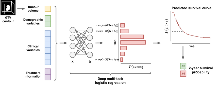
(a)

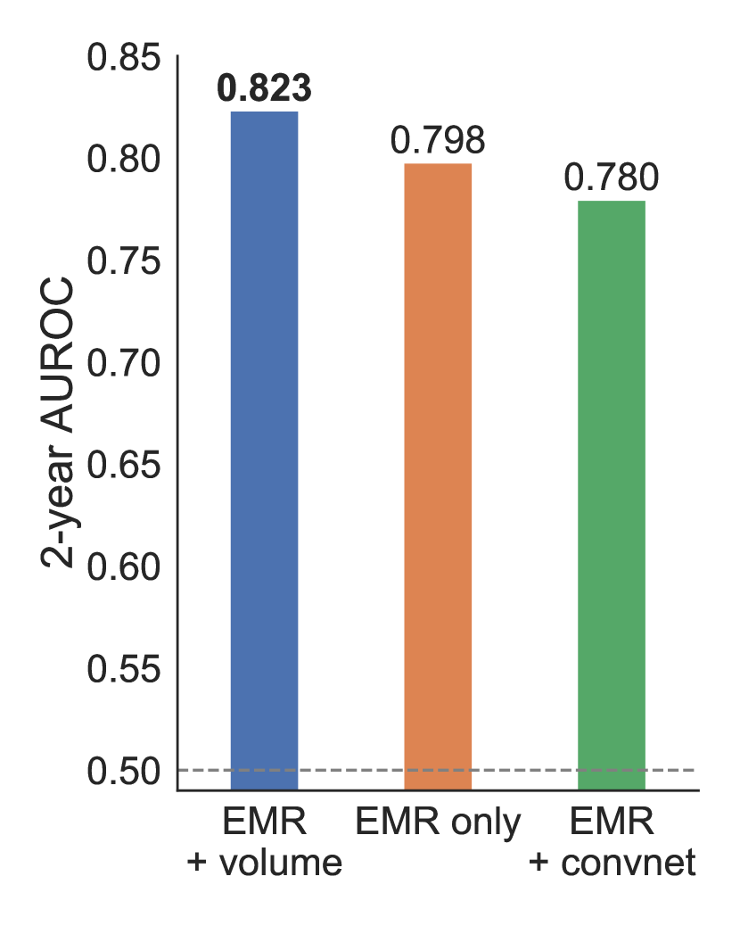
(b)

Figure 4: Winning submission. (a) Overview of Deep MTLR. The model combines EMR features with tumour volume using a neural network and learns to jointly predict the probability of death at all intervals on the discretized time axis, allowing it to achieve good performance in both the binarized and lifetime risk prediction tasks. A predicted survival curve can be constructed for each individual to determine the survival probability at any timepoint. (b) Importance of combined input data for performance on the binary endpoint. Training the deep MTLR on EMR features only led to notably worse performance. Furthermore, using a deep convolutional neural network in place of tumour volume did not improve the 2-year AUROC.

Ensemble of all models achieves improved performance, with largest gain from a deep learning model

Ensembling, i.e., combining predictions of multiple independent models, is known to yield superior performance to the individual predictors, as their errors tend to cancel out while correct predictions are reinforced [41]. We created an ensemble model from all submissions by averaging the submitted predictions. In the case of missing survival endpoint predictions, we used the 2-year survival probability as a proxy for overall risk to compute the $C$-index. The ensemble model achieves better performance in both 2-year and lifetime risk prediction ($\mathrm{AUROC}=.825$, $\mathrm{AP}=.495$,  $C=.808$) than any of the individual submissions (fig. 5). To investigate the risk stratification capacity, we split the test patients into 2 groups based on the ensemble predictions at .5 threshold. The ensemble approach was able to stratify the patients into low and high-risk groups with significantly different survival rates (hazard ratio 7.04, $p<10^{-27}$, fig. 5(c)) and placed nearly 40% of cancer-specific deaths in the top risk decile. Moreover, the predictions remained significantly discriminative even when adjusted for disease site ($p<10^{-32}$). It is, to our knowledge, the best published prognostic model for overall survival in HNC using EMR and imaging data. We examined the individual contributions to the ensemble performance by creating partial ensembles of progressively lower-ranking submissions (fig. 5(d)). Interestingly, adding the best radiomics submission (number 9) seems to provide the greatest performance improvement. Its predictions shows low correlation with volume and only moderate correlation with the winning model’s predictions, suggesting it might be learning prognostic signal distinct from volume and EMR characteristics.

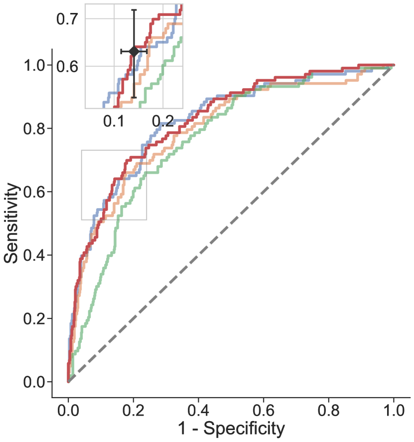
(a)

(b)

(c)

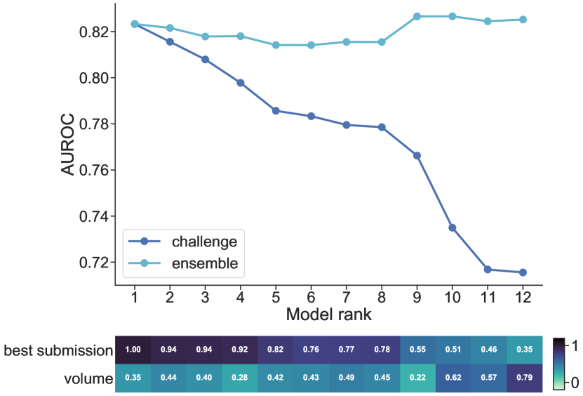
(d)

(e)

kind	AUROC	AP	C-index
ensemble	0.825 [0.781–0.866]	0.495 [0.414–0.591]	0.808 [0.770–0.843]
combined	0.823 [0.777–0.866]	0.505 [0.420–0.602]	0.801 [0.757–0.842]
EMR	0.798 [0.748–0.845]	0.429 [0.356–0.530]	0.785 [0.740–0.827]
radiomics	0.766 [0.718–0.811]	0.357 [0.289–0.455]	0.748 [0.703–0.790]
baseline-clinical	0.739 [0.686–0.792]	0.366 [0.295–0.463]	0.696 [0.644–0.746]
baseline-volume	0.713 [0.657–0.767]	0.317 [0.252–0.401]	0.706 [0.653–0.756]
baseline-radiomics	0.712 [0.655–0.769]	0.331 [0.264–0.420]	0.729 [0.675–0.781]

Figure 5: Performance of the ensemble approach. a) ROC and b) precision-recall curves of the ensemble model and the best challenge submission in each category. Sensitivity and (1 - specificity) at the operating point chosen for risk stratification are indicated with bootstrap 95% confidence intervals. c) Kaplan-Meier survival curves of the low (green) and high risk (red) subgroups identified by the ensemble model. d) Contribution of individual submissions to ensemble performance. Starting from the highest-ranking submissions, subset ensembles were created from progressively lower-ranking models. Rank=12 corresponds to the full ensemble AUROC. The individual AUROC values are shown for reference. The heatmap shows the correlation of predictions of each individual model with best submission predictions (top) and tumour volume (bottom). e) Performance comparison between the ensemble, best submission from each category and baseline models.

Discussion

We presented the results of a machine learning challenge for HNC survival prediction. The key strength of the proposed framework, inspired by the NCI DREAM challenges for drug activity prediction [42], is the possibility of rigorous and reproducible evaluation of multiple ML approaches in a large, multi-modal dataset [43]. Additionally, the different participants’ academic backgrounds and computational approaches used resulted in a diverse collection of models and made it possible to build a ’wisdom of the crowds’ ensemble model with improved performance.

The best individual approach achieved strong performance on both 2-year and lifetime risk prediction using a multi-task survival modelling framework. This demonstrates the benefit of using a flexible approach designed specifically for the task of survival prediction. Additionally, because the approach relies on widely used and easy-to-interpret features (e.g. tumour stage, volume), it is attractive from a clinical standpoint as a risk stratification and monitoring tool. Our best ensemble model combined the strengths of all submissions to establish, to our knowledge, a new state-of-the-art result for HNC survival prediction. The model predictions are highly significant, even when adjusted for disease site, demonstrating the potential of learning from large cross-sectional datasets, as opposed to highly curated patient subsets (which has been the dominant paradigm thus far).

The utility of radiomics in HNC survival prediction has been investigated in recent studies [15, 16, 13]. We have identified several strong radiomics predictors; however, the best performing individual submission used EMR features, with primary tumour volume as the only image-derived feature. Our conclusions match those of Ger et al. [13], who did not find significant improvement in prognostic performance of handcrafted CT and PET imaging features in HNC compared to volume alone and of Vallières et al. [15], whose best performing model for overall survival also combined EMR features and volume. We further showed that although deep learning-based imaging models generally outperformed approaches based on handcrafted features, none proved superior to the combined EMR-volume model, even when combined with EMR data. Deep learning methods achieve excellent performance in many image processing tasks [44], however, current approaches require substantial amounts of training data.

While our dataset is the largest publicly-available HCN imaging collections, it is still relatively small compared to natural image datasets used in ML research, which often contain millions of samples [45]. Although such large sample sizes might be unachievable in this particular setting, better data collection and sharing practices can help build more useful databases (the UK Biobank [46] or the Cancer Genome Atlas [47] are excellent examples). This is especially important in diseases with low event rates, where a substantial number of patients might be needed to capture the variation in phenotype and outcomes. The inferior performance of radiomic models can also be attributed to suboptimal imaging data. While the possibility to easily extract retrospective patient cohorts makes routine clinical images attractive for radiomics research, they are often acquired for purposes entirely orthogonal to new biomarker discovery. CT images in particular might not accurately reflect the biological tumour characteristics due to insufficient resolution, sensitivity to acquisition parameters and noise [48, 49], as well as the source of image contrast, which is essentially electron density of the tissue which demonstrates little texture at current image scales. This highlights the broader need of greater collaboration between ML researchers, clinicians and physicists, also in data selection and experiment design — with reciprocal feedback [50, 51].

Our study has several potential limitations. Participation was restricted to one institution, which limited the number of submissions we received. Additionally, the hand-engineered radiomics submissions relied on one radiomics toolkit (PyRadiomics) and other widely-used toolkits make use of potentially different feature sets and definitions; however, thanks to recent efforts in image biomarker standardization, the features have been shown to be largely consistent between the major implementations [26]. Additionally, our dataset was collected within one hospital only. Assessing generalizability of the best performing models to other institutions and patient populations is important for future clinical implementation. This is particularly relevant for radiomics models as domain shift due to differences in scanning equipment and protocols could negatively affect generalization and we are currently working on validating the best performing models using multi-institutional data. It is likely that more sophisticated ensembling methods (e.g. Bayesian model averaging [41] or stacking [52]) could achieve even better performance by weighing the models according to their strengths. We leave this exploration for future work.

In the future, we would like to open the challenge to a larger number of participants, which would further enhance the diversity of approaches and help us validate our conclusions. We are also working on collecting additional outcome information, including recurrence, distant metastasis and treatment toxicity, which would provide a richer set of prediction targets and might be more relevant from a clinical standpoint. The importance of ML and AI as tools of precision medicine will continue to grow. However, it is only through transparent and reproducible research that integrates diverse knowledge that we can begin to realize the full potential of these methods and permit integration into clinical practice.

Methods

Dataset

We collected a retrospective dataset of 2552 HNC patients treated with radiotherapy or chemoradiation at PM Cancer Centre between 2005 and 2017 (Supplementary table S1), which we split into training and test subsets by date of diagnosis (2005-2015 and 2016-2018 for training and independent test set, respectively). The study was approved by the institutional Research Ethics Board (REB #17-5871). The inclusion criteria were: 1) availability of planning CT image and target contours; 2) at least 2 years follow-up (or death before that time); and 3) no distant metastases at diagnosis and no prior surgery. Primary gross tumour volumes (GTV) were delineated by radiation oncologists as part of routine treatment planning. For each patient we exported the CT image and primary GTV binary mask in NRRD format. We also extracted the follow-up information (current as of April 2020). The dataset was split into training ($n=1802$) and test ($n=750$) subsets according to the date of diagnosis (Supplementary fig. S1).

Baseline models

To provide baselines for comparison and a reference point for the participants, we created three benchmark models using: 1) standard prognostic factors used in the clinic (age, sex, T/N stage and HPV status) (baseline-clinical); 2) primary tumour volume only (baseline-volume); 3) handcrafted imaging features (baseline-radiomics). All categorical variables were one-hot encoded and missing data was handled by creating additional category representing missing value (e.g. ’Not tested’ for HPV status). For the baseline-radiomics model, we extracted all available first order, shape and textural features from the original image and all available filters (1316 features in total) using the PyRadiomics package (version 2.2.0) [53] and performed feature selection using maximum relevance-minimum redundancy (MRMR) method [54]. The number of selected features and model hyperparameters ($l_{2}$ regularization strength) were tuned using grid search with 5-fold cross validation. All models, were built using logistic regression for the binary endpoint and a proportional hazards model for the survival endpoint.

Participant resources

All participants had access to a shared Github repository containing the code used for data processing, as well as implementations of the baseline models and example modelling pipelines, facilitating rapid development process. A dedicated Slack workspace was used for announcements, communication with organizers and between participants and to share useful learning resources. We hosted the dataset on an institutional high-performance computing (HPC) cluster with multicore CPUs and general-purpose graphics processing units (GPUs) which were available for model training.

Tasks and performance metrics

The main objective of the challenge was to predict binarized 2-year overall survival (OS), with the supplementary task of predicting lifetime risk of death and full survival curves (in 1-month intervals from 0 to 23 months). To evaluate and compare model performance on the 2-year binarized survival prediction task, we used area under the ROC curve (AUROC), which is a ranking metric computed over all possible decision thresholds. We additionally computed the area under precision-recall curve, also referred to as average precision (AP), using the formula:

$$\mathrm{AP}=\sum_{n}(R_{n}-R_{n-1})P_{n},$$

where $R_{n}$ and $p_{n}$ are the precision and recall at a given threshold, respectively. While AUROC is insensitive to class balance, AP considers the positive class only, which can reveal pathologies under high class imbalance [55]. Additionally, both metrics consider all possible operating points, which removes the need to choose a particular decision threshold (which can vary depending on the downstream clinical task). Since the dataset did not include patients with follow-up time less than 2 years, we did not correct the binary metrics for censoring bias.

For the lifetime risk prediction task, we used concordance index, defined as:

$$C=\frac{\sum_{i\text{ uncensored}}\sum_{t_{j}>t_{i}}\mathbf{1}\{r_{i}>r_{j}\}+\frac{1}{2}\mathbf{1}\{r_{i}=r_{j}\}}{\sum_{i\text{ uncensored}}\mathbf{1}\{t_{j}>t_{i}\}},$$

where $t_{i}$ is the time until death or censoring for patient $i$, $r_{i}$ is the predicted risk score for patient $i$ and $\mathbf{1}\{\}$ is the indicator function. The agreement between the performance measures was good (Pearson $r=.88$ between AUROC and AP, $r=.82$ between AUROC and $C$-index). We compared the AUROC achieved by the best submission to the other submissions using one-sided $t$-test and corrected for multiple comparisons by controlling the false discovery rate (FDR) at .05 level.

Research reproducibility

The code used to prepare the data, train the baseline models, evaluate the challenge submissions and analyze the results is available on Github at https://github.com/bhklab/uhn-radcure-challenge. We also share the model code for all the challenge submissions with the participants’ permission in the same repository. Furthermore, we are planning to make the complete dataset, including anonymized images, contours and EMR data available on the Cancer Imaging Archive.

Supplementary material

Data curation and preprocessing

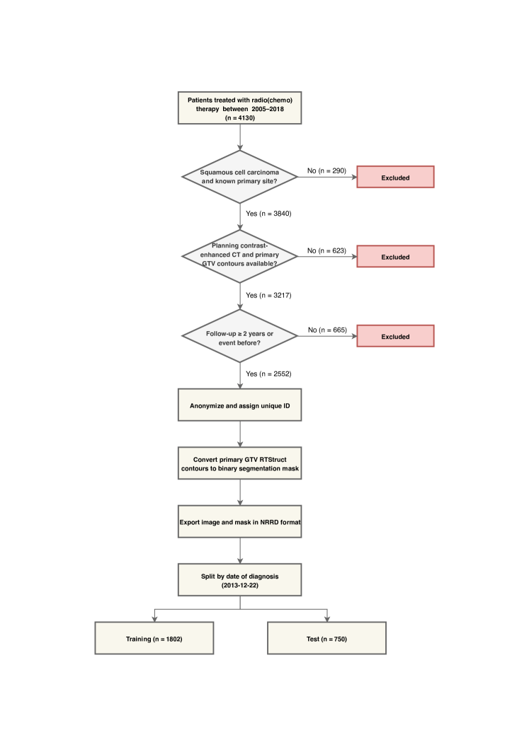
Figure S1: Patient selection and data curation process.

Patient characteristics

	Training	Test
# of patients	1802	750
Outcome
Alive/Censored	1065 (59%)	609 (81%)
Dead	737 (41%)	141 (19%)
Dead before 2 years	323 (18%)	103 (14%)
Sex
Male	1424 (79%)	615 (82%)
Female	378 (21%)	135 (18%)
Disease Site
Oropharynx	777 (43%)	399 (53%)
Larynx	555 (31%)	172 (23%)
Nasopharynx	220 (12%)	101 (13%)
Hypopharynx	115 (6.4%)	28 (3.7%)
Lip / Oral Cavity	72 (4.0%)	10 (1.3%)
Nasal Cavity	31 (1.7%)	20 (2.7%)
Paranasal Sinus	16 (0.9%)	10 (1.3%)
Esophagus	14 (0.8%)	8 (1.1%)
Salivary Glands	2 (0.1%)	2 (0.3%)
T stage
1/2	919 (51%)	405 (54%)
3/4	855 (47%)	336 (45%)
Not available	28 (2%)	9 (1%)
N stage
0	688 (38%)	226 (30%)
1	170 (9%)	90 (12%)
2	835 (46%)	395 (53%)
3	108 (6%)	39 (5%)
Not available	1 (<1%)	0 (0%)
AJCC stage
I/II	455 (25%)	158 (21%)
III/IV	1318 (73%)	581 (77%)
Not available	29 (2%)	11 (1%)
HPV status
Positive	513 (28%)	327 (44%)
Negative	269 (15%)	168 (22%)
Not tested	1020 (57%)	255 (34%)
Chemotherapy
Yes	725 (40%)	361 (48%)
No	1077 (60%)	389 (52%)
ECOG performance status
0	1120 (62%)	436 (58%)
1	489 (27%)	290 (39%)
2	145 (8%)	20 (3%)
>2	34 (2%)	4 (1%)
Not available	14 (1%)	0 (0%)

Table S1: Patient characteristics in the training and test sets.

Imaging protocols

Parameter	Median [range]
Slice thickness	2 [2–2.5]
kVp	120 [120–120]
Tube current [mAs]	300 [121–540]
Pixel spacing [mm]	(.976, .976) [(.702, .702)–(1.17, 1.17)]

Table S1: CT imaging parameters used in the study. Images were acquired using either of: Toshiba Aquilion One ($n=1653$), GE Discovery ST ($n=643$), GE LightSpeed Plus ($n=130$), Philips Brilliance Big Bore ($n=96$) or GE Discovery 610 ($n=30$).

*Detailed descriptions of submissions

Submission 1

Multi-task logistic regression (MTLR) uses a sequence of dependent regressors to predict the probability of event occuring at multiple discrete timepoints in a multi-task fashion [36]. The model is trained by minimizing the MTLR log-likelihood:

$$L(\boldsymbol{\Theta},D) =\sum_{j=1}^{N-N_{c}-1}\sum_{k=1}^{K-1}(\boldsymbol{\theta}_{k}^{T}\mathbf{\phi(x)}^{(j)}+b_{k})y_{k}^{(j)}$$ (Uncensored)

$$+\sum_{j=N-N_{c}}^{N}\log(\sum_{i=1}^{K-1}\mathbf{1}\{t_{i}\geq T_{c}^{(j)}\}\exp(\sum_{k=i}^{K-1}((\boldsymbol{\theta}_{k}^{T}\mathbf{\phi(x)}^{(j)}+b_{k})y_{k}^{(j)})))$$ (Censored)

$$-\sum_{j=1}^{N}\log(\sum_{i=1}^{K}\exp(\sum_{k=i}^{K-1}\boldsymbol{\theta}_{k}^{T}\mathbf{\phi(x)}^{(j)}+b_{k})),$$ (Normalizing constant)

$$+\frac{C_{1}}{2}\sum_{k=1}^{K-1}\|\boldsymbol{\theta}_{k}\|_{2}^{2} \text{(Regularizer)},$$

where $(\boldsymbol{\theta}_{k},\ b_{k})$ are trainable parameters associated with the $k$th timepoint, $D=\{T^{(j)},\delta^{(j)},\mathbf{x}^{(j)}\}_{j=1}^{N}$ is a dataset with $N$ patients, $N_{c}$ of whom are censored and $y_{k}$ is the binary event indicator for timepoint $k$. We define $\phi(x)$ to be a multi-layer perceptron with exponential linear unit (ELU) activations [39, 40].

The model takes a vector of EMR features and volume as input and predicts the probability of event occurring within each of the discrete time intervals. An individual survival curve can be computed for each patient from the predictions, from which we read out the probability of 2-year survival, as well as the lifetime risk score. Tumour volume was computed using the mesh algorithm implemented in PyRadiomics version 2.2.0. We used one-hot encoding for categorical EMR features and encoded any missing values as separate dummy category. The inputs were normalized to zero mean and unit variance using statistics computed on the training set. We implemented the MTLR algorithm using using the PyTorch framework version 1.5.0 and trained it for 100 epochs using the Adam optimizer with default momentum parameters [kingma_adam:_2014]. The number of MTLR time bins was set as $\sqrt{N_{\mathrm{uncensored}}}$, where $N_{\mathrm{uncensored}}$ is the number of uncensored patients in the training set and the bin edges were set to quantiles of training survival time distribution. We tuned other hyperparameters by maximizing 5-fold cross validation AUROC on the training set using 60 iterations of random search. The final hyperparameter settings are shown in the table below.

Hyperparameter	Value
Batch size	512
Dropout	.24
Hidden layer sizes	(128)
$C_{1}$	10
Learning rate	.006
Weight decay	$6\times 10^{-5}$

Table S1: Submission 1 hyperparameters.

Submission 2

We applied the fuzzy prediction framework used by submission 4 to EMR variables only (no engineered radiomics except tumour volume used as the fuzzy variable).

Submission 3

We attempted to identify prognostic signal in radiomic features beyond tumour volume using a fuzzy learning approach [haibe-kains_fuzzy_2010]. Briefly, we divided the training dataset into 2 groups based on the tumour volume (greater/less than median) and trained a binary logistic regression model to predict the probability of falling in the large volume group from the input features. We then built a separate logistic regression (for the binary task) and Cox proportional hazard (for the lifetime survival task) within each of the subgroups. The final predictions were computed as a linear combination of the subgroup model predictions weighted by the predicted probability of falling within the subgroup. We used the provided EMR features as inputs together with hand-engineered imaging features. All categorical features were converted to indicator variables (with a separate category for missing values) and continuous features were normalized to zero mean and unit variance. To reduce the dimensionality of feature space and prevent the inclusion of potentially noisy variables, we used a curated set of radiomic features which were previously found to be prognostic in HNC: GLSZM-SizeZoneNonUniformity, GLSZM-ZoneVariance, GLRLM-LongRunHighGrayLevelEmphasis[15, 16]. We extracted the features using PyRadiomics 2.2.0 with fixed quantization bin width equal to 25 and after resampling the images to isotropic 1mm voxel spacing. Standard logistic regression (as implemented in Scikit-learn package [pedregosa_scikit-learn:_2011], version 0.22.1) with LBFGS solver and inverse frequency weighted loss function was used for binarized output, Cox modeling (Lifelines package, version 0.24.5) with partial hazard fitting and step size of 0.5 was used for survival prediction.

Submission 4

The same algorithm as submission 1 but with EMR data only and different network architecture.

Hyperparameter	Value
Batch size	1024
Dropout	.14
Hidden layer sizes	(32, 32, 32)
$C_{1}$	10
Learning rate	.006
Weight decay	$1.3\times 10^{-6}$

Table S1: Submission 3 hyperparameters.

Submission 5

Our approach uses a 3D convnet with EMR features concatenated before fully-connected layers. The convnet uses conv-batch norm-leaky ReLU block structure with negative activation slope equal to .1. The network takes a $50\mathrm{mm}\times 50\mathrm{mm}\times 50\mathrm{mm}$ image patch centred on the GTV mask centroid as input and outputs the predicted probability of death before 2 years. The images were resampled to isotropic 1mm spacing, intensity clipped to [-500 HU, 1000 HU] range and normalized by subtracting the training set mean and dividing by training standard deviation. EMR features were normalized analogously and categorical features were additionally one-hot encoded, replacing any missing values with a special ’missing’ category. We applied random data augmentation, including random in-plane rotations between $(-\pi/6,\pi/6)$ radians, random flipping along the $x$ and $z$ axes and additive Gaussian noise with standard deviation .05 (after normalization). We implemented the model using PyTorch 1.5.0 and PyTorch Lightning 0.7.6 and trained it for 500 epochs using the Adam algorithm with batch size 10 and learning rate $10^{-3}$ decayed by a factor of 10 after 60, 160 and 360 epochs. To prevent overfitting, we used dropout with probability .4 and weight decay regularization with coefficient $10^{-4}$. We used binary cross entropy loss weighted by the inverse frequency of positive label to reduce the impact of class imbalance. The hyperparameters were selected based on performance on a 10% validation set held out from the training set.

Operation	Output channels	Kernel size
Convolution	64	$5^{3}$
Convolution	128	$3^{3}$
Max pooling (stride=2)	-	$2^{3}$
Convolution	256	$3^{3}$
Convolution	512	$3^{3}$
Max pooling (stride=2)	-	$2^{3}$
Global average pooling	-	-
Fully-connected	512	-
Concatenate EMR features	-	-
Fully-connected	512	-
Dropout (p=.4)	-	-
Fully-connected	1	-

Table S1: Convnet architecture. Each convolution operation corresponds to the block described above.

Submission 6

We used a 2D convnet analogously to submission 10 and combined the learned image features with EMR variables. The EMR features were one-hot encoded and normalized to zero mean and unit variance before being passed through three fully-connected layers with 8 hidden units and concatenated with the convnet output before the final classification layer.

Submission 7

To learn prognostic image representations, we used a 3D dense convolutional network (DenseNet) with multitask learning prediction head. The network takes a cropped $60\mathrm{mm}\times 60\mathrm{mm}\times 60\mathrm{mm}$ image patch, centred on the GTV centroid and outputs the probability of death at multiple discrete time intervals. We used convolutional block structure previously validated in retinal tomography scans [33]. Each convolutional block consists of multiple layers of within-slice ($1\times 3\times 3$) and across-slice ($3\times 1\times 1$) convolutions, followed by batch normalization [ioffe_batch_2015] and ReLU nonlinearities. The EMR features were concatenated with the convnet output before the final prediction layer. The convnet architecture is shown in table S1 below.

Block	Operations
Convolution	$\begin{bmatrix}\mathrm{conv}\ 1\times 3\times 3\\ \mathrm{conv}\ 1\times 3\times 3\end{bmatrix}$
Pooling	max pool $2\times 2\times 2$, stride 2
Dense block 1	$\begin{bmatrix}\mathrm{conv}1\times 3\times 3\\ \mathrm{conv}1\times 3\times 3\\ \mathrm{conv}3\times 1\times 1\end{bmatrix}\times 2$
Transition 1	conv $1\times 1\times 1$
	max pool $2\times 2\times 2$, stride 2
Dense block 2	$\begin{bmatrix}\mathrm{conv}1\times 3\times 3\\ \mathrm{conv}1\times 3\times 3\\ \mathrm{conv}3\times 1\times 1\end{bmatrix}\times 2$
Transition 2	conv $1\times 1\times 1$
	max pool $2\times 2\times 2$, stride 2
Dense block 3	$\begin{bmatrix}\mathrm{conv}1\times 3\times 3\\ \mathrm{conv}1\times 3\times 3\\ \mathrm{conv}3\times 1\times 1\end{bmatrix}\times 2$
Transition 3	conv $1\times 1\times 1$
	max pool $2\times 2\times 2$, stride 2
Dense block 4	$\begin{bmatrix}\mathrm{conv}1\times 3\times 3\\ \mathrm{conv}1\times 3\times 3\\ \mathrm{conv}3\times 1\times 1\end{bmatrix}\times 3$
Global pool	adaptive average pool
EMR features	concat(input, EMR features)
Output	MTLR(time bins=40)

Table S1: 3D Dense Net architecture. The convolution kernel sizes are given as (depth, width, height). Each conv operation above corresponds to the sequence batch norm-ReLU-conv, except for the first 2 convolutions where the order is reversed. Additionally, we applied dropout after each transition layer. Note that the number of channels in each layer is determined by the first convolution output channels (here 32) and the growth rate (tunable hyperparameter).

The input image patches were resampled to $3\mathrm{mm}\times 1\mathrm{mm}\times 1\mathrm{mm}$ voxel spacing and clipped to range [-500, 1000] HU. For EMR features, we one-hot encoded categorical inputs features, with any missing values represented as separate category. Both images and EMR features were normalized to zero mean and unit variance using statistics computed on the training set. 10% of training patients were set aside as a validation set for hyperparameter tuning. We applied random data augmentation to input image patches (table S1). The augmentation operations were implemented in SimpleITK version 1.2.4 and fused into a single transform to minimize interpolation artifacts.

Parameter	Value or range
In-plane rotation	[-10°–10°]
Flip along z-axis	[True, False]
In-plane shear	[-.005, .005]
In-plane scaling	[.8, 1.2]
In-plane translation	[-10mm, 10mm]
In-plane elastic deformation	$\text{grid size}=(2,2)$, $\alpha=5$
Gaussian noise	$\mu=0$, $\sigma=10$

Table S1: Data augmentation operations used during training. Parameter values were drawn randomly for each input from the ranges shown above.

We implemented our approach using PyTorch version 1.5.0 and PyTorch Lightning version 0.7.6. The model was trained by minimizing the MTLR negative log likelihood using the Adam optimizer with default momentum parameters for a maximum of 200 epochs. Training was stopped early if the loss on the validation set did not improve by at least .0005 for 20 epochs. The initial learning rate was decayed by a factor of .5 after 60, 100, 140 and 180 epochs. To mitigate the high class imbalance present in the dataset, we oversampled the minority class by using a balanced minibatch sampler, which helped to stabilize training. Hyperparameters were selected by maximizing the validation set performance using 60 iterations of random search. The final hyperparameter configuration is shown below.

Hyperparameter	Value
Batch size	8
Dense block layers	(2, 2, 2, 3)
DenseNet growth rate	24
Dropout	.38
Initial num. channels	32
MTLR regularization	10
Learning rate	.0002
Weight decay	$9.4\times 10^{-4}$

Table S1: Submission 7 hyperparameters.

Submission 8

We trained a three-layer neural network with scaled exponential linear unit (SELU) activation and alpha-dropout [klambauer_self-normalizing_2017]. The inputs were EMR features after one-hot encoding (for categorical features) and normalization (for continuous features) and the output was the predicted 2-year survival probability. To address the issue of class imbalance, we used biased sampling to adjust the frequency of positive training samples. We selected the hyperparameters manually based on cross-validation performance.

Submission 9

We used a 3D dense convolutional network (DenseNet) with similar block structure and architecture as submission 7. The main differences were the lack of EMR inputs and a second context network, taking a downsampled image patch with the same location as the base network but $2\times$ lower resolution, providing a zoomed-out view of the tumour surroundings. The feature maps from both streams were concatenated along the channel dimension before global pooling and passed through additional $1\times 1\times 1$ convolution to maintain equal number of channels. The final hyperparameter configuration is shown below.

Hyperparameter	Value
Batch size	16
Dense block layers	(2, 2, 2, 3)
DenseNet growth rate	24
Dropout	.03
Initial num. channels	32
MTLR regularization	10
Learning rate	.00027
Weight decay	$1.7\times 10^{-4}$

Table S1: Submission 9 hyperparameters.

Submission 10

The architecture used was a VGGNet [simonyan_very_2015] with batch normalization and sigmoid output for binary classification. The inputs were formed by extracting the largest 2D GTV slice and concatenating with the binary mask along the channel axis. The images were cropped to $96\times 96$ pixel window centred on the mask centroid, intensity clipped to [-1000, 400] HU range and normalized to zero mean and unit variance. We applied data augmentation including additive Gaussian noise (image channel only) with standard deviation of 12 HU, random translations between $\pm 20$ pixels in each direction and random scaling between .85 and 1.25. The model was implemented in PyTorch and trained with minority class oversampling to mitigate class imbalance.

Submission 11

We used similar training setup and implementation as submission 5 but relying on images only (without EMR features) and a different convnet architecture (see below).

Operation	Output channels	Kernel size
Convolution	64	$3^{3}$
Convolution	128	$3^{3}$
Convolution	128	$3^{3}$
Max pooling (stride=2)	-	$2^{3}$
Convolution	256	$3^{3}$
Convolution	256	$3^{3}$
Convolution	512	$3^{3}$
Max pooling (stride=2)	-	$2^{3}$
Convolution	512	$3^{3}$
Convolution	1024	$3^{3}$
Convolution	1024	$3^{3}$
Max pooling (stride=2)	-	$2^{3}$
Global average pooling	-	-
Fully-connected	1024	-
Dropout (p=.4)	-	-
Fully-connected	1	-

Table S1: Convnet architecture.

Submission 12

We applied the fuzzy training framework used in submissions 2 and 3 to the curated set of radiomic features only.

Additional results

References

- [1] Neal Koss “Computer-Aided Prognosis: II. Development of a Prognostic Algorithm” In Arch Intern Med 127.3, 1971, pp. 448 DOI: 10.1001/archinte.1971.00310150108015
- [2] Diego Ardila et al. “End-to-End Lung Cancer Screening with Three-Dimensional Deep Learning on Low-Dose Chest Computed Tomography” In Nat Med, 2019 DOI: 10.1038/s41591-019-0447-x
- [3] Siow-Wee Chang, Sameem Abdul-Kareem, Amir Feisal Merican and Rosnah Binti Zain “Oral Cancer Prognosis Based on Clinicopathologic and Genomic Markers Using a Hybrid of Feature Selection and Machine Learning Methods” In BMC Bioinformatics 14.1, 2013, pp. 170 DOI: 10.1186/1471-2105-14-170
- [4] Geetha Mahadevaiah et al. “Artificial Intelligence‐based Clinical Decision Support in Modern Medical Physics: Selection, Acceptance, Commissioning, and Quality Assurance” In Med. Phys. 47.5, 2020 DOI: 10.1002/mp.13562
- [5] Jeff Shrager and Jay M. Tenenbaum “Rapid Learning for Precision Oncology” In Nat Rev Clin Oncol 11.2, 2014, pp. 109–118 DOI: 10.1038/nrclinonc.2013.244
- [6] Sara I. Pai and William H. Westra “Molecular Pathology of Head and Neck Cancer: Implications for Diagnosis, Prognosis, and Treatment” In Annu. Rev. Pathol. Mech. Dis. 4.1, 2009, pp. 49–70 DOI: 10.1146/annurev.pathol.4.110807.092158
- [7] C René Leemans “The Molecular Biology of Head and Neck Cancer” In c a n ce r, 2011, pp. 14
- [8] H. Mirghani et al. “Treatment De-Escalation in HPV-Positive Oropharyngeal Carcinoma: Ongoing Trials, Critical Issues and Perspectives: Treatment De-Escalation in HPV-Positive Oropharyngeal Carcinoma” In Int. J. Cancer 136.7, 2015, pp. 1494–1503 DOI: 10.1002/ijc.28847
- [9] Brian O’Sullivan et al. “Deintensification Candidate Subgroups in Human Papillomavirus–Related Oropharyngeal Cancer According to Minimal Risk of Distant Metastasis” In JCO 31.5, 2013, pp. 543–550 DOI: 10.1200/JCO.2012.44.0164
- [10] Robert J. Gillies, Paul E. Kinahan and Hedvig Hricak “Radiomics: Images Are More than Pictures, They Are Data” In Radiology 278.2, 2016, pp. 563–577 DOI: 10.1148/radiol.2015151169
- [11] Yann LeCun, Yoshua Bengio and Geoffrey Hinton “Deep Learning” In Nature 521.7553, 2015, pp. 436–444 DOI: 10.1038/nature14539
- [12] Andrew J. Wong, Aasheesh Kanwar, Abdallah S. Mohamed and Clifton D. Fuller “Radiomics in Head and Neck Cancer: From Exploration to Application” In Transl. Cancer Res. 5.4, 2016, pp. 371–382 DOI: 10.21037/tcr.2016.07.18
- [13] Rachel B. Ger et al. “Radiomics Features of the Primary Tumor Fail to Improve Prediction of Overall Survival in Large Cohorts of CT- and PET-Imaged Head and Neck Cancer Patients” In PLoS ONE 14.9, 2019, pp. e0222509 DOI: 10.1371/journal.pone.0222509
- [14] Wenbing Lv et al. “Multi-Level Multi-Modality Fusion Radiomics: Application to PET and CT Imaging for Prognostication of Head and Neck Cancer” In IEEE J. Biomed. Health Inform. 24.8, 2020, pp. 2268–2277 DOI: 10.1109/JBHI.2019.2956354
- [15] Martin Vallières et al. “Radiomics Strategies for Risk Assessment of Tumour Failure in Head-and-Neck Cancer” In Sci Rep 7.1, 2017, pp. 10117 DOI: 10.1038/s41598-017-10371-5
- [16] André Diamant et al. “Deep Learning in Head & Neck Cancer Outcome Prediction” In Scientific Reports 9.1, 2019 DOI: 10.1038/s41598-019-39206-1
- [17] Khadija Sheikh et al. “Predicting Acute Radiation Induced Xerostomia in Head and Neck Cancer Using MR and CT Radiomics of Parotid and Submandibular Glands” In Radiat Oncol 14.1, 2019, pp. 131 DOI: 10.1186/s13014-019-1339-4
- [18] Lisanne V. Dijk et al. “Delta-Radiomics Features during Radiotherapy Improve the Prediction of Late Xerostomia” In Sci Rep 9.1, 2019, pp. 12483 DOI: 10.1038/s41598-019-48184-3
- [19] Chao Huang et al. “Development and Validation of Radiomic Signatures of Head and Neck Squamous Cell Carcinoma Molecular Features and Subtypes” In EBioMedicine 45, 2019, pp. 70–80 DOI: 10.1016/j.ebiom.2019.06.034
- [20] Yitan Zhu et al. “Imaging-Genomic Study of Head and Neck Squamous Cell Carcinoma: Associations Between Radiomic Phenotypes and Genomic Mechanisms via Integration of The Cancer Genome Atlas and The Cancer Imaging Archive” In JCO Clin Cancer Inform 3, 2019, pp. 1–9 DOI: 10.1200/CCI.18.00073
- [21] MICCAI/M.D. Anderson Cancer Center Head and Neck QuantitativeΩImaging Working Group “Matched Computed Tomography Segmentation and Demographic Data for Oropharyngeal Cancer Radiomics Challenges” In Sci Data 4.1, 2017, pp. 170077 DOI: 10.1038/sdata.2017.77
- [22] Sebastian Sanduleanu et al. “Tracking Tumor Biology with Radiomics: A Systematic Review Utilizing a Radiomics Quality Score” In Radiotherapy and Oncology 127.3, 2018, pp. 349–360 DOI: 10.1016/j.radonc.2018.03.033
- [23] Olivier Morin et al. “A Deep Look Into the Future of Quantitative Imaging in Oncology: A Statement of Working Principles and Proposal for Change” In International Journal of Radiation Oncology*Biology*Physics 102.4, 2018, pp. 1074–1082 DOI: 10.1016/j.ijrobp.2018.08.032
- [24] Matthew Hutson “Artificial Intelligence Faces Reproducibility Crisis” In Science 359.6377, 2018, pp. 725–726 DOI: 10.1126/science.359.6377.725
- [25] David A. Bluemke et al. “Assessing Radiology Research on Artificial Intelligence: A Brief Guide for Authors, Reviewers, and Readers—From the Radiology Editorial Board” In Radiology 294.3, 2020, pp. 487–489 DOI: 10.1148/radiol.2019192515
- [26] Alex Zwanenburg et al. “The Image Biomarker Standardization Initiative: Standardized Quantitative Radiomics for High-Throughput Image-Based Phenotyping” In Radiology 295.2, 2020, pp. 328–338 DOI: 10.1148/radiol.2020191145
- [27] Benjamin Haibe-Kains et al. “Transparency and Reproducibility in Artificial Intelligence” In Nature 586.7829, 2020, pp. E14–E16 DOI: 10.1038/s41586-020-2766-y
- [28] Mattea L. Welch et al. “Vulnerabilities of Radiomic Signature Development: The Need for Safeguards” In Radiotherapy and Oncology 130, 2019, pp. 2–9 DOI: 10.1016/j.radonc.2018.10.027
- [29] Alberto Traverso et al. “Machine Learning Helps Identifying Volume-Confounding Effects in Radiomics” In Physica Medica 71, 2020, pp. 24–30 DOI: 10.1016/j.ejmp.2020.02.010
- [30] Takaya Saito and Marc Rehmsmeier “The Precision-Recall Plot Is More Informative than the ROC Plot When Evaluating Binary Classifiers on Imbalanced Datasets” In PLoS ONE 10.3, 2015, pp. e0118432 DOI: 10.1371/journal.pone.0118432
- [31] F. E. Harrell, K. L. Lee and D. B. Mark “Multivariable Prognostic Models: Issues in Developing Models, Evaluating Assumptions and Adequacy, and Measuring and Reducing Errors” In Stat Med 15.4, 1996, pp. 361–387 DOI: 10.1002/(SICI)1097-0258(19960229)15:4¡361::AID-SIM168¿3.0.CO;2-4
- [32] Gao Huang, Zhuang Liu, Laurens Maaten and Kilian Q. Weinberger “Densely Connected Convolutional Networks”, 2016 arXiv: http://arxiv.org/abs/1608.06993
- [33] Jeffrey De Fauw et al. “Clinically Applicable Deep Learning for Diagnosis and Referral in Retinal Disease” In Nat Med 24.9, 2018, pp. 1342–1350 DOI: 10.1038/s41591-018-0107-6
- [34] Anika Cheerla and Olivier Gevaert “Deep Learning with Multimodal Representation for Pancancer Prognosis Prediction” In Bioinformatics 35.14, 2019, pp. i446–i454 DOI: 10.1093/bioinformatics/btz342
- [35] Chin Shien Lin et al. “Tumor Volume as an Independent Predictive Factor of Worse Survival in Patients with Oral Cavity Squamous Cell Carcinoma: Tumor Volume as Predictive of Survival in Patients with Oral Cavity SCC” In Head Neck 39.5, 2017, pp. 960–964 DOI: 10.1002/hed.24714
- [36] Chun-Nam Yu, Russell Greiner, Hsiu-Chin Lin and Vickie Baracos “Learning Patient-Specific Cancer Survival Distributions as a Sequence of Dependent Regressors” In Advances in Neural Information Processing Systems 24 Curran Associates, Inc., 2011, pp. 1845–1853 URL: http://papers.nips.cc/paper/4210-learning-patient-specific-cancer-survival-distributions-as-a-sequence-of-dependent-regressors.pdf
- [37] Hugo J. W. L. Aerts et al. “Decoding Tumour Phenotype by Noninvasive Imaging Using a Quantitative Radiomics Approach” In Nature Communications 5.1, 2014 DOI: 10.1038/ncomms5006
- [38] Pritam Mukherjee “A Shallow Convolutional Neural Network Predicts Prognosis of Lung Cancer Patients in Multi-Institutional Computed Tomography Image Datasets”, 2020, pp. 9
- [39] Stephane Fotso “Deep Neural Networks for Survival Analysis Based on a Multi-Task Framework”, 2018 arXiv: http://arxiv.org/abs/1801.05512
- [40] Djork-Arné Clevert, Thomas Unterthiner and Sepp Hochreiter “Fast and Accurate Deep Network Learning by Exponential Linear Units (ELUs)”, 2016 arXiv: http://arxiv.org/abs/1511.07289
- [41] Thomas G. Dietterich “Ensemble Methods in Machine Learning” In Multiple Classifier Systems 1857, Lecture Notes in Computer Science Berlin, Heidelberg: Springer Berlin Heidelberg, 2000, pp. 1–15 DOI: 10.1007/3-540-45014-9˙1
- [42] NCI DREAM Community et al. “A Community Effort to Assess and Improve Drug Sensitivity Prediction Algorithms” In Nat Biotechnol 32.12, 2014, pp. 1202–1212 DOI: 10.1038/nbt.2877
- [43] J C Costello and G Stolovitzky “Seeking the Wisdom of Crowds Through Challenge-Based Competitions in Biomedical Research” In Clin Pharmacol Ther 93.5, 2013, pp. 396–398 DOI: 10.1038/clpt.2013.36
- [44] Alexander Kolesnikov et al. “Big Transfer (BiT): General Visual Representation Learning”, 2020 arXiv: http://arxiv.org/abs/1912.11370
- [45] Chen Sun, Abhinav Shrivastava, Saurabh Singh and Abhinav Gupta “Revisiting Unreasonable Effectiveness of Data in Deep Learning Era” In 2017 IEEE International Conference on Computer Vision (ICCV) Venice: IEEE, 2017, pp. 843–852 DOI: 10.1109/ICCV.2017.97
- [46] Cathie Sudlow et al. “UK Biobank: An Open Access Resource for Identifying the Causes of a Wide Range of Complex Diseases of Middle and Old Age” In PLoS Med 12.3, 2015, pp. e1001779 DOI: 10.1371/journal.pmed.1001779
- [47] The Cancer Genome Atlas Research Network et al. “The Cancer Genome Atlas Pan-Cancer Analysis Project” In Nat Genet 45.10, 2013, pp. 1113–1120 DOI: 10.1038/ng.2764
- [48] Xenia Fave et al. “Preliminary Investigation into Sources of Uncertainty in Quantitative Imaging Features” In Computerized Medical Imaging and Graphics 44, 2015, pp. 54–61 DOI: 10.1016/j.compmedimag.2015.04.006
- [49] Mathieu Hatt et al. “Characterization of PET/CT Images Using Texture Analysis: The Past, the Present… Any Future?” In Eur J Nucl Med Mol Imaging 44.1, 2017, pp. 151–165 DOI: 10.1007/s00259-016-3427-0
- [50] Bilal A. Mateen et al. “Improving the Quality of Machine Learning in Health Applications and Clinical Research” In Nat Mach Intell 2.10, 2020, pp. 554–556 DOI: 10.1038/s42256-020-00239-1
- [51] Joanna Kazmierska et al. “From Multisource Data to Clinical Decision Aids in Radiation Oncology: The Need for a Clinical Data Science Community” In Radiotherapy and Oncology, 2020, pp. S016781402030829X DOI: 10.1016/j.radonc.2020.09.054
- [52] David H. Wolpert “Stacked Generalization” In Neural Networks 5.2, 1992, pp. 241–259 DOI: 10.1016/S0893-6080(05)80023-1
- [53] Joost J.M. Griethuysen et al. “Computational Radiomics System to Decode the Radiographic Phenotype” In Cancer Research 77.21, 2017, pp. e104–e107 DOI: 10.1158/0008-5472.CAN-17-0339
- [54] Hanchuan Peng, Fuhui Long and C. Ding “Feature Selection Based on Mutual Information Criteria of Max-Dependency, Max-Relevance, and Min-Redundancy” In IEEE Trans. Pattern Anal. Machine Intell. 27.8, 2005, pp. 1226–1238 DOI: 10.1109/TPAMI.2005.159
- [55] Jake Lever, Martin Krzywinski and Naomi Altman “Classification Evaluation” In Nat Methods 13.8, 2016, pp. 603–604 DOI: 10.1038/nmeth.3945