The fraud loss for selecting the model complexity in fraud detection

Abstract

In fraud detection applications, the investigator is typically limited to controlling a restricted number $k$ of cases. The most efficient manner of allocating the resources is then to try selecting the $k$ cases with the highest probability of being fraudulent. The prediction model used for this purpose must normally be regularized to avoid overfitting and consequently bad prediction performance. A new loss function, denoted the fraud loss, is proposed for selecting the model complexity via a tuning parameter. A simulation study is performed to find the optimal settings for validation. Further, the performance of the proposed procedure is compared to the most relevant competing procedure, based on the area under the receiver operating characteristic curve (AUC), in a set of simulations, as well as on a VAT fraud dataset. In most cases, choosing the complexity of the model according to the fraud loss, gave a better than, or comparable performance to the AUC in terms of the fraud loss.

1 Introduction

Fraud detection has cropped up as a term in statistical research at least since the early 1990s. In the excellent review article by Bolton and Hand [1], the authors identify some of the characteristics that make statistical fraud detection a distinct field of the statistical literature, and not just a special case of binary classification, or some other well-understood problem class. The goal of statistical fraud detection, is to create a system that automatically selects a subset of all cases, (insurance claims, financial transactions, etc.), that are the most interesting cases for further investigation. This is necessary because there is typically a much higher number of claims than one realistically could investigate manually, and because fraud is typically quite rare. In simple terms, statistical fraud detection can be thought of as binary classification, potentially with highly imbalanced classes, depending on the type of fraud. By imbalanced classes we mean, in this case, that there are very few occurrences of one of the two possible outcomes. In other words, the vast majority of financial transactions or insurance claims are legitimate, and fraud is, relatively speaking, a rare occurrence.

In fraud detection applications, the investigator is often required to efficiently allocate limited resources. This amounts to selecting a restricted number of cases, those that are most likely to be fraudulent, or most worthy of investigation. In order to achieve this, a model should be fitted to recorded data of previously investigated cases, and then used to predict the probability of fraud on new cases. The set of cases to be investigated should subsequently be determined from the predicted probabilities. In this respect, we have a precise notion of what a good, or bad, model is for this purpose, namely one that lets us pick a certain number of cases, such that as many as possible of these are actual cases of fraud. Given the application, we term this notion fraud loss. However, we acknowledge that it has been studied in other contexts under different names, notably by Clémençon and Vayatis [4], where they refer to the problem as finding the best instances, or classification with a mass constraint.

The problem of minimising fraud loss, or finding the best instances is equivalent to maximising a measure known as the precision at k in the field of information retrieval. This is discussed amongst others by Robertson and Zaragoza [17], Joachims [13], and Boyd et al. [2]. A related problem is that of local bipartite ranking, where the aim is to find the best pairwise ranking of a subset of the data. In the language of Clémençon and Vayatis [4], the focus is then not only on finding the best instances, but to rank the best instances. The goal in this setting is not only to select the $k$ most relevant instances, but also to rank them as well as possible. In the context of fraud, this corresponds to selecting $k$ cases such that as many as possible are positive, and that if they are ordered according to their predicted probability of fraud, the greatest possible number of the selected positive cases are ranked higher than the selected negative cases.

There are several suggestions for how to estimate a model in order to solve these and related problems. Boyd et al. [2] propose an estimation criterion that should result in model that finds the best instances. This criterion involves minimising a hinge-type loss function over all pairs of observations with opposite outcome. The number of optimisation problems to solve in the estimation procedure is then twice the number of pairs. Rudin [18] proposes an estimation framework that concentrates on the top ranked cases, called the P-norm push. Her method is inspired by the RankBoost algorithm of Freund et al. [10] for minimising the ranking loss, and is an extension of RankBoost to a more general class of objective functions. Eban et al. [7] propose estimation methods aiming to maximise different measures relevant to ranking, such as the area under the precision-recall curve, and the recall at a fixed precision. They do this by approximating the false positive, and true positive rates in the objective function. Their aim is to construct the objective function in such a way that the derivatives have more or less the same complexity as those of the log-likelihood function of a logistic regression model. This makes the method a lot more scalable than those of Rudin [18], and Boyd et al. [2].

As opposed to the papers mentioned above, we will not focus on the estimation of the model parameters directly, but rather on choosing the complexity of the model, via a tuning parameter. More specifically, we will consider maximisation of the likelihood function of the statistical model with regularisation, using penalised methods, or boosting. Different values of the regularisation parameters will then result in models of varying complexity. The model is to be used for a very specific purpose, namely to make predictions in order to select the $k$ most likely cases of fraud among a new set of cases. Therefore, it seems reasonable to try to choose the regularisation parameters that are optimal for this particular application. In that context, we define a loss function, which, broadly speaking, is the number of non-fraudulent cases among the $k$ selected.

An important question, is how to estimate the out of sample value of the fraud loss function, in order to select tuning parameters. There are a number of different validation techniques that one may employ to mimic a new dataset, using the training data. They all involve fitting models to different subsets of the data, and evaluating the error on the data points that are left out. As the application is somewhat special, standard settings and techniques may not be adequate. For instance, predicted class labels will depend on an empirical quantile of the predicted probabilities, which might require subsamples of a certain size to be stable. Therefore, we will investigate what the best strategies for out of sample validation are.

The paper is organized as follows. Section 2 defines the models that form the basis of the problem, whereas Section 3 describes the actual problem. Further, the approach for selecting the model complexity with fraud loss is presented in Section 4. In Section 5, the properties of the proposed method is evaluated in a simulation study, and the method is further tested on real data in Section 6. Finally, Section 7 provides some concluding remarks.

2 Models

We want our models to produce predicted probabilities of fraud, or at least predicted scores, with the same ordering as the probabilities. In order to estimate probabilities of fraud, one should find a model that maximises the likelihood of the data. In what follows, $Y$ denotes the binary outcome, which is an indicator of whether a specific case is fraudulent, and $\mathbf{X}$ represents the $p$-dimensional random vector of covariates. We will in all cases consider models where

$$\log\left(\frac{\text{Pr}(\mathbf{Y}=1|\mathbf{X}=\mathbf{x})}{\text{Pr}(Y=0|\mathbf{X}=\mathbf{x})}\right)=\eta(\mathbf{x}).$$

The model $\eta(\mathbf{x})$ could be a linear function of the covariates, or an additive model where each component is a regression tree. This specification implies that the conditional probabilities of an event will take the form

$$p_{i}=\text{Pr}\left(Y_{i}=1|\mathbf{X}_{i}=\mathbf{x}_{i}\right)=\frac{\exp(\eta_{i})}{1+\exp(\eta_{i})},$$

where $\hat{\eta}_{i}$ is a shorthand for $\hat{\eta}(\mathbf{x}_{i}).$ The fraud indicators $Y_{i}$ are assumed to be conditionally independent, and Bernoulli-distributed, with probabilities $p_{i}$, given $\mathbf{X}_{i}=\mathbf{x}_{i}$. That leads to a binary regression model with a logit link function, that has the associated log-likelihood function

$$ll =\sum_{i=1}^{n}\log\left({p}_{i}^{y_{i}}(1-{p}_{i})^{1-y_{i}}\right)=\sum_{i=1}^{n}\left(y_{i}\log\left(\frac{{p}_{i}}{1-{p}_{i}}\right)-\log(1-{p}_{i})\right)=\sum_{i=1}^{n}\left(y_{i}\eta_{i}-\log(1-{p}_{i})\right).$$

In many cases, for instance if the covariates are noisy, or high-dimensional, the predictive accuracy of the model can be improved by shrinking the predicted probabilities towards the common value $\frac{1}{n}\sum_{i=1}^{n}y_{i}$, which is the estimate of the marginal probability $\text{Pr}(Y=1)$. In the case of a parametric linear model, this would correspond to shrinking the regression coefficients towards zero, and for a tree model to a less complex model, in terms of the number of trees, the depth of each tree, and possibly also the weights assigned to the leaf nodes. One option, in the case of the linear model $\eta(\mathbf{x})=\beta_{0}+\boldsymbol{\beta}^{t}\mathbf{x}$, is to only look for solutions where $(\hat{\beta}_{0},\boldsymbol{\hat{\beta}})$ is at most some distance from the origin, as measured by a euclidean distance. This regularised estimator is the maximiser of the penalised log-likelihood function

$$ll(\beta_{0},\boldsymbol{\beta})-\lambda\sum_{j=1}^{p}\hat{\beta}_{j}^{2}=\sum_{i=1}^{n}\left(y_{i}\eta_{i}-\log(1-{p}_{i})\right)-\lambda\sum_{j=1}^{p}\hat{\beta}_{j}^{2},$$ (1)

and is the solution to

$$\underset{\hat{\beta}_{0},\;\boldsymbol{\hat{\beta}}}{\text{argmax}}\sum_{i=1}^{n}y_{i}\hat{\eta}_{i}-\log(1-\hat{p}_{i})-\lambda\sum_{j=1}^{p}\hat{\beta}_{j}^{2}.$$

It is often referred to as ridge regression [12], or $L_{2}$-penalised logistic regression, since it assigns a penalty to the squared $L_{2}$-norm of the parameters. Similar estimators such as the lasso [19], or the elastic net [20], can be constructed by considering different norms, $L_{1}$ in the case of the lasso, and a convex combination of $L_{1},$ and squared $L_{2}$ norm, in the case of the elastic net.

We will also consider additive models, that is models where

$$\eta(\mathbf{x})=f_{0}+\sum_{j=1}^{M}f_{j}(\mathbf{x}).$$ (2)

Here, $f_{0}$ is a constant function, and each $f_{j}(\mathbf{x})$ is a regression tree. I.e., a function that for a partition $\{R_{t}\}_{t=1}^{T}$ of $\mathbb{R}^{p},$ takes a constant value $c_{t}$ for all $\mathbf{x}$ in each $R_{t},$ such that

$$f_{j}(\mathbf{x})=\sum_{t=1}^{T}c_{t}\mathcal{I}(\mathbf{x}\in R_{t}).$$

These models are typically fit by gradient boosting [11], an iterative procedure where one starts with a constant, then adds one component at a time, by maximising a local Taylor approximation of the likelihood around the current model. Usually, this update is scaled down by a factor, i.e., multiplied by some number $\nu\in(0,1),$ in order to avoid stepping too far and move past an optimum of the likelihood function. Several highly efficient implementations to fit such models exist, such as LightGBM [15], CatBoost [6], and XGBoost [3]. The flexibility that such models offer, especially if the individual trees are allowed to be complex, will easily lead to models that capture too much of the variability in the training data. In order to avoid this, and get a stable model, we will control the total number of components in the model, and constrain the complexity of each tree.

3 Problem description

An informal description of the fraud detection problem was given in the introduction. Here, the problem will be defined and explained in more detail. Formally, we can describe our version of a fraud detection problem as follows. We have two datasets, a training set

$$\mathcal{D}^{tr}=\{(Y_{i},\mathbf{X}_{i})\}_{i=1}^{n_{tr}},$$

that consists of previously investigated cases, and a test set

$$\mathcal{D}^{te}=\{(Y_{i},\mathbf{X}_{i})\}_{i=1}^{n_{te}},$$

that consists of cases that are yet to be investigated. The $(p+1)$ dimensional random vectors $(Y_{i},\mathbf{X}_{i}),\,i=1,...,n_{tr}+n_{te}$ are assumed to be iid, and the main interest is the conditional distribution of $Y_{i},$ given $\mathbf{X}_{i}.$ In what follows, $n$ will denote for the size of a sample, regardless of whether the sample in question is the test set or the training set, unless it is unclear from the notation which one is referred to. In some cases, if the data contains detailed information of past cases, it could be useful to describe $Y_{i}$ as a categorical or an ordinal random variable. However, we will concentrate on the binary case, so that each $Y_{i}$ takes either the value $0$ or $1$. Since the goal of the investigation is to uncover fraud, there should be as many actual cases of fraud as possible among the ones selected for investigation. This amounts to producing $n$ predictions $\{\widehat{Y}_{i}\}_{i=1}^{n},$ such that $k$ of these have the value $1$. Therefore, the minimiser of the loss function is a model that minimises

$$\mathcal{L}^{fraud}=\sum_{i=1}^{n}(1-Y_{i})\widehat{Y}_{i},\text{ s.t. }\sum_{i=1}^{n}\widehat{Y}_{i}=k.$$

This is equivalent to minimising the classification error

$$\mathcal{L}^{class}=\sum_{i=1}^{n}|Y_{i}-\widehat{Y}_{i}|=\sum_{i=1}^{n}(1-Y_{i})\widehat{Y}_{i}+\sum_{i=1}^{n}Y_{i}(1-\widehat{Y}_{i}),$$

under the same constraint. Since $\sum_{i=1}^{n}\widehat{Y_{i}}=k,$

$$\mathcal{L}^{fraud}=\sum_{i=1}^{n}(1-Y_{i})\widehat{Y}_{i}=k-\sum_{i=1}^{n}Y_{i}\widehat{Y_{i}},$$

and

$$\mathcal{L}^{class} =\sum_{i=1}^{n}|Y_{i}-\widehat{Y}_{i}|=k+\sum_{i=1}^{n}Y_{i}-2\sum_{i=1}^{n}Y_{i}\widehat{Y_{i}},$$

so the two must have the same minimiser.

The idea is to minimise the expected value of $\mathcal{L}^{fraud}_{te}$, which is the fraud loss for the test set. It would therefore be illuminating to know what the minimiser is, i.e., what it is that one is attempting to estimate. We can write

$$\mathbb{E}\left(\mathcal{L}_{te}^{fraud}\right) =\mathbb{E}\left(\sum_{i=1}^{n}(1-Y_{i})\widehat{Y}_{i}\right)=\mathbb{E}\left(\mathbb{E}\left(\sum_{i=1}^{n}(1-Y_{i})\widehat{Y}_{i}\Big{|}\mathbf{X}_{te}\right)\right)=\mathbb{E}\left(\sum_{i=1}^{n}(1-P_{i})\widehat{Y}_{i}\right),$$

where $P_{i}=Pr(Y_{i}=1|\mathbf{X_{i}}).$ The minimiser of the above expectation over all vectors $\widehat{\mathbf{Y}},$ having all elements equal to zero, except exactly $k$ elements that are equal to one, is the vector $\widehat{\mathbf{Y}}^{*}$ satisfying

$$\widehat{Y}^{*}_{i}=\mathcal{I}(P_{i}\geq P_{(n-k+1)}),$$

where $P_{(1)}\leq\ldots\leq P_{(n)}$ are the conditional fraud probabilities $P_{i}$ for the test set, sorted in ascending order. This is an indicator of whether $P_{i}$ is among the $k$ largest in the test sample. Thus, a quite natural approach is to fit a model for the regression function

$$p(\mathbf{x})=\text{Pr}(Y=1|\mathbf{X}=\mathbf{x}),$$

resulting in the estimated probabilities $\widehat{p}_{i}$, and then use the prediction

$$\widehat{Y}_{i}=\mathcal{I}(\widehat{p}_{i}\geq\widehat{p}_{(n-k+1)}).$$

4 Selecting the model complexity

We want to find the model that minimises the fraud loss function. This is done by fitting a sequence of models, either by maximising (1) for a sequence of values of the penalty parameter $\lambda$, or by fitting the additive tree model (2) via gradient boosting, where each model has a different number $M$ of components. Choosing the best of these corresponds to selecting a value of $\lambda$, in the former case, or $M,$ in the latter case. However, the main interest is not the best possible fit to the training data, but rather the best possible performance on a new dataset. This may be determined by estimating the relative out of sample performance of each model, via repeated cross validation, or bootstrap validation. As mentioned in the introduction, we will study how different validation schemes perform. Both bootstrap validation and cross validation involve splitting the data in different subsets, and repeatedly using some of the data for fitting, and the rest to evaluate the fitted models. Since the model is evaluated on datasets whose size $n_{eval}$ is not, in general, the same as the one $n_{te}$ of the test set, we let the number of selected observations $k$ be the nearest integer to $\tau n_{eval},$ where $\tau=\frac{k}{n_{te}}\in(0,1),$ is the proportion of the cases in the test set we want to select.

We evaluate the classification error using cross validation with $L$ folds, and $D$ repetitions. The data are split into different folds by randomly assigning observations to each fold, thus creating $D$ sequences of $L$ non-overlapping subsets of the integers $\{1,2,\dots,n\},$ which we denote as $\{A_{l}^{(d)}\}_{l=1}^{L},d=1,\dots,D.$ The cross-validation statistic is given by

$$\widehat{\mathcal{L}}^{fraud}_{CV}=\frac{1}{D}\sum_{d=1}^{D}\frac{1}{L}\sum_{l=1}^{L}\frac{1}{|A_{l}^{(d)}|}\frac{\sum_{i\in A_{l}^{(d)}}(1-y_{i})\hat{y}_{i}^{l,d}}{\sum_{i\in A_{l}^{(d)}}\hat{y}_{i}^{l,d}}.$$

An alternative to cross validation is bootstrap validation, where one for each fold draws observations from the training set with replacement, usually as many as the number of training observations. The left-out observations from each fold are then used for validation. The probability that a specific observation is left out of a bootstrap fold, when the bootstrap folds are of the same size as the training set, is equal to $\left(1-\frac{1}{n}\right)^{n},$ which when $n$ increases, converges to $e^{-1}\approx 0.368.$ This means that the validation sets on average will contain a little over a third of the total training data.

In a standard binary classification setting, one can compute a statistic that mimics a leave one out cross validation error as

$$\widehat{\text{Err}^{(1)}}=\frac{1}{n}\sum_{i=1}^{n}\frac{\sum_{b=1}^{B}\text{I}_{i}^{b}\text{L}(y_{i},\widehat{y}_{i}^{*b})}{\sum_{b=1}^{B}\text{I}_{i}^{b}},$$

where $\text{I}_{i}^{b}$ is an indicator of whether the $i$-th observation is not included in the $b$-th bootstrap sample, and $\widehat{y}_{i}^{*b}$ is the prediction obtained for observation $i$ from the $b$-th model fit. The formula above is from the paper by Efron and Tibshirani [9], an alternative formulation of the statistic is

$$\widehat{\text{Err}^{(1)}}=\frac{\sum_{i=1}^{n}\sum_{b=1}^{B}\text{I}_{i}^{b}\text{L}(y_{i},\hat{y}_{i}^{*b})}{\sum_{i=1}^{n}\sum_{b=1}^{B}\text{I}_{i}^{b}},$$

found in the paper by Efron [8]. According to Efron and Tibshirani [9] these will be close for larger values of $B$, The bootstrap statistic we will use is based on the latter, and is given by

$$\widehat{\mathcal{L}}^{fraud}_{BOOT}=\sum_{i=1}^{n}\frac{\sum_{b=1}^{B}\text{I}_{i}^{b}(1-y_{i})\hat{y}_{i}^{*b}}{\sum_{b=1}^{B}\sum_{i=1}^{n}\text{I}_{i}^{b}\hat{y}_{i}^{*b}}.$$

5 Simulation study

In order to study how well the method for selecting the model complexity based on the fraud loss works, we will perform a simulation study. First, we examine and compare different setups of the selection approach. Subsequently, we make a comparison to the most relevant alternative approach, based on the AUC.

5.1 Generating data

We want the synthetic datasets to possess many of the same characteristics as real datasets from fraud detection applications, such as the dataset from the Norwegian Tax Administration (Skatteetaten), that we study in Section 6. The common traits that we want to replicate, at least to some degree, are correlated covariates, with margins of different types, some continuous, some discrete, and an imbalance in the marginal distribution of the outcome.

In order to draw the covariates, we follow a procedure that can be described in a few stages. First, we draw a sample of a random vector, from a multivariate distribution with uniform margins, i.e., a copula [16]. After simulating observations from the copula, each of the margins is transformed to one of the distributions listed in Table 1. The copula we will use is the $t_{2,\mathbf{R}}$-copula. Data are then simulated by drawing from a multivariate $t_{2,\mathbf{R}}$-distribution, i.e., a standard $t$-distribution with a $p\times p$ correlation matrix $\mathbf{R}$ and $2$ degrees of freedom. Then, the margins are transformed via the (univariate) $t_{2}$-quantile function, which makes the margins uniform, but still dependent.

We specify the correlation matrix $\mathbf{R}$ of the multivariate $t$-distribution by drawing a matrix from a uniform distribution over all positive definite correlation matrices, using the algorithm described by Joe [14]. When looking at comparisons across a number of different datasets, we always keep the correlation matrix $\mathbf{R}$ fixed. Setting the correlation matrix by simulating it via an algorithm is just a pragmatic way of specifying a large correlation matrix, while ensuring that it is positive semidefinite. As for the correlation matrix, the distribution for each margin is also drawn randomly from a list, but these distributions are also kept fixed, whenever we consider comparisons across different datasets.

Table 1: List of the 17 different marginal distributions used to simulate covariates.

Family	Parameter	Value
Bernoulli	$p$	0.2
Bernoulli	$p$	0.4
Bernoulli	$p$	0.6
Bernoulli	$p$	0.8
Beta	$(\alpha,\beta)$	$(1,2)$
Beta	$(\alpha,\beta)$	$(2,1)$
Beta	$(\alpha,\beta)$	$(2,2)$
Gamma	$(\alpha,\beta)$	$(1,3)$
Gamma	$(\alpha,\beta)$	$(3,1)$
Gamma	$(\alpha,\beta)$	$(3,3)$
Normal	$(\mu,\sigma)$	$(0,1)$
Student’s t	$\nu$	$3$
Student’s t	$\nu$	$4$
Student’s t	$\nu$	$6$
Poisson	$\lambda$	1
Poisson	$\lambda$	3
Poisson	$\lambda$	5

Given the simulated covariates, probabilities $p(\mathbf{x})$ are computed, and the binary outcomes $y_{i},\,i=1,\dots,n,$ are simulated from $\text{Bernoulli}\left(p(\mathbf{x}_{i})\right)\,\text{distributions, where }i=1,\dots,n.$ The probabilities follow the form

$$p(\mathbf{x})=\frac{\exp(\beta_{0}+f(\mathbf{x}))}{1+\exp(\beta_{0}+f(\mathbf{x}))},$$

where the model is either linear, or an additive model (see Section 2). Unless otherwise stated, we simulate datasets with $p=100$ covariates. When simulating from a model with a linear predictor, we let $15$ of the $100$ covariate effects be non-zero, and let these take values in the range $(-0.77,0.62),$ with an average absolute value of $0.34.$

In order to specify a tree model, we draw a covariate matrix $\mathbf{\tilde{X}}$, and a response $\tilde{Y}$ to be used only for constructing the trees. The response is given by $\tilde{Y}=BE_{1}-(1-B)E_{2},$ where $B$ is a $\text{Bernoulli}(0.5)$ variable, and $E_{1},$ $E_{2}$ are exponentially distributed with parameters $\alpha_{1}=0.2$ and $\alpha_{2}=0.1$, respectively. We then fit an additive tree model to this, based on $15$ of the $100$ covariates. The resulting model is used to generate datasets, keeping the model fixed across the different datasets.

The parameter $\beta_{0}$ can change from dataset to dataset, as the average probability $p_{0}$ should be kept fixed. To achieve this, we solve the equation

$$\frac{1}{n}\sum_{i=1}^{n}p(\mathbf{x}_{i})=p_{0}$$

numerically, given the model $f(\mathbf{x})$ and the covariate values of all the observations in the dataset.

5.2 Data drawn from a logistic regression model

We first consider penalised logistic regression. We draw two datasets from a logistic regression model, one for estimation and one for testing, by the method described in Section 5.1, both with $n=1000$ observations. The coefficient $\beta_{0}$ is set so that the sample mean of $p(\mathbf{x})$ is $0.2$, which is quite high compared to a typical fraud detection setting, but is close to the average outcome in the dataset that we will discuss in Section 6. In order to select the value of the regularisation parameter $\lambda$, we compare bootstrap validation, and repeated cross validation with $10,5,3,$ or $2$ folds. We also try drawing the folds stratified on the outcome, so that each fold has the same proportion of positive outcomes as the training sample. All the experiments are repeated for $S=100$ simulated datasets.

In order to make the comparison fair, we balance the number of bootstrap folds and the number of repetitions for the cross validation, so that the computational complexity is roughly the same, assuming that the computational complexity of fitting a model is proportional to the number of observations. All validation procedures are adjusted so that they are comparable to 10-fold cross validation without repetition. Since this involves fitting models to $10$ different datasets of $.9$ times the size of the total, we use $9$ folds in the bootstrap validation, and $2,$ $4,$ and $9$ repetitions of $5$-, $3$-, and $2$-fold cross validation, respectively. We also do the same, with double the number of repetitions across 10-, 5-, 3- and 2- fold cross validation, and with $18$ bootstrap folds.

Table 2: Relative fraud loss averaged over all values of $k$, for data simulated from the linear model with $p=100$ $n=1000$, and fitted with a linear model.

Notes	10-fold cv	5-fold cv	3-fold cv	2-fold cv	Bootstrap
	1.0764	1.0766	1.0753	1.0725	1.0763
stratified	1.0745	1.0767	1.0730	1.0743	1.0768
2x repeat	1.0385	1.0366	1.0364	1.0366	1.0389
2x repeat, stratified	1.0396	1.0384	1.0355	1.0354	1.0366

We define relative fraud loss, compared to the minimum in each simulation $s=1,2,\dots,S,$ over the alternatives for the tuning parameter as

$$RFL(k) =\frac{\sum_{s=1}^{S}\sum_{i=1}^{n}\widehat{y_{i,s}}^{{\lambda_{sel}}}(k)(1-y_{i,s})/\sum_{i=1}^{n}\widehat{y_{i,s}}^{{\lambda_{sel}}}(k)}{\sum_{s=1}^{S}\sum_{i=1}^{n}\widehat{y_{i,s}}^{{\lambda_{opt}}}(k)(1-y_{i,s})/\sum_{i=1}^{n}\widehat{y_{i,s}}^{\lambda_{opt}}(k)},$$ (3)

for a given value of $k$. Here, $\widehat{y_{i,s}}^{{\lambda_{sel}}}(k)$ is the prediction of $Y_{i,s}$ from the model resulting from a particular choice of tuning parameter, for a given $k$, and $\widehat{y_{i,s}}^{\lambda_{opt}}(k)$ is the corresponding prediction from the model that is optimal, over all values of the tuning parameter, for that simulation $s$. This is computed for $k=10,20,\dots,980,990,$ and the average $\frac{1}{99}\sum_{j=1}^{99}RFL(k_{j})$ over all values $k_{j}$ of $k$ is reported in Table 2. As expected, doubling the number of repetitions leads to better performance. Looking at the different validation schemes, it seems like there is a tendency that cross validation with 2 or 3 folds is the better option, and that there is a slight advantage to stratification, but this does not seem very conclusive. Based only on these results, we would therefore suggest using 2-fold cross validation, and to stratify on $y$ at least if there are so few observations where $y=1,$ that there is a risk of getting folds where all observations have a negative outcome.

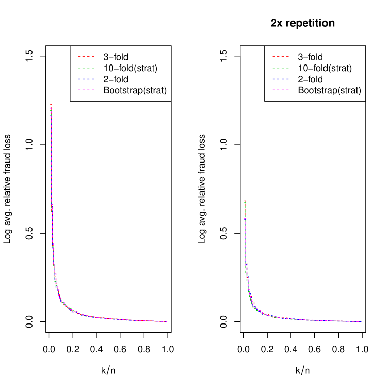
Figure 1: Plot of the log relative fraud loss as a function of the fraction $\tau=k/n$ of the observations that are selected, for a selection of the methods for setting the tuning parameter. The logistic regression model was used both to simulate the data, and to make predictions.

In Figure 1, the logarithm of the relative fraud loss is plotted as a function of the proportion $k/n$ of cases that are selected, for a selection of the validation procedures. From these, we see that there is not a very large difference between the different types. Further, it is hardest to select the best cases for lower values of $k/n$, as expected.

We repeat this experiment for the same datasets, but instead of estimating the probabilities using a penalised logistic regression model, we use an additive tree model fitted by boosting. The penalty parameter to be selected, is now the total number $M$ of components of the additive tree model. The average relative fraud loss for the different ways of choosing the number of iterations is reported in Table 3, and the logarithm of the relative fraud loss is plotted as a function of $k/n$ in Figure 2. Compared to the ridge regression fits, the relative fraud loss is now greater, meaning that the selected model differs more in size, compared to the minimum for each value of $k$. The best alternative now seems to be the bootstrap variants, with stratified 3-fold cross validation being the closest contender.

Table 3: Relative fraud loss averaged over all values of $k$, for data simulated from the linear model with $p=100$ $n=1000$, and fitted with an additive tree model.

Notes	10-fold cv	5-fold cv	3-fold cv	2-fold cv	Bootstrap
	1.2060	1.1779	1.1617	1.1424	1.1578
stratified	1.2123	1.1716	1.1534	1.1403	1.1496
2x repeat	1.0586	1.0507	1.0526	1.0541	1.0464
2x repeat, stratified	1.0552	1.0523	1.0499	1.0515	1.0472

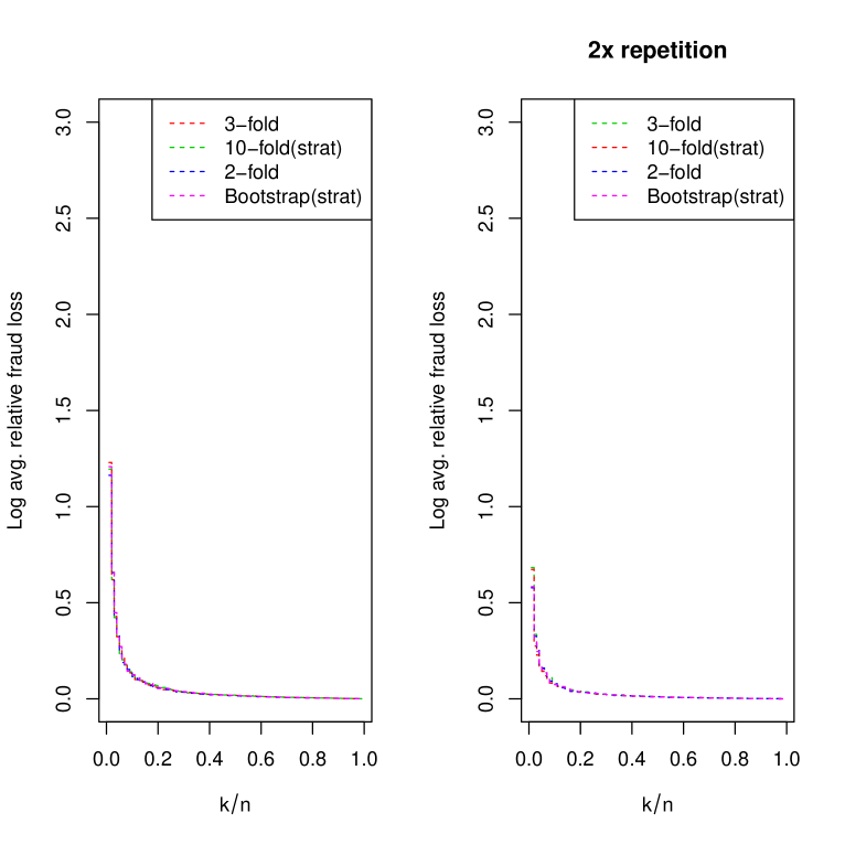
Figure 2: Plot of the relative fraud loss as a function of the fraction $\tau=k/n$ of the observations that are selected, for a selection of the methods for setting the tuning parameter. The logistic regression model was used both to simulate the data, and the additive tree model to make predictions.

5.3 Data drawn from an additive tree model

Next, we do a similar experiment, the difference being the model that the data are drawn from. Instead of a logistic regression model, we draw from a model where the linear predictor is replaced with an additive tree model, as previously outlined. We first estimate models using penalised logistic regression.

Table 4: Relative fraud loss averaged over all values of $k$, for data simulated from the additive tree model with $p=100$ $n=1000$, and fitted with the linear model.

Notes	10-fold cv	5-fold cv	3-fold cv	2-fold cv	Bootstrap
	1.0190	1.0195	1.0193	1.0189	1.0194
stratified	1.0199	1.0195	1.0191	1.0190	1.0193
2x repeat	1.0197	1.0193	1.0193	1.0190	1.0199
2x repeat, stratified	1.0196	1.0195	1.0192	1.0193	1.0196

The results of this are summarised in Table 4.

Table 5: Relative fraud loss averaged over all values of $k$, for data simulated from the additive tree model with $p=100$ $n=1000$, and fitted with the additive tree model.

Notes	10-fold cv	5-fold cv	3-fold cv	2-fold cv	Bootstrap
	1.0463	1.0450	1.0452	1.0454	1.0450
stratified	1.0469	1.0474	1.0457	1.0451	1.0454
2x repeat	1.0467	1.0464	1.0456	1.0435	1.0451
2x repeat, stratified	1.0473	1.0453	1.0464	1.0450	1.0452

We also estimate additive tree models, the results for which are summarised in Table 5. In the first case, 2-fold cross-validation gave the best results, with stratified 3-fold cross validation in second place. Curiously, the error does not seem to be smaller when doubling the number of repetitions, which could suggest that it is easier to select the best model for the data simulated from a more complex model. For the latter case, 2-fold cross validation seems to be the best option, based on the average relative fraud loss. It could be argued that real data are most likely to follow a model that is more complex than a logistic regression model with a linear predictor, and therefore that repeated 2-fold cross validation is the more reliable option, overall.

5.4 Comparison with an alternative approach

Next, we want to compare our approach to other relevant methods. One such method is to set the penalty parameter using the AUC as a criterion. This is a popular measure for assessing the performance of a binary regression model in terms of discrimination. It is also related to ranking, and is therefore a natural alternative to fraud loss. In fact, the AUC can on a population level be seen to be equivalent to the probability that an observation where $Y=0$ will be given a lower probability than one where $Y=1$. Hence, if one model has a higher AUC than another, then the aforementioned probability will be highest for the model with the highest AUC [5]. Symbolically, this can be written as

$$\text{AUC}\left(\hat{p}\right) =P\left(\hat{p}(x_{i})\geq\hat{p}(x_{j})|Y_{i}=1,Y_{j}=0\right),$$

which may be estimated by the Wilcoxon type statistic

$$\widehat{\text{AUC}}=\frac{\sum_{i=1}^{n}\sum_{j=1}^{n}(1-y_{i})y_{j}\mathcal{I}\left(\hat{p}(\mathbf{x}_{j})>\hat{p}(\mathbf{x}_{i})\right)}{\sum_{i=1}^{n}y_{i}\sum_{i=1}^{n}(1-y_{i})}.$$

Table 6: Relative fraud loss averaged over $k$ for the methods based on the AUC and the fraud loss, for data simulated with $p=100$ $n=1000$.

Simulation model	Logistic	Logistic	Additive trees	Additive trees
Estimation model	Logistic	Additive trees	Logistic	Additive trees
Average over all $K=10,20,\dots 990$:
auc	1.0335	1.0763	1.0186	1.0482
fraud	1.0371	1.0741	1.0195	1.0442
auc, 2x repeat	1.0337	1.0730	1.0183	1.0470
fraud, 2x repeat	1.0350	1.0721	1.0186	1.0454
Average over $K=160,170,\dots 240,250$:
auc	1.0349	1.0626	1.0228	1.0583
fraud	1.0356	1.0591	1.0232	1.0531
auc, 2x repeat	1.0338	1.0610	1.0228	1.0570
fraud, 2x repeat	1.0359	1.0601	1.0225	1.0545

The log-likelihood function, or likelihood-based measures, such as the Akaike information criterion (AIC), are also commonly used to set tuning parameters, but we will here disregard these. However, they are not particularly relevant for the problem, as we are not interested in finding the model that gives the best fit to all the data. Further, the log-likelihood function often explodes numerically when some of the probabilities become very close to $1$. In our experiments, this happened often during cross validation when we evaluated the log-likelihood function for the data that were not used for estimation.

The first simulations are based on the same models as previously discussed, using 2-fold cross validation with and without repetition in both methods. Table 6 reports the resulting average fraud loss. The average over a smaller range of values of $k/n=0.16,0.17,\dots,0.25,$ which is realistic in practice for the fraud setting is also shown in the table. When looking at the average over $k/n$ from $0.01$ to $0.99$, it seems that it is advantageous to select the model complexity via the cross validated fraud loss when estimating an additive tree model, whatever the data generating model is. When we only consider an aggregate over values of $k/n$ from $0.16$ to $0.25$, we see the same, and in addition there also seems to be a slight benefit to using the fraud loss, when fitting penalised logistic regression models to data simulated from an additive tree model.

In Figure 3, the average difference in fraud loss for the two approaches applied to the data simulated from logistic regression models, is plotted as a function of $k/n.$ It seems that in neither case, one or the other method is consistently better across the entire grid over $k/n$. However, there is a tendency, especially when $k/n$ is larger than roughly $0.2$, that the fraud loss works best when estimating an additive tree model, but not when estimating a penalised logistic regression model. Figure 4 is a similar plot, but where the data are simulated from the additive tree model. It seems, in this case, that the fraud loss is more favourable when a penalised logistic regression model is estimated, compared to when the data were simulated from the logistic regression model.

Figure 3: Plot of the difference in fraud loss when selecting the model complexity according to the AUC and the fraud loss, respectively. The data are simulated from the logistic regression model with $n=1000$ and $p=100$.

Figure 4: Plot of the difference in fraud loss when selecting the model complexity according to the AUC and the fraud loss, respectively. The data are simulated from additive tree model with $n=1000$ and $p=100$.

We repeat the experiment, but we now expand the datasets so that the number of covariates is $p=n=1000.$ These are simulated in the same way as for $p=100.$ We again simulate data both from a logistic regression model, and from an additive tree model, and scale the number of covariates that the response depends on with the dimension of the covariate matrix, so that it in both cases depends on $150$ covariates. For the logistic regression model, the $150$ non-zero effects take values in the interval $(-0.67,0.85),$ and the average absolute value of these is $0.198.$ A comparison of the two approaches for selecting the model complexity, in all four combinations of data-generating and estimated model, is summarised in terms of the average relative fraud loss in Table 7. The average relative fraud loss over the whole range of $k/n$ is now lowest when using the approach based on the fraud loss, except when both the data-generating and the estimated model are logistic. When we only look at the average over $k/n=0.16,\dots,0.25,$ it seems to be beneficial to select the model complexity with the fraud loss in all cases, although the difference between the results from the two methods is quite small when estimating a penalised regression model.

Figure 5 is a plot corresponding to Figure 3, but for $p=1000.$ The fraud loss is now lowest overall, when the tuning parameter is selected with the cross validated fraud loss for the boosted models, but not for the penalised logistic regression models. When the data are simulated from an additive tree model, as shown in Figure 6, there seems to be an advantage to using the fraud loss when estimating penalised regression models, at least for $k/n$ up to $0.2$. Fraud loss also seems to be best for the boosted tree models, perhaps except when $k/n<0.2$, possibly due to a high variance. These results could indicate that it is better to chose the penalty parameter by cross validating the fraud loss, than by the AUC, when the model is misspecified.

Table 7: Relative fraud loss averaged over $k$ for the methods based on the AUC and the fraud loss, for data simulated with $p=1000$ $n=1000$.

Simulation model	Logistic	Logistic	Additive trees	Additive trees
Estimation model	Logistic	Additive trees	Logistic	Additive trees
Average over all $k=10,20,\dots 990$:
auc	1.0338	1.0925	1.0232	1.0572
fraud	1.0352	1.0919	1.0218	1.0537
auc, 2x repeat	1.0337	1.0991	1.0239	1.0559
fraud, 2x repeat	1.0351	1.0910	1.0216	1.0539
Average over $k=160,170,\dots 240,250$:
auc	1.0394	1.0875	1.0287	1.0729
fraud	1.0375	1.0824	1.0316	1.0683
auc, 2x repeat	1.0389	1.0920	1.0301	1.0705
fraud, 2x repeat	1.0387	1.0847	1.0294	1.0693

Figure 5: Plot of the difference in fraud loss when selecting the model complexity according to the AUC and the fraud loss, respectively. The data are simulated from the logistic regression model with $n=1000$ and $p=1000$. covariates.

Figure 6: Plot of the difference in fraud loss when selecting the model complexity according to the AUC and the fraud loss, respectively. The data are simulated from the additive tree model with $n=1000$ and $p=1000$. covariates.

Table 8: Relative fraud loss averaged over $k$ for the methods based on the AUC and the fraud loss, for data simulated with $p=4000$ $n=1000$.

Simulation model	Logistic	Logistic	Additive trees	Additive trees
Estimation model	Logistic	Additive trees	Logistic	Additive trees
Average over all $k=10,20,\dots 990$:
auc	1.0415	1.0526	1.0229	1.0453
fraud	1.0400	1.0577	1.0182	1.0457
auc, 2x repeat	1.0412	1.0520	1.0229	1.0443
fraud, 2x repeat	1.0388	1.0547	1.0187	1.0438
Average over $k=160,170,\dots 240,250$:
auc	1.0538	1.0605	1.0187	1.0507
fraud	1.0498	1.0655	1.0223	1.0585
auc, 2x repeat	1.0532	1.0567	1.0189	1.0491
fraud, 2x repeat	1.0468	1.0591	1.0239	1.0530

Figure 7: Plot of the difference in fraud loss when selecting the model complexity according to the AUC and the fraud loss, respectively. The data are simulated from the logistic regression model with $n=1000$ and $p=4000$. covariates.

Figure 8: Plot of the difference in fraud loss when selecting the model complexity according to the AUC and the fraud loss, respectively. The data are simulated from the additive tree model with $n=1000$ and $p=4000$. covariates.

We repeat the experiment again, now in a context where $p>n$. Specifically, we let $p=4000,$ while we keep the number of observations at $n=1000.$ With the exception of the correlation matrix $R$, the model parameters are scaled up in the same way as when the number of covariates was changed from $100$ to $1000$. The correlation matrix is now constructed from one $(1000)\times(1000)$ correlation matrix that is stacked diagonally, giving a block-diagonal correlation matrix where $4\times{10}^{6}$ out of the $16\times{10}^{6}$ entries are non-zero. When the data are simulated from the logistic regression model, we see in Figure 8 that picking the tuning parameter for a penalised logistic regression model using the fraud loss, generally works better than the AUC, at least when $k/n<0.4,$ and that for the boosted trees it seems to be consistently worse, or at least not better. For the data drawn from an additive tree model, the fraud loss is better for values of $k/n$ up to about $0.12$ for the penalised logistic regression models, with more or less no difference for $k/n>0.4.$ For the boosted trees, the fraud loss performs somewhat worse for values of $k/n$ up to about $0.3.$ All of the simulations are summed up in Table 8, demonstrating that the fraud loss on average performs better than the AUC for the penalised logistic regression models, regardless of whether the data are simulated from a logistic regression model or an additive tree model when we look at the entire range of $k$. If we only look at $k/n=0.16,0.17,\dots,0.25$, the fraud loss performs better only for penalised logistic regression when the data are drawn from a logistic regression model.

All in all, selecting the model complexity by cross validating the fraud loss seems to work quite well, compared to using the AUC, especially for values of $k/n$ close to the marginal probability of $Y$. This is good, as one could argue that these are the most interesting values in most fraud detection applications. The fraud loss does not outperform the AUC in all cases, such as for the boosted tree models for $p>n$, or the penalised regression models when the data are simulated from a logistic regression model, and $p<n$. A possible explanation for the first case could be that when estimating the probabilities is difficult due to $p>n,$ and the data generating model is complex, then trying to adapt the model locally to $k/n$, as in the method using the fraud loss, could introduce instability. For the latter case, it could be that the estimation problem is so simple that one more or less recovers the data generating model, and that there might not be too much to gain from adapting the model to a specific $k/n$.

6 Illustration on VAT fraud data

In this section, we will consider a dataset of controlled cases of potential VAT fraud from the Norwegian Tax Administration (Skatteetaten). The data are sensitive. Therefore, they have been somewhat manipulated in order to be anonymised, and very little meta-information, such as what the covariates represent, is included. The data were collected in 39 different 2-month periods, and include in total around $n=50000$ observations of $p=555$ covariates, where $20$ of the covariates are binary, $12$ are categorical, and $523$ are numerical. We recode the categorical covariates as binary variables, which then effectively gives us $p=616$ covariates. There are some missing values in the dataset. In order to be able to fit penalised logistic regression models, we impute the median for the missing values of the numerical variables. For the categorical variables, we instead recode them with an extra level that corresponds to a missing observation.

This dataset serves as an example of one particular case, where selecting the top cases is relevant. As an illustration, we take the data from the six 2-month periods leading up to, but not including, the 12th 2-month period as a training set, a total of $7843$ observations, out of which $1648$ are recorded as fraudulent. We use repeated 2-fold cross validation, with $9$ repetitions, to set the penalty parameter of a penalised logistic regression model, and the number of components in a boosted tree model. We set these parameters by cross validating the AUC and the fraud loss for $k/n=0.01,0.02,\dots,0.98,0.99.$ We then evaluate the models chosen by cross validation on the $1072$ observations collected in the 12th period, of which $216$ are recorded as fraudulent. The results of this is summed up in Table 9 and Figure 9, where the fraud loss is plotted as a function of $k/n$ for both the models, and both of the ways of setting the tuning parameter. For the penalised logistic regression models, it is evident from Figure 9 that the models chosen by the fraud loss are better than the model chosen by the AUC, at least up to around $k/n\approx 0.3,$ while for the boosted trees it is harder to see a clear difference between the two. The reported figures in Table 9 show that the fraud loss performs better, both in terms of the average relative fraud loss aggregated over $k/n=0.01,0.02,\dots,0.99$, and over the smaller selection of values $k/n=0.16,0.17,\dots,0.25,$ for both of the models. The absolute figures reported in parentheses also show that penalised logistic regression in this case gave somewhat lower fraud loss than the boosted trees, which indicates that this model is perhaps a little better suited for the given setting.

Table 9: Relative aggregated fraud loss, with aggregated fraud loss given in parentheses. Comparison of AUC and fraud loss. Dataset of VAT fraud from the Norwegian tax administration.

Estimation model	Logistic	Additive trees
Average over all $k/n=0.01,0.02,\dots 0.99$:
auc	1.0412 (0.6974)	1.0328 (0.6948)
fraud	1.0276 (0.6911)	1.0285 (0.6930)
Average over $k/n=0.16,0.17,\dots 0.24,0.25$:
auc	1.0854  (0.6361)	1.0301 (0.6244)
fraud	1.0609 (0.6218)	1.0269 (0.6225)

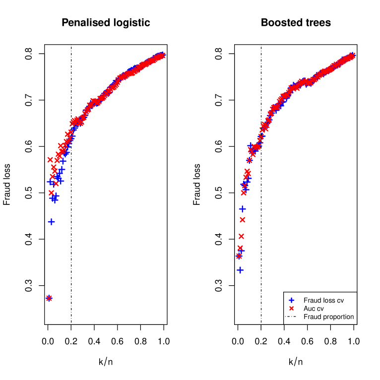
Figure 9: Plot of the fraud loss when selecting the model according to the AUC and fraud loss, respectively. Dataset of VAT fraud from the Norwegian Tax Administration.

7 Concluding remarks

Statistical fraud detection consists in creating a system, that automatically selects a subset of the cases that should be manually investigated. However, the investigator is often limited to controlling a restricted number $k$ of cases. In order to allocate the resources in the most efficient manner, one should then try to select the $k$ cases with the highest probability of being fraudulent. Prediction models that are used for this purpose, must typically be regularised to avoid overfitting. In this paper, we propose a new loss function, the fraud loss, for selecting the complexity of the prediction model via a tuning parameter. More specifically, we suggest an approach where either a penalised logistic regression model, or an additive tree model is fitted by maximising the log-likelihood of a binary regression model with a logit-link, and the tuning parameter is set by minimising the fraud loss function.

In a simulation study, we have investigated different ways of selecting the model complexity with the fraud loss, taking the out-of-sample performance into account, either by cross validation or bootstrapping. Based on this, repeated cross validation with few folds seems to be the most favourable. In particular, we have opted for repeated 2-fold cross validation without stratification. Still, we recognise that stratification might be necessary if there are very few cases of fraud in the training data.

Then, we carried out a larger simulation study, where we compared the performance of setting tuning parameters by cross validating the fraud loss, to cross validating the AUC. In these simulations, we saw that the fraud loss gave the best results in most cases, particularly when the proportion of the cases we to select is close to the marginal probability of fraud.

We have also illustrated our approach on a dataset of VAT fraud from the Norwegian Tax Administration, making the same comparison as in the second round of simulations. In this example, the fraud loss performed better than the AUC, most substantially when fitting penalised logistic regression models, which were also the model that were the most adequate for this application.

We have focussed on two particular estimation methods and corresponding definitions of the model complexity. The first is maximising the logistic log-likelihood function, subject to ridge regularisation, where the penalty parameter is the one to be chosen. The second is boosting for an additive tree model, where the number of trees is the focus. The first could however be easily adapted to the other types of regularisation, such as the lasso or the elastic net. For the second, one might define the complexity in terms of for instance the size of each tree. One could also imagine using the fraud loss to select the complexity for other types of binary classification models. Further, one might search for new divergences to optimise that put more emphasis on estimating the higher probabilities accurately, which is similar the the work of Rudin [18], Boyd et al. [2] and Eban et al. [7]. Another alternative is to adapt regression trees to the problem of picking a certain number of cases. This might be done by fitting small trees directly combined with bagging, or by pruning a decision tree to minimise the fraud loss after growing the tree using a standard splitting criterion.

8 Acknowledgements

This work is funded by The Research Council of Norway centre Big Insight, Project 237718. The authors would also like to thank Riccardo De Bin, for his useful input, and participation in discussions.

References

- Bolton and Hand [2002] Richard J Bolton and David J Hand. Statistical fraud detection: A review. Statistical Science, 17(3):235–249, 2002.
- Boyd et al. [2012] Stephen Boyd, Corinna Cortes, Mehryar Mohri, and Ana Radovanovic. Accuracy at the top. In F. Pereira, C. J. C. Burges, L. Bottou, and K. Q. Weinberger, editors, Advances in Neural Information Processing Systems 25, pages 953–961. Curran Associates, Inc., 2012. URL http://papers.nips.cc/paper/4635-accuracy-at-the-top.pdf.
- Chen and Guestrin [2016] Tianqi Chen and Carlos Guestrin. Xgboost: A scalable tree boosting system. In Proceedings of the 22nd acm sigkdd international conference on knowledge discovery and data mining, pages 785–794. ACM, 2016.
- Clémençon and Vayatis [2007] Stéphan Clémençon and Nicolas Vayatis. Ranking the best instances. Journal of Machine Learning Research, 8(Dec):2671–2699, 2007.
- Clémençon et al. [2008] Stéphan Clémençon, Gábor Lugosi, Nicolas Vayatis, et al. Ranking and empirical minimization of u-statistics. The Annals of Statistics, 36(2):844–874, 2008.
- Dorogush et al. [2018] Anna Veronika Dorogush, Vasily Ershov, and Andrey Gulin. Catboost: gradient boosting with categorical features support. arXiv preprint arXiv:1810.11363, 2018.
- Eban et al. [2016] Elad ET Eban, Mariano Schain, Alan Mackey, Ariel Gordon, Rif A Saurous, and Gal Elidan. Scalable learning of non-decomposable objectives. arXiv preprint arXiv:1608.04802, 2016.
- Efron [1983] Bradley Efron. Estimating the error rate of a prediction rule: improvement on cross-validation. Journal of the American statistical association, 78(382):316–331, 1983.
- Efron and Tibshirani [1997] Bradley Efron and Robert Tibshirani. Improvements on cross-validation: the 632+ bootstrap method. Journal of the American Statistical Association, 92(438):548–560, 1997.
- Freund et al. [2003] Yoav Freund, Raj Iyer, Robert E Schapire, and Yoram Singer. An efficient boosting algorithm for combining preferences. Journal of machine learning research, 4(Nov):933–969, 2003.
- Friedman [2001] Jerome H Friedman. Greedy function approximation: a gradient boosting machine. Annals of statistics, pages 1189–1232, 2001.
- Hoerl and Kennard [1970] Arthur E Hoerl and Robert W Kennard. Ridge regression: Biased estimation for nonorthogonal problems. Technometrics, 12(1):55–67, 1970.
- Joachims [2005] Thorsten Joachims. A support vector method for multivariate performance measures. In Proceedings of the 22nd international conference on Machine learning, pages 377–384. ACM, 2005.
- Joe [2006] Harry Joe. Generating random correlation matrices based on partial correlations. Journal of Multivariate Analysis, 97(10):2177–2189, 2006.
- Ke et al. [2017] Guolin Ke, Qi Meng, Thomas Finley, Taifeng Wang, Wei Chen, Weidong Ma, Qiwei Ye, and Tie-Yan Liu. Lightgbm: A highly efficient gradient boosting decision tree. In Advances in Neural Information Processing Systems, pages 3146–3154, 2017.
- Nelsen [2007] Roger B Nelsen. An introduction to copulas. Springer Science & Business Media, 2007.
- Robertson and Zaragoza [2007] Stephen Robertson and Hugo Zaragoza. On rank-based effectiveness measures and optimization. Information Retrieval, 10(3):321–339, 2007.
- Rudin [2009] Cynthia Rudin. The p-norm push: A simple convex ranking algorithm that concentrates at the top of the list. Journal of Machine Learning Research, 10(Oct):2233–2271, 2009.
- Tibshirani [1996] Robert Tibshirani. Regression shrinkage and selection via the lasso. Journal of the Royal Statistical Society: Series B (Methodological), 58(1):267–288, 1996.
- Zou and Hastie [2005] Hui Zou and Trevor Hastie. Regularization and variable selection via the elastic net. Journal of the royal statistical society: series B (statistical methodology), 67(2):301–320, 2005.