Eccentric binary black hole surrogate models for the gravitational waveform and remnant properties: comparable mass, nonspinning case

Abstract

We develop new strategies to build numerical relativity surrogate models for eccentric binary black hole systems, which are expected to play an increasingly important role in current and future gravitational-wave detectors. We introduce a new surrogate waveform model, NRSur2dq1Ecc, using 47 nonspinning, equal-mass waveforms with eccentricities up to $0.2$ when measured at a reference time of $5500M$ before merger. This is the first waveform model that is directly trained on eccentric numerical relativity simulations and does not require that the binary circularizes before merger. The model includes the $(2,2)$, $(3,2)$, and $(4,4)$ spin-weighted spherical harmonic modes. We also build a final black hole model, NRSur2dq1EccRemnant, which models the mass, and spin of the remnant black hole. We show that our waveform model can accurately predict numerical relativity waveforms with mismatches $\approx 10^{-3}$, while the remnant model can recover the final mass and dimensionless spin with absolute errors smaller than $\approx 5\times 10^{-4}M$ and $\approx 2\times 10^{-3}$ respectively. We demonstrate that the waveform model can also recover subtle effects like mode-mixing in the ringdown signal without any special ad-hoc modeling steps. Finally, we show that despite being trained only on equal-mass binaries, NRSur2dq1Ecc can be reasonably extended up to mass ratio $q\approx 3$ with mismatches $\simeq 10^{-2}$ for eccentricities smaller than $\sim 0.05$ as measured at a reference time of $2000M$ before merger. The methods developed here should prove useful in the building of future eccentric surrogate models over larger regions of the parameter space.

I Introduction

Detection of gravitational waves (GWs) Abbott et al. (2019a, 2020a) by the LIGO Aasi et al. (2015) and Virgo Acernese et al. (2015) detectors has opened a new window in astrophysics to probe binary compact objects – binary black holes (BBHs) being the most abundant source for these detectors. Both detection and extraction of source properties from the GW signal relies on the availability of accurate inspiral-merger-ringdown (IMR) waveform models for BBHs. While numerical relativity (NR) provides the most accurate gravitational waveforms for BBHs, they are computationally expensive, taking weeks to months to generate a single waveform. Data-driven surrogate modeling strategies Field et al. (2014); Pürrer (2014); Blackman et al. (2015, 2017a, 2017b); Varma et al. (2019a); Chua et al. (2019); Lackey et al. (2019); Varma et al. (2019b); Williams et al. (2020); Khan and Green (2020); Haegel and Husa (2020) have been shown to be capable of producing waveforms that are nearly indistinguishable from NR with evaluation times of less than $0.1$ seconds. While NR surrogate waveform models for nonspinning Blackman et al. (2015), aligned-spin Varma et al. (2019a), and precessing BBHs Blackman et al. (2017b); Varma et al. (2019b) are well developed, NR surrogate modeling of eccentric systems is completely unexplored.

So far, all GW detections of BBHs are consistent with signals emitted from quasicircular binaries Abbott et al. (2019b); Romero-Shaw et al. (2019); Lenon et al. (2020); Yun et al. (2020); Wu et al. (2020); Nitz et al. (2019); Ramos-Buades et al. (2020a). In fact, eccentricity has been traditionally ignored in most GW data analyses (for e.g. Refs. Abbott et al. (2020a, 2019a)). This is motivated by the expectation that even if a binary is formed with a non-zero eccentricity, it should circularize before reaching the frequency band of ground based detectors, as eccentricity gets radiated away via GWs during the long inspiral Peters (1964). However, this assumption may not always hold, especially for binaries formed in dense environments like globular clusters or galactic nuclei Giesler et al. (2018); Rodriguez et al. (2018a); O’Leary et al. (2006); Samsing (2018); Fragione and Kocsis (2019); Kumamoto et al. (2019); O’Leary et al. (2009); Gondán and Kocsis (2020). Indeed, recent follow-up analysis of GW190521 Abbott et al. (2020b) claim this event to be consistent with a BBH source with eccentricity ranging from $\sim 0.1$ Romero-Shaw et al. (2020) up to $\sim 0.7$ Gayathri et al. (2020) (see also Calderón Bustillo et al. (2020a, b)).

Eccentricity, if present in GW signals, carries precious astrophysical information about the environment in which the binary was formed. The detection of an eccentric merger would not only be a smoking-gun signature of sources formed via dynamical encounters, but would point towards specific type of interactions, namely GW captures Zevin et al. (2019), taking place in those environments. Catching eccentric sources in the mHz regime targeted by the LISA space mission is also a promising avenue to distinguish astrophysical formation channels Nishizawa et al. (2017, 2016); Breivik et al. (2016); Fang et al. (2019); Rodriguez et al. (2018b); Gondán et al. (2018); Tagawa et al. (2020).

Furthermore, ignoring eccentricity in our models can lead to systematic biases if the actual signal corresponds to an eccentric system Ramos-Buades et al. (2020b). Such biases can also lead to eccentric systems being misidentified as a violation of general relativity (GR). Even if all binaries are found to be circular, eccentric models are necessary to place bounds on the eccentricity. Therefore, including eccentricity in our GW models is important, especially as the detectors become more sensitive.

In the last few years, a handful of eccentric inspiral-only Klein et al. (2018); Tiwari and Gopakumar (2020); Moore et al. (2018); Moore and Yunes (2019); Liu et al. (2020); Tanay et al. (2019) and IMR models Hinderer and Babak (2017); Hinder et al. (2018); Huerta et al. (2018); Chen et al. (2020); Chiaramello and Nagar (2020); Cao and Han (2017) have become available. We highlight some recent eccentric IMR models in the following. ENIGMA Huerta et al. (2018); Chen et al. (2020) is a nonspinning eccentric BBH model that attaches an eccentric post-Newtonian (PN) inspiral to a quasicircular merger based on an NR surrogate model Blackman et al. (2015). SEOBNRE Cao and Han (2017) modifies an aligned-spin quasicircular EOB waveform model Taracchini et al. (2012) to include some effects of eccentricity. Similarly, Ref. Chiaramello and Nagar (2020) modifies a different aligned-spin EOB multipolar waveform model for quasicircular BBHs Nagar et al. (2018, 2020) to include some effects of eccentricity. The model is then further improved by replacing the carrier quasicircular model with a generic eccentric one Nagar et al. (2021). In addition to these models, Ref. Setyawati and Ohme (2021) recently developed a method to add eccentric modulations to existing quasicircular BBH models.

Notably, all of these models rely on the assumption that the binary circularizes by the merger time. While this is approximately true for many expected sources Huerta et al. (2018); Habib and Huerta (2019), this necessarily places a limit on the range of validity of these models. In addition, none of these models are calibrated on eccentric NR simulations, even though their accuracy is tested by comparing against eccentric simulations.

Apart from the waveform prediction, BBH remnant modeling from eccentric sources is also of crucial astrophysical importance Sperhake et al. (2008); Hinder et al. (2008); Sopuerta et al. (2007); Sperhake et al. (2020). For example, recoils from eccentric mergers can be up to $25\%$ higher than the circular case Sopuerta et al. (2007); Sperhake et al. (2020), which result in a higher likelihood of ejections from astrophysical hosts like star clusters and galaxies.

It is, therefore, timely to invest in building faithful eccentric BBHs waveform and remnant models that address some of these limitations. In this paper, we develop a detailed framework for constructing a surrogate model with eccentric NR data. We then build a two-dimensional surrogate model, NRSur2dq1Ecc, over parameters that describe eccentricity for equal-mass, nonspinning systems to demonstrate the efficacy of the proposed methods. This is the first eccentric waveform that is directly trained on eccentric NR simulations and does not need to assume that the binary circularizes before merger. The model can produce waveforms that are of comparable accuracy to the NR simulations used to train it. Furthermore, despite being trained only on equal-mass eccentric BBHs, we find that the model can be reasonably evaluated beyond its training range upto mass ratio $q\approx 3$ provided the eccentricities are small.

In addition to the waveform model, we build a surrogate model for the remnant mass and spin, NRSur2dq1EccRemnant, which can provide accurate predictions for the final state of eccentric binary mergers. This work paves the way forward for building future eccentric surrogate models: we expect that the methods developed here can be applied straightforwardly to aligned-spin eccentric BBHs, while the precessing case requires significantly more work.

The rest of the paper is organized as follows. Sec. II describes the NR simulations. Sec. III describes data decomposition, parameterization and construction of the surrogate model. In Sec. IV, we test the surrogate model by comparing against NR waveforms. We end with some concluding remarks in Sec. V.

II Numerical Relativity Data

NR simulations for this work are performed using the Spectral Einstein Code (SpEC) SpE developed by the Simulating eXterme Spacetimes (SXS) collaboration SXS . We follow the procedure outlined in Ref. Chatziioannou et al. (2021) to construct initial orbital parameters that result in a desired eccentricity. The constraint equations are solved employing the extended conformal thin sandwich formalism York (1999); Pfeiffer and York (2003) with superposed harmonic Kerr free data Varma et al. (2018). The evolution equations are solved employing the generalized harmonic formulation Lindblom et al. (2006); Rinne et al. (2009). The time steps during the simulations are chosen nonuniformly using an adaptive time-stepper Boyle et al. (2019). Further details can be found in Ref. Boyle et al. (2019) and references within. We perform 47 new eccentric NR simulations that have been assigned the identifiers SXS:BBH:2266 - SXS:BBH:2312, and will be made available through the SXS public catalog SXS Collaboration .

The component BH masses, $m_{1}$ and $m_{2}$, and dimensionless spins, $\bm{\chi}_{1}$ and $\bm{\chi}_{2}$, are measured on the apparent horizons Boyle et al. (2019) of the BHs, where index 1 (2) corresponds to the heavier (lighter) BH. The component masses at the relaxation time Boyle et al. (2019) are used to define the mass ratio $q=m_{1}/m_{2}\geq 1$ and total mass $M=m_{1}+m_{2}$. Unless otherwise specified, all masses in this paper are given in units of the total mass. When training the surrogate model, we restrict ourselves to $q=1$, $\bm{\chi}_{1},\bm{\chi}_{2}=0$ in this work.

The waveform is extracted at several extraction spheres at varying finite radii from the origin and then extrapolated to future null infinity Boyle et al. (2019); Boyle and Mroue (2009). These extrapolated waveforms are then corrected to account for the initial drift of the center of mass Boyle (2016, ). The spin-weighted spherical harmonic modes at future null infinity, scaled to unit mass and unit distance, are denoted as $\mathpzc{h}_{\ell m}(t)$ in this paper.

The complex strain $\mathpzc{h}=h_{+}-ih_{\times}$ is given by:

$$\mathpzc{h}(t,\iota,\varphi_{0})=\sum^{\infty}_{\ell=2}\sum_{m=-l}^{l}\mathpzc{h}_{\ell m}(t)\leavevmode\nobreak\ _{-2}Y_{\ell m}(\iota,\varphi_{0}),$$ (1)

where $h_{+}$ ($h_{\times}$) is the plus (cross) polarization of the waveform, ${}_{-2}Y_{\ell m}$ are the spin$\,=\!\!-2$ weighted spherical harmonics, and $\iota$ and $\varphi_{0}$ are the polar and azimuthal angles on the sky in the source frame. We model modes with $(\ell,m)={(2,2),(3,2),(4,4)}$. Because of the symmetries of equal-mass, nonspinning BBHs, all odd-$m$ modes are identically zero, and the $m<0$ modes can be obtained from the $m>0$ modes. Therefore, we model all non-zero $\ell\leq 3$ and $(4,\pm 4)$ modes, except the $m=0$ modes. We exclude $m=0$ memory modes because (non-oscillatory) Christodoulou memory is not accumulated sufficiently in our NR simulations Favata (2009); this defect was recently addressed in both Cauchy characteristic extraction (CCE) Mitman et al. (2020a); Barkett et al. (2020); Moxon et al. (2020) and extrapolation Mitman et al. (2020b) approaches. The $(4,2)$ mode, on the other hand, was found to have significant numerical error in the extrapolation procedure Boyle et al. (2019); Boyle and Mroue (2009). We expect this issue to be resolved with CCE as well. Therefore, in future models, we should be able to include the $m=0$ modes as well as modes like the (4,2) mode.

The remnant mass $m_{f}$ and spin $\bm{\chi}_{f}$ are determined from the common apparent horizon long after the ringdown, as described in Ref. Boyle et al. (2019). For nonprecessing systems like the ones considered here, the final spin is directed along the direction of the orbital angular momentum. Unlike previous surrogate models Varma et al. (2019b, c, 2020), we do not model the recoil kick in this work, as the symmetries of equal-mass, nonspinning BBHs restrict the kick to be zero.

III Surrogate methodology for eccentric waveforms

In this section, we describe our new framework to build NR surrogate models for eccentric BBHs. We begin by applying the following post processing steps that simplify the modeling procedure.

III.1 Processing the training data

In order to construct parametric fits (cf. Sec. III.4) for the surrogate model, it is necessary to align all the waveforms such that their peaks occur at the same time. We define the peak of each waveform, $\tau_{peak}$, to be the time when the quadrature sum,

$$A_{\rm tot}(\tau)=\sqrt{\sum_{l,m}|\mathpzc{h}_{\ell m}(\tau)|^{2}}\,,$$ (2)

reaches its maximum. Here the summation is taken over all the modes being modeled. We then choose a new time coordinate,

$$t=\tau-\tau_{\rm peak}\,,$$ (3)

such that $A_{\rm tot}(t)$ for each waveform peaks at $t=0$.

Next, we use cubic splines to interpolate the real and imaginary parts of the waveform modes onto a common time grid of [$-5500M$, $75M$] with a uniform time spacing of $dt=0.1M$; this is dense enough to capture all frequencies of interest, including near merger. The initial time of $-5500M$ is chosen so that we can safely eliminate spurious initial transients in the waveform, also known as junk radiation Boyle et al. (2019), for each waveform in our dataset.

Once all the waveforms are interpolated onto a common time grid, we perform a frame rotation of the waveform modes about the z-axis such that the orbital phase is zero at $t=-5500M$. The orbital phase is obtained from the $(2,2)$ mode [cf. Eq. (14)]. Because of the symmetry of the equal-mass, equal-spin systems considered here, the odd-$m$ modes are identically zero and so we need not worry about remaining $\phi_{\rm orb}\rightarrow\phi_{\rm orb}+\pi$ rotational freedom as was necessary in Refs. Blackman et al. (2015, 2017a, 2017b); Varma et al. (2019a, b). This preprocessing of time and phase ensures that the waveform varies smoothly across the parameter space, which in turn makes modeling easier.

III.2 Measuring eccentricity and mean anomaly

Departure of NR orbits from circularity is measured by a time-dependent eccentricity and mean anomaly. Eccentricity takes values between $[0,1]$ where the boundary values correspond to a quasicircular binary and an unbound orbit Chandrasekhar (1998), respectively. Mean anomaly, on the other hand, is bounded by $[0,2\pi)$. While it may seem most natural to estimate orbital parameters from the BH trajectories, this task is complicated by the fact that any such measurement will be impacted by the gauge conditions chosen by the NR simulation. We instead choose to estimate eccentricity and anomaly parameters directly from the waveform data at future null infinity.

III.2.1 Measuring eccentricity

Various methods to extract the eccentricity from NR simulations have been proposed in the literature Habib and Huerta (2019); Healy et al. (2017); Mroue et al. (2010); Purrer et al. (2012). As the eccentricity evolves during the binary’s orbit Peters (1964), these methods use dynamical quantities such as some combination of the $(2,2)$ mode’s amplitude, phase, or frequency. All of these methods reduce to the eccentricity parameter in the Newtonian limit. The estimated value of the eccentricity may differ slightly depending on the method used and the noise in the numerical data. However, as long as they provide a consistent measurement of eccentricity that decays monotonically with time, one can use any of the eccentricity estimators for constructing a surrogate waveform model. For this work, we use the following definition of eccentricity based on orbital frequency Mora and Will (2002):

$$e(t)=\frac{\sqrt{\omega_{p}(t)}-\sqrt{\omega_{a}(t)}}{\sqrt{\omega_{p}(t)}+\sqrt{\omega_{a}(t)}},$$ (4)

where $\omega_{a}$ and $\omega_{p}$ are the orbital frequencies at apocenter (i.e. point of furthest approach) and pericenter (i.e. point of closest approach), respectively. Unlike several other eccentricity estimators proposed in literature Habib and Huerta (2019); Healy et al. (2017); Mroue et al. (2010); Purrer et al. (2012), the one defined in Eq. (4) is normalized and reduces to the eccentricity parameter in the Newtonian limit at both low and high eccentricities Ramos-Buades et al. (2020b).

We first compute the orbital frequency,

$$\omega_{\rm orb}=\frac{d\phi_{\mathrm{\rm orb}}}{dt}\,,$$ (5)

where $\phi_{\mathrm{\rm orb}}$ is the orbital phase inferred from the (2,2) mode (cf. Eq. (14)), and the derivative is approximated using second-order finite differences. We then find the times where $\omega_{\rm orb}$ passes through a local maxima (minima) and associate those to pericenter (apocenter) passages, to obtain $\omega_{p}$ ($\omega_{a}$). We find that using the local maxima/minima of the amplitude of the $(2,2)$ mode to identify the pericenter/apocenter times leads to a consistent value for the eccentricity. We then interpolate $\omega_{p}$ and $\omega_{a}$ onto the full time grid using cubic splines. This gives us $\omega_{p}(t)$ and $\omega_{a}(t)$, which are used in Eq. (4).

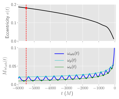
Figure 1: Time evolution of the eccentricity $e(t)$ (upper panel) and the orbital frequency $\omega_{\rm orb}(t)$ (lower panel) for NR Simulation SXS:BBH:2304. $\omega_{p}$ and $\omega_{a}$ denote, respectively, the the orbital frequency at pericenter (local maxima, cyan circles) and apocenter passages (local minima, green circles). From this data we construct spline interpolants to obtain $\omega_{p}(t)$ (cyan curve) and $\omega_{a}(t)$ (green curve). The eccentricity is then estimated using Eq. (4). The red dashed vertical line corresponds to the reference time $t_{\rm ref}=-5500M$ at which the surrogate model is parameterized.

Figure 1 shows an example of the measured eccentricity for the NR simulation SXS:BBH:2304. We see that our method provides a smooth, monotonically decreasing $e(t)$. The estimate become unreliable near merger where finding local maxima/minima in $\omega_{\rm orb}$ becomes problematic as the orbit transitions from inspiral to plunge. The estimate also becomes problematic whenever the eccentricity is extremely small, thereby preventing the appearance of an identifiable local maxima/minima. This does not affect our modeling, however, as we only require an eccentricity value at a reference time while the binary is still in the inspiral phase. We select a reference time of $t_{\rm ref}=-5500M$ and parameterize our waveform model by

$$e_{\rm ref}=e(t_{\rm ref})\,.$$ (6)

While estimating $e_{\rm ref}$, we include the data segment slightly before $t_{\rm ref}$ as this allows us to interpolate, rather than extrapolate, when constructing $e(t)$ in Eq. (4).

III.2.2 Measuring mean anomaly

In the Newtonian context, the mean anomaly $l$ of an eccentric orbit is defined as

$$l \equiv 2\pi\frac{t-t_{0}}{P},$$ (7)

where $t_{0}$ is a time corresponding to the previous pericenter passage and $P$ is the radial period, which is defined to be the time between two successive pericenter passages. In the Newtonian case $P$ is a constant, but in GR it changes as the binary inspirals. However, one can continue to use Eq. (7) as a meaningful measurement of the radial oscillation’s phase for the purpose of constructing a waveform model Hinder et al. (2018).

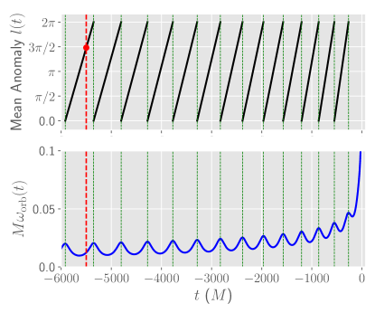
Figure 2: Time evolution of the mean anomaly $l(t)$ (upper panel) and the orbital frequency $\omega_{\rm orb}(t)$ (lower panel) for the NR Simulation SXS:BBH:2304. Green dashed vertical lines indicate the times for pericenter passages. The anomaly $l(t)$ grows linearly with time over $[0,2\pi)$ in between two successive pericenters. The red dashed vertical line corresponds to the reference time $t_{\rm ref}=-5500M$ at which the surrogate model is parametrized.

For each NR waveform, we compute the times for all pericenter passages using the same procedure as in Sec. III.2.1. We divide the time array into different orbital windows defined as $[t_{i}^{\rm peri},t_{i+1}^{\rm peri})$, where $t_{i}^{\rm peri}$ is the time for $i^{th}$ pericenter passage. The orbital period in each window is given by $P_{i}=t_{i+1}^{\rm peri}-t_{i}^{\rm peri}$, and the mean anomaly by

$$l_{i}(t)=2\pi\frac{t-t_{i}^{\rm peri}}{P_{i}}\,.$$ (8)

Note that each $l_{i}(t)$ grows linearly with time over $[0,2\pi)$ for the window $[t_{i}^{\rm peri},t_{i+1}^{\rm peri})$. To obtain the full $l(t)$, we simply join each $l_{i}(t)$ for consecutive orbits. Finally, the value for mean anomaly parameterizing our waveform model is then simply the evaluation of the mean anomaly at $t_{\rm ref}=-5500M$.

$$l_{\rm ref}=l(t_{\rm ref})\,.$$ (9)

Figure 2 shows an example application of our method to estimate the mean anomaly of the NR simulation SXS:BBH:2304.

III.2.3 Targeted parameter space

In Fig. 3, we show the measured values for eccentricity and mean anomaly at $t_{\rm ref}$ for all 47 NR waveforms, which leads to the following 2d parameter space for our model:

• eccentricity: $e_{\rm ref}\in[0,0.2]$;

• mean anomaly: $l_{\rm ref}\in[0,2\pi)$.

Fig. 3 shows a large gap in the parameter space, which reflects an inherent limitation in our current approach to achieve target eccentricity parameters from the initial data. The method we use to construct initial orbital parameters Chatziioannou et al. (2021) seeks to achieve target values of $(e_{\rm ref},l_{\rm ref})$ at a time $500M$ after the start of the simulation. The initial orbital frequency is chosen such that time to merger is $6000M$, as predicted by a leading-order PN calculation. Unfortunately, this is only approximate, leading to different merger times for different simulations. Consequently, when we estimate the eccentricity parameters at $t_{\rm ref}=-5500M$, this is no longer a fixed time from the start of the simulation. The eccentricity parameters evolve differently for different simulations during this time, leading to the clustering in Fig. 3. In the future, we plan to resolve this using a higher order PN expression, or an eccentric waveform model Huerta et al. (2018); Chen et al. (2020); Chiaramello and Nagar (2020) to predict the time to merger.

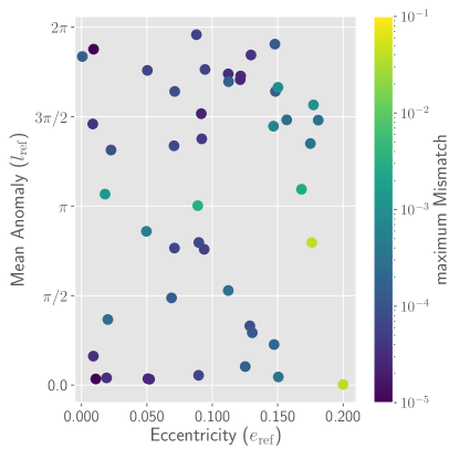
Figure 3: The parameter space covered by the 47 NR waveforms (circle markers) used in the construction of our surrogate model. The axes show the eccentricity and mean anomaly values at $t_{\rm ref}$. We also show the dependence of the maximum (over the sky of the source frame) flat-noise mismatches on the parameters eccentricity and mean anomaly (cf. Sec. IV.1.2). The colors indicate the maximum mismatch, which systematically increases near the high eccentricity boundary where few training data points are available.

III.3 Waveform data decomposition

Building a surrogate model becomes more challenging for oscillatory and complicated waveform data. One solution is to transform or decompose the waveform data into several simpler “waveform data pieces” that also vary smoothly over the parameter space. These simpler data pieces can then be modeled more easily and recombined to get back the original waveform. Successful decomposition strategies have been developed for quasi-circular NR surrogates Blackman et al. (2015); Varma et al. (2019a, b); Blackman et al. (2017a, b). In order to develop similar strategies for eccentric waveform data, we have pursued a variety of options. We now summarize the most successful decomposition technique we have tried, while relegating some alternatives to Appendix A.

III.3.1 Decomposing the quadrupolar mode $\mathpzc{h}_{22}$

The complex $(2,2)$ waveform mode,

$$\mathpzc{h}_{22}=A_{22}\leavevmode\nobreak\ e^{-\mathrm{i}\phi_{22}}\,,$$ (10)

can be decomposed into an amplitude, $A_{22}$, and phase, $\phi_{22}$. For non-precessing systems in quasicircular orbit, $A_{22}$ and $\phi_{22}$ are slowly varying functions of time, and have therefore been used as waveform data pieces for many modeling efforts. For eccentric waveforms, however, both amplitude and phase show highly oscillatory modulations on the orbital time scale (cf. Figs. 1 and 2 for the frequency, which is a time-derivative of the phase). This demands further decomposition of the waveforms into even simpler data pieces. One natural solution could have been to build interpolated functions of the local maxima and minima of $A_{22}$ and $\phi_{22}$. The secular trend of these functions can then be subtracted out from the original amplitude and phase. The resulting residual amplitude and phase data may be easier to model. Unfortunately, as mentioned in Sec. III.2.1, finding the local maxima/minima becomes problematic near the merger.

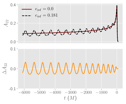
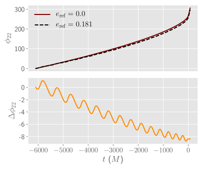
Figure 4: Example decomposition of the amplitude and phase of the $(2,2)$ mode. Upper left: Amplitude $A_{22}$ of the eccentric waveform SXS:BBH:2304 (with eccentricity $e_{\rm ref}=0.181$) along with the amplitude $A_{22}^{0}$ of the noneccentric waveform SXS:BBH:1155. Lower left: The residual amplitude $\Delta A_{22}=A_{22}-A_{22}^{0}$. Upper right: Phase $\phi_{22}$ of the eccentric waveform SXS:BBH:2304 and the phase $\phi_{22}^{0}$ of the noneccentric waveform SXS:BBH:1155. Lower right: The residual phase $\Delta\phi_{22}=\phi_{22}-\phi_{22}^{0}$. In this work we model $\Delta A_{22}$ and $\Delta\phi_{22}$

We instead follow a simpler approach whereby the amplitude and phase of a quasicircular $q=1$, nonspinning NR waveform (SXS:BBH:1155) is used as a proxy for the secular trend of the amplitude and phase. We then compute the residual amplitude and phase,

$$\Delta A_{22}=A_{22}-A_{22}^{0},$$ (11)

$$\Delta\phi_{22}=\phi_{22}-\phi_{22}^{0},$$ (12)

where $A_{22}^{0}$ and $\phi_{22}^{0}$ are the amplitude and phase of the noneccentric waveform, respectively, which have been aligned according the same procedure outlined in Sec. III.1. In the upper-left panel of Fig. 4, we show the amplitude of an eccentric waveform (SXS:BBH:2304) along with the amplitude of its noneccentric counterpart (SXS:BBH:1155) which traces the secular trend of the nonmonotonically increasing eccentric amplitude. The difference of these two amplitudes, $\Delta A_{22}$, is then plotted in the lower-left panel. $\Delta A_{22}$ is simpler to model than $A_{22}$, as it isolates the oscillatory component of $A_{22}$. Similarly, in the right panels of Fig. 4, we show the phase evolution of the same eccentric waveform (SXS:BBH:2304), its noneccentric counterpart (SXS:BBH:1155), and their difference $\Delta\phi_{22}$ which isolates the oscillatory component of $\phi_{22}$. Note that noneccentric waveform data is plentiful Boyle et al. (2019) and accurate surrogate models have been built for noneccentric NR waveforms Varma et al. (2019a, b). So extending the residual amplitude and phase computation to spinning, unequal-mass systems is straightforward. For instance the surrogate model of Ref. Varma et al. (2019a) can be used to generate $A_{22}^{0}$ and $\phi_{22}^{0}$ for generic aligned-spin systems.

III.3.2 Decomposing the higher order modes

In this paper, we model the quadrupolar mode and the higher-order modes differently. For $\mathpzc{h}_{22}$, we model data pieces closely associated with the amplitude and phase as described above. On the other hand, for higher order modes, we first transform the waveform into a co-orbital frame in which the waveform is described by a much simpler and slowly varying function. This is done by applying a time-dependent rotation given by the instantaneous orbital phase:

$$\mathpzc{h}_{\ell m}^{C}=\mathpzc{h}_{\ell m}\leavevmode\nobreak\ e^{\mathrm{i}m\phi_{\mathrm{orb}}},$$ (13)

$$\phi_{\mathrm{orb}}=\frac{\phi_{22}}{2},$$ (14)

where $\phi_{22}$ is the phase of the $(2,2)$ mode (cf. Eq. (10)), $\phi_{\mathrm{orb}}$ is the orbital phase, and $\mathpzc{h}_{\ell m}^{C}$ represents the complex modes in the co-orbital frame.

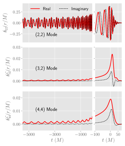
Figure 5: The waveform modes for NR Simulation SXS:BBH:2304 ($e_{\rm ref}=0.181$) are shown. The top panel shows the dominant $(2,2)$ mode in the inertial frame. Two higher-order modes $(3,2)$ and $(4,4)$ in the co-orbital frame are shown in the middle and lower panels respectively. The waveform is aligned such that the peak of the amplitude occurs at $t=0$ and the orbital phase is zero at $t_{\rm ref}=-5500M$.

We use the real and imaginary parts of $\mathpzc{h}_{\ell m}^{C}$ as our waveform data pieces for the nonquadrupole modes. As shown in Fig. 5, the $\mathpzc{h}_{\ell m}^{C}$ data have less structure, making them easier to model. We find that using quasicircular $\mathpzc{h}_{\ell m}^{C}$ to subtract off the secular trend does not provide any modeling advantage. We, therefore, model the real and imaginary parts of $\mathpzc{h}_{\ell m}^{C}$ without any further data decomposition.

III.3.3 Summary of waveform data pieces

To summarize, the full set of waveform data pieces we model is as follows: $\Delta A_{22}$, $\Delta\phi_{22}$ for the (2,2) mode, and real and imaginary parts of $\mathpzc{h}_{\ell m}^{C}$ for the (3,2) and (4,4) modes.

III.4 Building the waveform model

We decompose the inertial frame waveform data into many waveform data pieces as summarized in Sec. III.3.3. For each of these data pieces, we now build a surrogate model using reduced basis, empirical interpolation, and parametric fits across the parameter space. The detailed procedure is outlined in Refs. Blackman et al. (2017b); Field et al. (2014), which we only briefly describe here.

For each waveform data piece, we employ a greedy algorithm to construct a reduced basis Field et al. (2011) such that the projection errors (cf. Eq. (5) of Ref. Blackman et al. (2017b)) for the entire data set onto this basis are below a given tolerance. We use a basis tolerance of $10^{-2}$ radians for $\Delta\phi_{22}$ , $1.5\times 10^{-3}$ for $\Delta A_{22}$ and $2\times 10^{-5}$ for the real part of $\mathpzc{h}_{32}^{C}$. For all other data pieces, basis tolerance is set to $5\times 10^{-5}$.

These choices are made so that we include sufficient number of basis functions for each data piece [9 for $\Delta A_{22}$, 12 for $\Delta\phi_{22}$, 7 (5) for the real (imaginary) part of $\mathpzc{h}_{32}^{C}$ and 10 (6) for the real (imaginary) part of $\mathpzc{h}_{44}^{C}$] to capture the underlying physical features in the simulations while avoiding over fitting. We perform additional visual inspection of the basis functions to ensure that they are not noisy in which case modeling accuracy can become comprised (cf. Appendix B of Ref. Blackman et al. (2017b)).

The next step is to construct an empirical interpolant in time using a greedy algorithm which picks the most representative time nodes Maday et al. (2009); Chaturantabut and Sorensen (2010); Field et al. (2014); Canizares et al. (2015). The number of the time nodes for each data piece is equal to the number of basis functions used. The final surrogate-building step is to construct parametric fits for each data piece at each of the empirical time nodes across the two-dimensional parameter space $\{e_{\rm ref},l_{\rm ref}\}$. We do this using the Gaussian process regression (GPR) fitting method as described in Refs. Taylor and Varma (2020); Varma et al. (2019c).

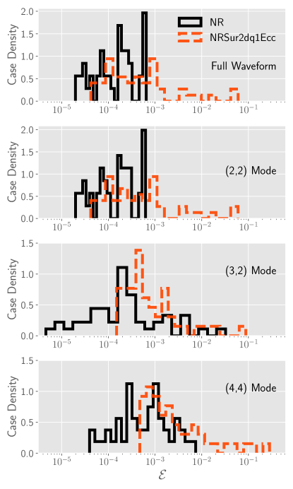
Figure 6: Time-domain leave-one-out errors $\mathcal{E}$, defined in Eq. (17), for the full waveform as well as the individual modes considered in the model. For comparison, we also show the NR error between the two highest resolutions. The largest errors are found near the parameter domain’s boundary where the trial surrogate, built as part of the cross-validation study, is extrapolating.

III.5 Evaluating the waveform surrogate

To evaluate the NRSur2dq1Ecc surrogate model, we provide the eccentricity $e_{\rm ref}$ and mean anomaly $l_{\rm ref}$ as inputs. We then evaluate the parametric fits for each waveform data pieces at each time node. Next, the empirical interpolant is used to reconstruct the full waveform data pieces (cf. Sec. III.3.3).

We compute the amplitude and phase of the $(2,2)$ mode,

$$A_{22}^{S}=\Delta A_{22}^{S}+A_{22}^{0},$$ (15)

$$\phi_{22}^{S}=\Delta\phi_{22}^{S}+\phi_{22}^{0},$$ (16)

where $\Delta A_{22}^{S}\approx\Delta A_{22}$ and $\Delta\phi_{22}^{S}\approx\Delta\phi_{22}$ are the surrogate models for $\Delta A_{22}$ and $\Delta\phi_{22}$ respectively while $A_{22}^{0}$ and $\phi_{22}^{0}$ are the amplitude and phase of the quasicircular NR waveform used in the decompositions [cf. Eqs. (11-12)]. We obtain the (2,2) mode complex strain as $\mathpzc{h}^{S}_{22}=A_{22}^{S}\leavevmode\nobreak\ e^{-\mathrm{i}\phi_{22}^{S}}$.

For the nonquadrupole modes, we similarly evaluate the surrogate models for the real and imaginary parts of the co-orbital frame waveform data pieces $\mathpzc{h}_{\ell m}^{C,S}\approx\mathpzc{h}_{\ell m}^{C}$ and treat it as $\mathpzc{h}_{\ell m}^{C}$. Finally, we use Eqs. (10), (13), and (14) to obtain the surrogate prediction for the inertial frame strain $\mathpzc{h}_{\ell m}^{S}$ for these modes.

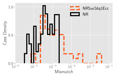
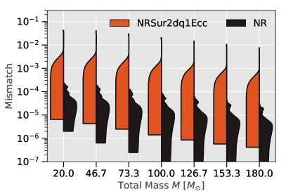
Figure 7: Left panel: Flat noise mismatch between the NRSur2dq1Ecc model (following the leave-one-out validation procedure) and the highest-resolution NR waveform data. For comparison, we also show the NR resolution error, obtained by comparing the two highest available resolutions. Right panel: NRSur2dq1Ecc (validation) mismatches computed using the advanced LIGO design sensitivity noise curve, as a function of the total mass of the binary. For comparison, we also show the NR mismatches. For each mass, the distribution of mismatches are shown as a smoothed vertical histogram (or a violin). The histograms are normalized so that all violins have equal width. The largest errors are found near the parameter domain’s boundary where the trial surrogate, built as part of the cross-validation study, is extrapolating.

III.6 Building the remnant surrogate

In addition to the waveform model, we also construct the first model for the remnant quantities of eccentric BBHs. The new remnant model, NRSur2dq1EccRemnant, predicts the final mass $m_{f}$ and the component of the final spin, $\chi_{fz}$, along the orbital angular momentum direction. The remnant model takes eccentricity $e_{\rm ref}$ and mean anomaly $l_{\rm ref}$ as its inputs and maps to the final state of the binary. The final mass and spin fits are also constructed using the GPR fitting method as described in Refs. Taylor and Varma (2020); Varma et al. (2019c).

IV Results

In this section we demonstrate the accuracy of NRSur2dq1Ecc and NRSur2dq1EccRemnant by comparing against the eccentric NR simulations described in Sec. II. We do this by performing a leave-one-out cross-validation study. In this study, we hold out one NR waveform from the training set and build a trial surrogate from the remaining 46 eccentric NR waveforms. We then evaluate the trial surrogate at the parameter value corresponding to the held out data, and compare its prediction with the highest-resolution NR waveform. We refer to the errors obtained by comparing against the left-out NR waveforms as cross-validation errors. These represent conservative error estimates for the surrogate models against NR. Since we have 47 eccentric NR waveforms, we build 47 trial surrogates for each error study. We compare these errors to the NR resolution error, estimated by comparing the two highest available NR simulations.

IV.1 NRSur2dq1Ecc errors

IV.1.1 Time domain error without time/phase optimization

In order to quantify the accuracy of NRSur2dq1Ecc, we first compute the normalized $L_{2}$-norm between the NR data and surrogate approximation

$$\mathcal{E}[\mathpzc{h},\mathpzc{\tilde{h}}]=\frac{1}{2}\frac{\sum_{\ell,m}\int_{t_{1}}^{t_{2}}|\mathpzc{h}_{\ell m}(t)-\mathpzc{\tilde{h}}_{\ell m}(t)|^{2}dt}{\sum_{\ell,m}\int_{t_{1}}^{t_{2}}|\mathpzc{h}_{lm}(t)|^{2}dt},$$ (17)

where $\mathpzc{h}(t)$ and $\tilde{\mathpzc{h}}(t)$ correspond to the complex strain for NR and NRSur2dq1Ecc waveforms, respectively. Here, $t_{1}$ and $t_{2}$ denote the start and end of the waveform data. As the NR waveforms are already aligned in time and phase, the surrogate reproduces this alignment. Therefore, we compute the time-domain error $\mathcal{E}$ without any further time/phase shifts.

In Fig. 6, we report both the full waveform and individual mode errors for NRSur2dq1Ecc. For comparison, we also show the NR resolution errors. When computing the full waveform error we use all modes included in the surrogate model $(\ell,m)=(2,2),(3,2),(4,4)$ in Eq. (17). To compute errors for individual modes, we restrict the sum in Eq. (17) to only the mode of interest. The NRSur2dq1Ecc errors are comparable to the NR errors in Fig. 6.

However, we find that the surrogate errors have an extended tail around two orders of magnitude larger than the largest NR mismatch. While this could imply over-fitting, we find that highest mismatches correspond to the parameter space adjacent to the higher eccentricity $e_{\rm ref}$ boundary where only few (to none) training waveforms are used. As will be discussed in Sec. IV.1.2, the sparsely sampled region of the training domain around $(e_{\rm ref}=0.2,l_{\rm ref}\lesssim 2)$ leads to this extended high-error tail in Fig. 6.

We further note in Fig. 6 that the highest error in each mode corresponds to the same point in the parameter space indicating consistency in our modeling. Furthermore, as we only deal with mass ratio $q=1$ waveforms, the contribution of the higher modes are expected to be negligible compared to the dominant $(2,2)$ mode (see for example, Ref. Varma and Ajith (2017)). Therefore, even though the $(3,3)$ and $(4,4)$ modes have larger relative errors compared to the $(2,2)$ mode, their contribution to the total error is much smaller. This can be verified by comparing the full waveform errors to the (2,2) mode errors in Fig. 6.

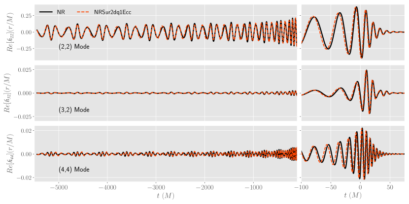
Figure 8: Real part of the waveform modes for the case that results in the largest flat noise mismatch ($\sim 0.04$) for NRSur2dq1Ecc (red dashed line) in the left panel of Fig 7. We also show the corresponding NR waveform, SXS:BBH:2308 (black solid line). The parameter values for this waveform are: $e_{\rm ref}=0.176$ and $l_{\rm ref}=2.51$. Note that this plot is generated using a trial surrogate that was not trained using this NR waveform data.

IV.1.2 Frequency domain mismatch with time/phase optimization

In this section, we estimate leave-one-out cross-validation errors by computing mismatches between the NR waveform and the trial surrogate waveform in the frequency domain. The frequency domain mismatch between two waveforms, $\mathpzc{h}_{1}$ and $\mathpzc{h}_{2}$ is defined as:

$$\left<\mathpzc{h}_{1},\mathpzc{h}_{2}\right>=4\mathrm{Re}\int_{f_{\mathrm{min}}}^{f_{\mathrm{max}}}\frac{\tilde{\mathpzc{h}}_{1}(f)\tilde{\mathpzc{h}}_{2}^{*}(f)}{S_{n}(f)}df,$$ (18)

where $\tilde{\mathpzc{h}}(f)$ indicates the Fourier transform of the complex strain $\mathpzc{h}(t)$, ^∗ indicates a complex conjugation, $\mathrm{Re}$ indicates the real part, and $S_{n}(f)$ is the one-sided power spectral density of a GW detector.

Before transforming the time domain waveform to the frequency domain, we first taper the time domain waveform using a Planck window McKechan et al. (2010), and then zero-pad to the nearest power of two. The tapering at the start of the waveform is done over $1.5$ cycles of the $(2,2)$ mode. The tapering at the end is done over the last $20M$. Once we obtain the frequency domain waveforms, we compute mismatches following the procedure described in Appendix D of Ref. Blackman et al. (2017b). The mismatches are optimized over shifts in time, polarization angle, and initial orbital phase. We compute the mismatches at 37 points uniformly distributed on the sky of the source frame, and use all available modes for the surrogate model.

We consider a flat noise curve $S_{n}(f)=1$ as well as the Advanced-LIGO design sensitivity Zero-Detuned-HighP noise curve from Ref. LIGO Scientific Collaboration (2018). We take $f_{\mathrm{min}}$ to be the frequency of the $(2,2)$ mode at the end of the initial tapering window while $f_{\mathrm{max}}$ is set at $4f^{\rm peak}_{22}$, where $f^{\rm peak}_{22}$ is the frequency of the $(2,2)$ mode at its peak. This ensures that the peak frequencies of all modes considered in our model are captured well, and we have confirmed that our mismatch values do not change for larger values of $f_{\mathrm{max}}$. Note that when computing mismatches using Advanced LIGO noise curve, for masses below $\sim 70M_{\odot}$, $f_{\mathrm{min}}$ is greater than $20$Hz, meaning that the signal starts within the detector sensitivity band.

The mismatches computed using the flat noise curve are shown in the left panel of Fig. 7. The histograms include mismatches for all 47 NR waveforms and source-frame sky locations. We find that the typical surrogate mismatches are $10^{-5}-10^{-3}$, which are comparable to but larger than the NR errors. As an example, Fig. 8 shows the surrogate and NR waveforms for the case that leads to the largest mismatch in the left panel of Fig. 7.

In Fig. 3, we show the dependence of the mismatches on the parameter space. It can be easily recognized that the surrogate yields largest errors at and around $(e_{\rm ref}=0.2,l_{\rm ref}\lesssim 2)$ where the training grid becomes sparse. Further, when these sparse data points themselves are left out when computing the cross-validation errors, the surrogate is effectively extrapolating in parameter space. This indicates that the surrogate accuracy could be improved by adding new NR simulations in this high-eccentricity region. However, achieving target values of $e_{\rm ref}$ and $l_{\rm ref}$ has proven difficult. We return to this issue in the conclusions.

The right panel of Fig. 7 shows the mismatches computed using advanced LIGO design sensitivity noise curve LIGO Scientific Collaboration (2018) for different total masses $M$ of the binary. For each $M$, we compute the mismatches for all 47 NR waveforms and source-frame sky locations and show the distribution of mismatches using vertical histograms known as violin plots. Over the mass range $20-180M_{\odot}$, the surrogate mismatches are at the level of $\sim 10^{-4}-10^{-3}$ but with an extending tail as before. However, we note that these errors are typically smaller than the mismatches for other eccentric waveform models Huerta et al. (2018); Chen et al. (2020); Chiaramello and Nagar (2020).

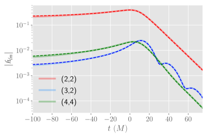
Figure 9: The absolute values of different spherical-harmonic modes are shown as dashed (solid) curves for the surrogate (NR) for SXS:BBH:2308, for which the surrogate produces largest flat noise mismatch ($\sim 0.04$). The parameter values for this waveform are: $e_{\rm ref}=0.176$ and $l_{\rm ref}=2.51$. Mode mixing for the $(3,2)$ mode is clearly seen in the ringdown signal of the NR waveform and is accurately reproduced by the surrogate.

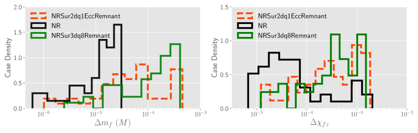
Figure 10: Leave-one-out error histograms of NRSur2dq1EccRemnant (red) for the remnant mass $m_{f}$ (left) and remnant spin $\chi_{fz}$ (right). For comparison we plot the NR errors (black), estimated by comparing the two highest resolution NR simulations, and errors for the noneccentric model NRSur3dq8cRemnant (green).

IV.2 Mode mixing

NR waveforms are extracted as spin-weighted spherical harmonic modes Newman and Penrose (1966); Goldberg et al. (1967). However, during the ringdown, the system can be considered a single Kerr black hole perturbed by quasinormal modes; perturbation theory tells us that the angular eigenfunctions for these modes are the spin-weighted spheroidal harmonics Teukolsky (1973, 1972). A spherical harmonic mode $\mathpzc{h}_{\ell m}$ can be written as a linear combination of all spheroidal harmonic modes with the same $m$ index. During the ringdown, each (spheroidal-harmonic) quasinormal mode decays exponentially in time, but each spherical-harmonic mode has a more complicated behavior because it is a superposition of multiple spheroidal-harmonic modes (of the same $m$ index) with different decay rates. This more complicated behavior is referred to as mode mixing, since power flows between different spherical-harmonic modes Berti and Klein (2014). This mixing is particularly evident in the $(3,2)$ mode as significant power of the dominant $(2,2)$ spherical-harmonic mode can leak into the $(3,2)$ spherical-harmonic mode. As the surrogate accurately reproduces the spherical harmonic modes from the NR simulations, it is also expected to capture the effect of mode mixing without any additional effort Varma et al. (2019a). We demonstrate this for an example case in Fig. 9 where we plot the amplitude of individual modes of the waveform during the ringdown. We show that the mode mixing in the $(3,2)$ mode is effectively recovered by the surrogate model.

IV.3 NRSur2dq1EccRemnant errors

In addition to the waveform surrogate, we also build a remnant surrogate model, NRSur2dq1EccRemnant, that predicts the mass and spin of the final BH left behind after the merger. This is the first such model for eccentric BBHs (but see e.g. Refs. Sopuerta et al. (2007); Sperhake et al. (2020)). Figure 10 shows the cross-validation errors of NRSur2dq1EccRemnant in predicting the remnant mass and spin. We find that NRSur2dq1EccRemnant can predict the final mass and spin with an accuracy of $\lesssim 5\times 10^{-4}M$ and $\lesssim 2\times 10^{-3}$ respectively. We further compute the errors for a noneccentric remnant model, NRSur3dq8Remnant Varma et al. (2019c), when compared against the same eccentric NR simulations, finding that errors in NRSur3dq8Remnant are comparable with NRSur2dq1EccRemnant errors. This suggests that noneccentric remnant models may be sufficient for equal-mass nonspinning binaries with eccentricities $e_{\rm ref}\leq 0.2$. However, we expect such models to disagree with eccentric simulations in the more general case of unequal-mass, spinning binaries (see for e.g. Ref. Ramos-Buades et al. (2020b)).

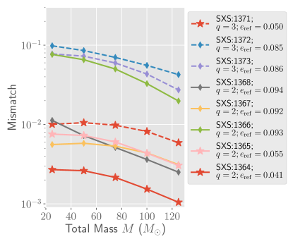
Figure 11: Mismatches against NR for the NRSur2dq1Ecc+ model (a simple extension of NRSur2dq1Ecc) when the surrogate is evaluated beyond its training parameter range ($q=1$). The mismatches are shown as a function of the binary total mass $M$ (at $\iota=\pi/3$, $\varphi_{0}=0.0$), and are computed using the advanced LIGO design sensitivity noise curve. We show mismatches for $q=2$ ($q=3$) as solid lines (dashed lines). We use star markers to denote waveforms with $e_{\rm ref}$ smaller than $\sim 0.05$ and diamond markers for the rest. All eccentricity values are computed at a reference time of $t_{\rm ref}=-2000M$.

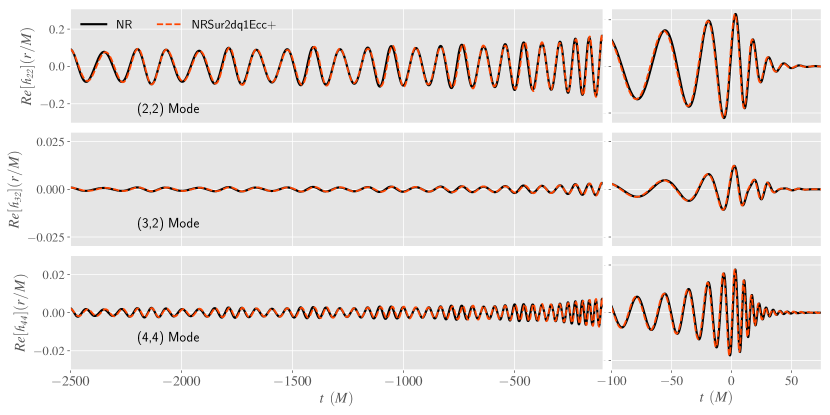
Figure 12: We show the NRSur2dq1Ecc+ prediction (red dashed line) beyond training range ($q=1$) of the surrogate for the case that results in the largest mismatch (Fig. 11) in the region defined by $e_{\rm ref}$ (at $t_{\rm ref}=-2000M$) smaller than $\sim 0.05$. We also show the corresponding NR waveform SXS:BBH:1371 (black solid line). The parameters for this waveform are: $q=3$, $e_{\rm ref}=0.050$ and $l_{\rm ref}=2.45$ (at $t_{\rm ref}=-2000M$).

IV.4 Extending NRSur2dq1Ecc to comparable mass systems

We now assess the performance of NRSur2dq1Ecc when evaluated beyond its training parameter range ($q=1$). To generate surrogate predictions at a given $(q,e_{\rm ref},l_{\rm ref})$, we first evaluate NRSur2dq1Ecc at $(q\!=\!1,e_{\rm ref},l_{\rm ref})$ and refer to the output as $\mathpzc{h}^{S}_{lm}(q\!=\!1,e_{\rm ref},l_{\rm ref})$. We then evaluate the noneccentric surrogate model NRHybSur3dq8 Varma et al. (2019a) at the given mass ratio $q$ and mass ratio $q=1$, and refer to the output as $\mathpzc{h}_{\ell m}^{0}(q)$ and $\mathpzc{h}_{\ell m}^{0}(q=1)$. We then compute the difference in amplitude and phase between $\mathpzc{h}^{S}_{lm}(q\!=\!1,e_{\rm ref},l_{\rm ref})$ and $\mathpzc{h}_{\ell m}^{0}(q=1)$:

$$\Delta A^{S}_{lm}(q\!=\!1,e_{\rm ref},l_{\rm ref})$$

$$\leavevmode\nobreak\ \leavevmode\nobreak\ \leavevmode\nobreak\ \leavevmode\nobreak\ \leavevmode\nobreak\ \leavevmode\nobreak\ \leavevmode\nobreak\ =A^{S}_{lm}(q\!=\!1,e_{\rm ref},l_{\rm ref})-A^{0}_{lm}(q\!=\!1)\,,$$ (19)

$$\Delta\phi^{S}_{lm}(q\!=\!1,e_{\rm ref},l_{\rm ref})$$

$$\leavevmode\nobreak\ \leavevmode\nobreak\ \leavevmode\nobreak\ \leavevmode\nobreak\ \leavevmode\nobreak\ \leavevmode\nobreak\ \leavevmode\nobreak\ =\phi^{S}_{lm}(q\!=\!1,e_{\rm ref},l_{\rm ref})-\phi^{0}_{lm}(q\!=\!1).$$ (20)

Even though these amplitude and phase differences are computed at $q=1$, we treat them as a proxy for the modulations due to eccentricity at any $q$. We then add these modulations to the amplitude and phase of $\mathpzc{h}_{\ell m}^{0}(q)$, the noneccentric surrogate model evaluated at the given $q$, to get the full amplitude and phase:

$$A^{S}_{lm}(q,e_{\rm ref},l_{\rm ref})$$

$$\leavevmode\nobreak\ \leavevmode\nobreak\ \leavevmode\nobreak\ \leavevmode\nobreak\ \leavevmode\nobreak\ \leavevmode\nobreak\ \leavevmode\nobreak\ \leavevmode\nobreak\ \leavevmode\nobreak\ =\Delta A^{S}_{lm}(q\!=\!1,e_{\rm ref},l_{\rm ref})+A^{0}_{lm}(q)\,,$$ (21)

$$\phi^{S}_{lm}(q,e_{\rm ref},l_{\rm ref})$$

$$\leavevmode\nobreak\ \leavevmode\nobreak\ \leavevmode\nobreak\ \leavevmode\nobreak\ \leavevmode\nobreak\ \leavevmode\nobreak\ \leavevmode\nobreak\ \leavevmode\nobreak\ \leavevmode\nobreak\ =\Delta\phi^{S}_{lm}(q\!=\!1,e_{\rm ref},l_{\rm ref})+\phi^{0}_{lm}(q).$$ (22)

The final surrogate prediction, which we view as a new, simple model NRSur2dq1Ecc+, is then:

$$\mathpzc{h}_{\ell m}^{S}(q,e_{\rm ref},l_{\rm ref})=A^{S}_{lm}(q,e_{\rm ref},l_{\rm ref})e^{-\mathrm{i}\phi^{S}_{lm}(q,e_{\rm ref},l_{\rm ref})}.$$ (23)

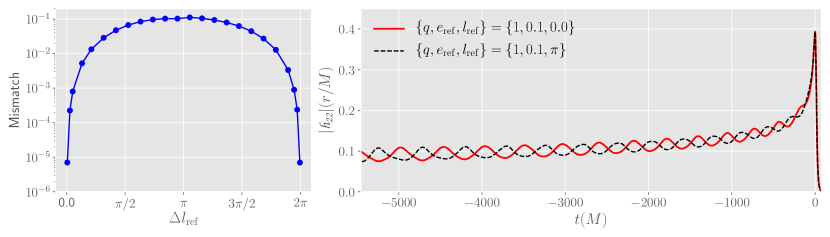
Figure 13: Importance of mean anomaly for waveform modeling and data analysis. Left panel: Flat noise mismatch (optimized over time, phase and polarization angle shifts) between NRSur2dq1Ecc predictions with $l_{\rm ref}=0.0$ and $l_{\rm ref}=\Delta l_{\rm ref}$, at fixed $q=1$ and $e_{\rm ref}=0.1$. While the mismatch, as expected, is $\sim 0$ for $\Delta l_{\rm ref}=0.0$ and $\Delta l_{\rm ref}=2\pi$, it reaches values $\sim 0.1$ near $\Delta l_{\rm ref}=\pi$. Right panel: The $(2,2)$ amplitude of the waveforms leading to the maximum mismatch, i.e. $l_{\rm ref}=0$ and $l_{\rm ref}=\pi$. These differences cannot be accounted for by a time or phase shift, therefore, mean anomaly is an important parameter to include for waveform modeling and data analysis of eccentric binaries.

To assess the accuracy of NRSur2dq1Ecc+ we compare against eight publicly available eccentric NR simulations with $q=2$ and $q=3$ Hinder et al. (2018); Boyle et al. (2019). These NR waveforms are shorter in length than the ones used to train our surrogate model. To ensure fair comparison between surrogate predictions and NR waveforms, we build a test surrogate which is parameterized by $e_{\rm ref}$ and $l_{\rm ref}$ at $t_{\rm ref}=-2000M$.

In Fig. 11, we show mismatches computed using the advanced LIGO design sensitivity noise curve, between the NRSur2dq1Ecc+ model and eccentric NR data at $q=2,3$. We include all modes available in the model while computing the mismatch. For simplicity, we only consider a single point in the source-frame sky, with an inclination angle of $\pi/3$. For $e_{\rm ref}$ (at $t_{\rm ref}=-2000M$) smaller than $\sim 0.05$, mismatches are always smaller than $10^{-2}$. As we increase $e_{\rm ref}$ (at $t_{\rm ref}=-2000M$) to $0.09$, the mismatches become significantly worse, especially for $q=3$, reaching values $\sim 10^{-1}$. As an example, Fig. 12 shows the surrogate prediction (and NR waveform) for the case that leads to the largest mismatch in Fig. 11 with $e_{\rm ref}$ (at $t_{\rm ref}=-2000M$) smaller than $\sim 0.05$.

This suggests that our scheme to extend the surrogate model to comparable mass systems produces reasonable waveforms for small eccentricities. However, we advise caution with extrapolation-type procedures in general.

IV.5 Importance of mean anomaly for data analysis

Many existing waveform models Huerta et al. (2018); Chen et al. (2020); Chiaramello and Nagar (2020); Cao and Han (2017) for eccentric binaries parameterize eccentric characteristics of the waveform by only one parameter $e_{\rm ref}$ while keeping $l_{\rm ref}$ fixed. We, however, use both $e_{\rm ref}$ and $l_{\rm ref}$ as parameters in our model. We find that not allowing $l_{\rm ref}$ as an independent parameter results in large modeling error, indicating that the mean anomaly is important to consider when modeling the GW signal from eccentric binaries.

To demonstrate the importance of mean anomaly also in data analysis, we present a simple study. We generate NRSur2dq1Ecc predictions $\mathpzc{h}_{\ell m}^{S}(q=1,e_{\rm ref}=0.1,l_{\rm ref})$ with $l_{\rm ref}\in[0.0,2\pi]$. The left panel of Fig. 13 shows mismatches between the waveform at $l_{\rm ref}=0$ and various $l_{\rm ref}$, parametrized by $\Delta l_{\rm ref}=l_{\rm ref}-0$. For simplicity, we only consider a single point in the source-frame sky, at $\iota=\pi/3$, $\varphi_{0}=0.0$. As expected, we find that $\Delta l_{\rm ref}=0.0$ and $\Delta l_{\rm ref}=2\pi$ produce identical waveforms. However, the mismatch reaches a value of $\sim 0.1$ at $\Delta l_{\rm ref}=\pi$. As we already account for allowed time and frame shifts when computing the mismatch, ignoring this difference can lead to modeling errors or biased parameter estimation. In the right panel of Fig. 13, we show the waveform amplitude for the cases with $l_{\rm ref}=0$ and $l_{\rm ref}=\pi$. The clear differences in the amplitude reinforce our assertion that this mismatch cannot be accounted for by a time or frame shift.

V Conclusion

We present NRSur2dq1Ecc, the first eccentric NR surrogate waveform model. This model is trained on 47 NR waveforms of equal-mass nonspinning BBH systems with eccentricity $e_{\rm ref}\leq 0.2$, defined at a reference time $t_{\rm ref}=-5500M$ before the waveform peak. The model includes the $(2,2)$, $(3,2)$ and $(4,4)$ spin-weighted spherical harmonic modes. Due to the symmetries of the equal-mass, nonspinning systems considered here, this is equivalent to including all $\ell\leq 3$ and $(4,\pm 4)$ modes, except the $m=0$ modes. This is the first eccentric BBH model that is directly trained on eccentric NR simulations and does not require that the binary circularizes before merger. We also present NRSur2dq1EccRemnant, the first NR surrogate model for the final BH properties of eccentric BBH mergers. This model is also trained on the same set of simulations. We use Gaussian process regression to construct the parametric fits for both models. Both NRSur2dq1Ecc and NRSur2dq1EccRemnant will be made publicly available in the near future.

Through a leave-one-out cross-validation study, we show that NRSur2dq1Ecc accurately reproduces NR waveforms with a typical mismatch of $\sim 10^{-3}$. We further demonstrate that our remnant model, NRSur2dq1EccRemnant, can accurately predict the final mass and spin of the merger remnant with errors $\lesssim 5\times 10^{-4}M$ and $\lesssim 2\times 10^{-3}$ respectively. We showed that despite being trained on equal-mass binaries, NRSur2dq1Ecc can be reasonably extended up to mass ratio $q\approx 3$ with mismatches $\simeq 10^{-2}$ for eccentricities $e_{\rm ref}\lesssim 0.05$ at $t_{\rm ref}=-2000M$. Finally, we demonstrate that the mean anomaly, which is often ignored in waveform modeling and parameter estimation of eccentric binaries, is an important parameter to include. Exclusion of mean anomaly can result in poor modeling accuracy and/or biased parameter inference.

The NR simulations used for this work were performed using the Spectral Einstein Code (SpEC) SpE . SpEC’s development efforts have been primarily focused on evolutions of binary black hole systems in quasi-circular orbits Boyle et al. (2019). To efficiently generate accurate training data for high eccentricity systems, it may be necessary to improve certain algorithmic subroutines. For example, as noted in Sec. III.2.3, we found it difficult to achieve target values of $(e_{\rm ref},l_{\rm ref})$ at a reference time before merger. We also noticed that the waveform’s numerical error was noticeably larger near pericenters, suggesting better adaptive mesh refinement algorithms Szilagyi et al. (2009) may be necessary for highly eccentric simulations.

We have also explored several data decomposition techniques and parametrizations for building eccentric NR surrogate models, which can guide strategies for future models. Our final framework for building eccentric NR surrogates is quite general, and we expect that it can be applied straightforwardly to higher dimensional parameter spaces including unequal masses and aligned-spins. We leave these explorations to future work.

Appendix

In this Appendix, we describe various alternate modeling strategies we pursued before deciding on the formalism presented in the main text.

Appendix A Choice of data decomposition

In this work, we have modeled the amplitude ($A_{22}$) and phase ($\phi_{22}$) of the $(2,2)$ mode by modeling the residual ($\Delta A_{22}$, $\Delta\phi_{22}$) of these quantities with respect to a quasicircular NR waveform (cf. Sec. III.3). Alternatively, one could instead model the amplitude and frequency (or their residuals), and then integrate the frequency to obtain the phase. The frequency of the (2,2) mode is given by

$$\omega_{22}=\frac{d\phi_{22}}{dt},$$ (24)

where $\phi_{22}$ is defined in Eq. (10). The corresponding residual is given by:

$$\Delta\omega_{22}=\omega_{22}-\omega_{22}^{0},$$ (25)

where $\omega_{22}^{0}$ is the frequency of $(2,2)$ mode for the quasicircular NR waveform.

We, therefore, explore four different data decomposition strategies for the $(2,2)$ mode, summarized below:

• Model $\{A_{22},\phi_{22}\}$ directly.

• Model $\{\Delta A_{22},\Delta\phi_{22}\}$ and then add them to the amplitude and phase of the quasicircular NR waveform to obtain $\{A_{22},\phi_{22}\}$.

• Model $\{A_{22},\omega_{22}\}$ and integrate the frequency data to get $\{A_{22},\phi_{22}\}$.

• Model $\{\Delta A_{22},\Delta\omega_{22}\}$; add them to the amplitude and frequency of the quasicircular NR waveforms, and finally integrate the frequency data to obtain $\{A_{22},\phi_{22}\}$.

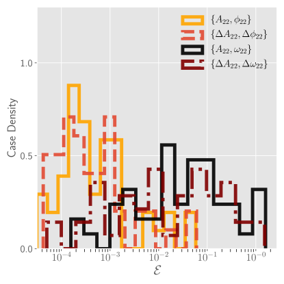
Figure 14: Histograms of surrogate errors (defined in Eqs. (17)) for the four different decomposition strategies we consider. We find that modeling the residual amplitude $\Delta A_{22}$ and residual phase $\Delta\phi_{22}$ yields the least errors.

In order to explore the effectiveness of these strategies, we build a separate surrogate model using each strategy. When building the frequency surrogates ($\omega_{22}$ or $\Delta\omega_{22}$) we use a basis tolerance of $10^{-3}$ rad/$M$. For $A_{22}$ ($\phi_{22}$) we use the same tolerance as used for $\Delta A_{22}$ ($\Delta\phi_{22}$) in Section III.4. We compute the normalized $L_{2}$-norm between the NR data and each surrogate approximation using Eq. (17). In Fig. 14, we show the surrogate errors for all four different strategies. We find that modeling the frequency $\omega_{22}$ or residual frequency $\Delta\omega_{22}$ yields at least two-to-three orders of magnitude larger $\mathcal{E}$ than when we model the phase $\phi_{22}$ or $\Delta\phi_{22}$. Furthermore, modeling the residual amplitude $\Delta A_{22}$ proves to be slightly more accurate than the case where we model the amplitude $A_{22}$ directly. Therefore, in the main text, we build surrogate models of the residual $\{\Delta A_{22},\Delta\phi_{22}\}$ (cf. Sec. III.3).

Appendix B Choice of fit parameterization

When building the surrogate models in main text, fits across parameter space are required for the waveform model as well as the remnant model (cf. Sec. III.4). These fits are parameterized by the eccentricity ($e_{\rm ref}$) and mean anomaly $(l_{\rm ref})$ at the reference time $t_{\rm ref}$. While $\{e_{\rm ref},l_{\rm ref}\}$ is a natural choice, we also explore the following choices of parameterizations:

• $\{e_{\rm ref},l_{\rm ref}\}$,

• $\{e_{\rm ref},\sin(l_{\rm ref}/2)\}$,

• $\{\log_{10}(1-e_{\rm ref}),l_{\rm ref}\}$,

• $\{\log_{10}(1-e_{\rm ref}),\sin(l_{\rm ref}/2)\}$,

Here $\sin(l_{\rm ref}/2)$ is considered because it maps the periodic parameter $l_{\rm ref}\in[0,2\pi)$ uniquely to the range $[0,1]$, while still mapping the physically equivalent points $l_{\rm ref}=0$ and $l_{\rm ref}=2\pi$ to the same point ($\sin(l_{\rm ref}/2)=0$). The same is not true for other possible parameterizations such as $\sin(l_{\rm ref})$, $\cos(l_{\rm ref})$, or $\cos(l_{\rm ref}/2)$. $\log_{10}(1-e_{\rm ref})$ is considered because it flattens the spread in eccentricity, which can be useful if the eccentricity varies over several orders of magnitude in the NR dataset.

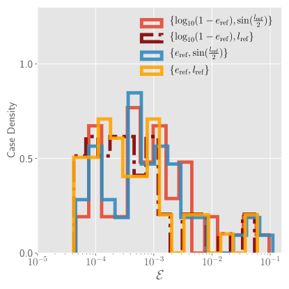
Figure 15: Histograms of the error for the full waveform, for the six different fit parameterizations we consider.

Similarly to the previous section, to explore the effectiveness of these strategies, we build a separate surrogate model using each strategy. Here, however, we consider all modes included $(\ell,m)=(2,2),(3,2),(4,4)$ and evaluate $\mathcal{E}$ errors [cf. Eq. (17)]. In Fig. 15, we show $\mathcal{E}$ errors for each parameterization strategy. We find that while the alternative strategies using either $\log_{10}(1-e_{\rm ref})$, or $\sin(l_{\rm ref}/2)$, or both, may be comparable, none of the them result in errors smaller than the original choice $\{e_{\rm ref},l_{\rm ref}\}$. As we do not achieve a noticeable improvement with these alternative parameterizations, we stick to the original choice $\{e_{\rm ref},l_{\rm ref}\}$ in the main text.

References

- Abbott et al. (2019a) B. P. Abbott et al. (LIGO Scientific, Virgo), “GWTC-1: A Gravitational-Wave Transient Catalog of Compact Binary Mergers Observed by LIGO and Virgo during the First and Second Observing Runs,” Phys. Rev. X9, 031040 (2019a), arXiv:1811.12907 [astro-ph.HE] .
- Abbott et al. (2020a) R. Abbott et al. (LIGO Scientific, Virgo), “GWTC-2: Compact Binary Coalescences Observed by LIGO and Virgo During the First Half of the Third Observing Run,” (2020a), arXiv:2010.14527 [gr-qc] .
- Aasi et al. (2015) J. Aasi et al. (LIGO Scientific), “Advanced LIGO,” Class. Quant. Grav. 32, 074001 (2015), arXiv:1411.4547 [gr-qc] .
- Acernese et al. (2015) F. Acernese et al. (Virgo), “Advanced Virgo: a second-generation interferometric gravitational wave detector,” Class. Quant. Grav. 32, 024001 (2015), arXiv:1408.3978 [gr-qc] .
- Field et al. (2014) S. E. Field, C. R. Galley, J. S. Hesthaven, J. Kaye, and M. Tiglio, “Fast Prediction and Evaluation of Gravitational Waveforms Using Surrogate Models,” 4, 031006 (2014), arXiv:1308.3565 [gr-qc] .
- Pürrer (2014) Michael Pürrer, “Frequency domain reduced order models for gravitational waves from aligned-spin compact binaries,” Class. Quant. Grav. 31, 195010 (2014), arXiv:1402.4146 [gr-qc] .
- Blackman et al. (2015) Jonathan Blackman, Scott E. Field, Chad R. Galley, Béla Szilágyi, Mark A. Scheel, Manuel Tiglio, and Daniel A. Hemberger, “Fast and Accurate Prediction of Numerical Relativity Waveforms from Binary Black Hole Coalescences Using Surrogate Models,” Phys. Rev. Lett. 115, 121102 (2015), arXiv:1502.07758 [gr-qc] .
- Blackman et al. (2017a) Jonathan Blackman, Scott E. Field, Mark A. Scheel, Chad R. Galley, Christian D. Ott, Michael Boyle, Lawrence E. Kidder, Harald P. Pfeiffer, and Béla Szilágyi, “Numerical relativity waveform surrogate model for generically precessing binary black hole mergers,” Phys. Rev. D96, 024058 (2017a), arXiv:1705.07089 [gr-qc] .
- Blackman et al. (2017b) Jonathan Blackman, Scott E. Field, Mark A. Scheel, Chad R. Galley, Daniel A. Hemberger, Patricia Schmidt, and Rory Smith, “A Surrogate Model of Gravitational Waveforms from Numerical Relativity Simulations of Precessing Binary Black Hole Mergers,” Phys. Rev. D95, 104023 (2017b), arXiv:1701.00550 [gr-qc] .
- Varma et al. (2019a) Vijay Varma, Scott E. Field, Mark A. Scheel, Jonathan Blackman, Lawrence E. Kidder, and Harald P. Pfeiffer, “Surrogate model of hybridized numerical relativity binary black hole waveforms,” Phys. Rev. D99, 064045 (2019a), arXiv:1812.07865 [gr-qc] .
- Chua et al. (2019) Alvin J.K. Chua, Chad R. Galley, and Michele Vallisneri, “Reduced-order modeling with artificial neurons for gravitational-wave inference,” Phys. Rev. Lett. 122, 211101 (2019), arXiv:1811.05491 [astro-ph.IM] .
- Lackey et al. (2019) Benjamin D. Lackey, Michael Pürrer, Andrea Taracchini, and Sylvain Marsat, “Surrogate model for an aligned-spin effective one body waveform model of binary neutron star inspirals using Gaussian process regression,” Phys. Rev. D 100, 024002 (2019), arXiv:1812.08643 [gr-qc] .
- Varma et al. (2019b) Vijay Varma, Scott E. Field, Mark A. Scheel, Jonathan Blackman, Davide Gerosa, Leo C. Stein, Lawrence E. Kidder, and Harald P. Pfeiffer, “Surrogate models for precessing binary black hole simulations with unequal masses,” Phys. Rev. Research. 1, 033015 (2019b), arXiv:1905.09300 [gr-qc] .
- Khan and Green (2020) Sebastian Khan and Rhys Green, “Gravitational-wave surrogate models powered by artificial neural networks: The ANN-Sur for waveform generation,” (2020), arXiv:2008.12932 [gr-qc] .
- Williams et al. (2020) Daniel Williams, Ik Siong Heng, Jonathan Gair, James A. Clark, and Bhavesh Khamesra, “Precessing numerical relativity waveform surrogate model for binary black holes: A Gaussian process regression approach,” Phys. Rev. D 101, 063011 (2020), arXiv:1903.09204 [gr-qc] .
- Abbott et al. (2019b) B.P. Abbott et al. (LIGO Scientific, Virgo), “Search for Eccentric Binary Black Hole Mergers with Advanced LIGO and Advanced Virgo during their First and Second Observing Runs,” Astrophys. J. 883, 149 (2019b), arXiv:1907.09384 [astro-ph.HE] .
- Romero-Shaw et al. (2019) Isobel M. Romero-Shaw, Paul D. Lasky, and Eric Thrane, “Searching for Eccentricity: Signatures of Dynamical Formation in the First Gravitational-Wave Transient Catalogue of LIGO and Virgo,” Mon. Not. Roy. Astron. Soc. 490, 5210–5216 (2019), arXiv:1909.05466 [astro-ph.HE] .
- Lenon et al. (2020) Amber K. Lenon, Alexander H. Nitz, and Duncan A. Brown, “Measuring the eccentricity of GW170817 and GW190425,” Mon. Not. Roy. Astron. Soc. 497, 1966–1971 (2020), arXiv:2005.14146 [astro-ph.HE] .
- Yun et al. (2020) Qian-Yun Yun, Wen-Biao Han, Gang Wang, and Shu-Cheng Yang, “Investigating eccentricities of the binary black hole signals from the LIGO-Virgo catalog GWTC-1,” (2020), arXiv:2002.08682 [gr-qc] .
- Wu et al. (2020) Shichao Wu, Zhoujian Cao, and Zong-Hong Zhu, “Measuring the eccentricity of binary black holes in GWTC-1 by using the inspiral-only waveform,” Mon. Not. Roy. Astron. Soc. 495, 466–478 (2020), arXiv:2002.05528 [astro-ph.IM] .
- Nitz et al. (2019) Alexander H. Nitz, Amber Lenon, and Duncan A. Brown, “Search for Eccentric Binary Neutron Star Mergers in the first and second observing runs of Advanced LIGO,” Astrophys. J. 890, 1 (2019), arXiv:1912.05464 [astro-ph.HE] .
- Ramos-Buades et al. (2020a) Antoni Ramos-Buades, Shubhanshu Tiwari, Maria Haney, and Sascha Husa, “Impact of eccentricity on the gravitational wave searches for binary black holes: High mass case,” Phys. Rev. D 102, 043005 (2020a), arXiv:2005.14016 [gr-qc] .
- Peters (1964) P. C. Peters, “Gravitational radiation and the motion of two point masses,” Phys. Rev. 136, B1224–B1232 (1964).
- Giesler et al. (2018) Matthew Giesler, Drew Clausen, and Christian D. Ott, “Low-mass X-ray binaries from black-hole retaining globular clusters,” Mon. Not. Roy. Astron. Soc. 477, 1853–1879 (2018), arXiv:1708.05915 [astro-ph.HE] .
- Rodriguez et al. (2018a) Carl L. Rodriguez et al., Phys. Rev. D98, 123005 (2018a), arXiv:1811.04926 [astro-ph.HE] .
- O’Leary et al. (2006) Ryan M. O’Leary, Frederic A. Rasio, John M. Fregeau, Natalia Ivanova, and Richard W. O’Shaughnessy, “Binary mergers and growth of black holes in dense star clusters,” Astrophys. J. 637, 937–951 (2006), arXiv:astro-ph/0508224 .
- Samsing (2018) Johan Samsing, “Eccentric Black Hole Mergers Forming in Globular Clusters,” Phys. Rev. D 97, 103014 (2018), arXiv:1711.07452 [astro-ph.HE] .
- Fragione and Kocsis (2019) Giacomo Fragione and Bence Kocsis, “Black hole mergers from quadruples,” Mon. Not. Roy. Astron. Soc. 486, 4781–4789 (2019), arXiv:1903.03112 [astro-ph.GA] .
- Kumamoto et al. (2019) Jun Kumamoto, Michiko S. Fujii, and Ataru Tanikawa, “Gravitational-Wave Emission from Binary Black Holes Formed in Open Clusters,” Mon. Not. Roy. Astron. Soc. 486, 3942–3950 (2019), arXiv:1811.06726 [astro-ph.HE] .
- O’Leary et al. (2009) Ryan M. O’Leary, Bence Kocsis, and Abraham Loeb, “Gravitational waves from scattering of stellar-mass black holes in galactic nuclei,” Mon. Not. Roy. Astron. Soc. 395, 2127–2146 (2009), arXiv:0807.2638 [astro-ph] .
- Gondán and Kocsis (2020) László Gondán and Bence Kocsis, “High Eccentricities and High Masses Characterize Gravitational-wave Captures in Galactic Nuclei as Seen by Earth-based Detectors,” (2020), arXiv:2011.02507 [astro-ph.HE] .
- Abbott et al. (2020b) R. Abbott et al. (LIGO Scientific, Virgo), “GW190521: A Binary Black Hole Merger with a Total Mass of ,” Phys. Rev. Lett. 125, 101102 (2020b), arXiv:2009.01075 [gr-qc] .
- Romero-Shaw et al. (2020) Isobel M. Romero-Shaw, Paul D. Lasky, Eric Thrane, and Juan Calderon Bustillo, “GW190521: orbital eccentricity and signatures of dynamical formation in a binary black hole merger signal,” (2020), arXiv:2009.04771 [astro-ph.HE] .
- Gayathri et al. (2020) V. Gayathri, J. Healy, J. Lange, B. O’Brien, M. Szczepanczyk, I. Bartos, M. Campanelli, S. Klimenko, C. Lousto, and R. O’Shaughnessy, “GW190521 as a Highly Eccentric Black Hole Merger,” (2020), arXiv:2009.05461 [astro-ph.HE] .
- Calderón Bustillo et al. (2020a) Juan Calderón Bustillo, Nicolas Sanchis-Gual, Alejandro Torres-Forné, and José A. Font, “Confusing head-on and precessing intermediate-mass binary black hole mergers,” (2020a), arXiv:2009.01066 [gr-qc] .
- Calderón Bustillo et al. (2020b) Juan Calderón Bustillo, Nicolas Sanchis-Gual, Alejandro Torres-Forné, José A. Font, Avi Vajpeyi, Rory Smith, Carlos Herdeiro, Eugen Radu, and Samson H.W. Leong, “The (ultra) light in the dark: A potential vector boson of eV from GW190521,” (2020b), arXiv:2009.05376 [gr-qc] .
- Zevin et al. (2019) Michael Zevin, Johan Samsing, Carl Rodriguez, Carl-Johan Haster, and Enrico Ramirez-Ruiz, “Eccentric Black Hole Mergers in Dense Star Clusters: The Role of Binary–Binary Encounters,” Astrophys. J. 871, 91 (2019), arXiv:1810.00901 [astro-ph.HE] .
- Nishizawa et al. (2017) Atsushi Nishizawa, Alberto Sesana, Emanuele Berti, and Antoine Klein, “Constraining stellar binary black hole formation scenarios with eLISA eccentricity measurements,” Mon. Not. Roy. Astron. Soc. 465, 4375–4380 (2017), arXiv:1606.09295 [astro-ph.HE] .
- Nishizawa et al. (2016) Atsushi Nishizawa, Emanuele Berti, Antoine Klein, and Alberto Sesana, “eLISA eccentricity measurements as tracers of binary black hole formation,” Phys. Rev. D94, 064020 (2016), arXiv:1605.01341 [gr-qc] .
- Breivik et al. (2016) Katelyn Breivik, Carl L. Rodriguez, Shane L. Larson, Vassiliki Kalogera, and Frederic A. Rasio, “Distinguishing Between Formation Channels for Binary Black Holes with LISA,” Astrophys. J. Lett. 830, L18 (2016), arXiv:1606.09558 [astro-ph.GA] .
- Fang et al. (2019) Xiao Fang, Todd A. Thompson, and Christopher M. Hirata, “The Population of Eccentric Binary Black Holes: Implications for mHz Gravitational Wave Experiments,” Astrophys. J. 875, 75 (2019), arXiv:1901.05092 [astro-ph.HE] .
- Rodriguez et al. (2018b) Carl L. Rodriguez, Pau Amaro-Seoane, Sourav Chatterjee, and Frederic A. Rasio, “Post-Newtonian Dynamics in Dense Star Clusters: Highly-Eccentric, Highly-Spinning, and Repeated Binary Black Hole Mergers,” Phys. Rev. Lett. 120, 151101 (2018b), arXiv:1712.04937 [astro-ph.HE] .
- Gondán et al. (2018) László Gondán, Bence Kocsis, Péter Raffai, and Zsolt Frei, “Eccentric Black Hole Gravitational-Wave Capture Sources in Galactic Nuclei: Distribution of Binary Parameters,” Astrophys. J. 860, 5 (2018), arXiv:1711.09989 [astro-ph.HE] .
- Tagawa et al. (2020) Hiromichi Tagawa, Bence Kocsis, Zoltan Haiman, Imre Bartos, Kazuyuki Omukai, and Johan Samsing, “Eccentric Black Hole Mergers in Active Galactic Nuclei,” (2020), arXiv:2010.10526 [astro-ph.HE] .
- Ramos-Buades et al. (2020b) Antoni Ramos-Buades, Sascha Husa, Geraint Pratten, Héctor Estellés, Cecilio García-Quirós, Maite Mateu-Lucena, Marta Colleoni, and Rafel Jaume, “First survey of spinning eccentric black hole mergers: Numerical relativity simulations, hybrid waveforms, and parameter estimation,” Phys. Rev. D 101, 083015 (2020b), arXiv:1909.11011 [gr-qc] .
- Klein et al. (2018) Antoine Klein, Yannick Boetzel, Achamveedu Gopakumar, Philippe Jetzer, and Lorenzo de Vittori, “Fourier domain gravitational waveforms for precessing eccentric binaries,” Phys. Rev. D98, 104043 (2018), arXiv:1801.08542 [gr-qc] .
- Tiwari and Gopakumar (2020) Srishti Tiwari and Achamveedu Gopakumar, “Combining post-circular and Padé approximations to compute Fourier domain templates for eccentric inspirals,” Phys. Rev. D102, 084042 (2020), arXiv:2009.11333 [gr-qc] .
- Moore et al. (2018) Blake Moore, Travis Robson, Nicholas Loutrel, and Nicolas Yunes, “Towards a Fourier domain waveform for non-spinning binaries with arbitrary eccentricity,” Class. Quant. Grav. 35, 235006 (2018), arXiv:1807.07163 [gr-qc] .
- Moore and Yunes (2019) Blake Moore and Nicolás Yunes, “A 3PN Fourier Domain Waveform for Non-Spinning Binaries with Moderate Eccentricity,” Class. Quant. Grav. 36, 185003 (2019), arXiv:1903.05203 [gr-qc] .
- Liu et al. (2020) Xiaolin Liu, Zhoujian Cao, and Lijing Shao, “Validating the Effective-One-Body Numerical-Relativity Waveform Models for Spin-aligned Binary Black Holes along Eccentric Orbits,” Phys. Rev. D101, 044049 (2020), arXiv:1910.00784 [gr-qc] .
- Tanay et al. (2019) Sashwat Tanay, Antoine Klein, Emanuele Berti, and Atsushi Nishizawa, “Convergence of Fourier-domain templates for inspiraling eccentric compact binaries,” Phys. Rev. D100, 064006 (2019), arXiv:1905.08811 [gr-qc] .
- Hinderer and Babak (2017) Tanja Hinderer and Stanislav Babak, “Foundations of an effective-one-body model for coalescing binaries on eccentric orbits,” Phys. Rev. D 96, 104048 (2017), arXiv:1707.08426 [gr-qc] .
- Hinder et al. (2018) Ian Hinder, Lawrence E. Kidder, and Harald P. Pfeiffer, “Eccentric binary black hole inspiral-merger-ringdown gravitational waveform model from numerical relativity and post-Newtonian theory,” Phys. Rev. D 98, 044015 (2018), arXiv:1709.02007 [gr-qc] .
- Huerta et al. (2018) E.A. Huerta et al., “Eccentric, nonspinning, inspiral, Gaussian-process merger approximant for the detection and characterization of eccentric binary black hole mergers,” Phys. Rev. D 97, 024031 (2018), arXiv:1711.06276 [gr-qc] .
- Chen et al. (2020) Zhuo Chen, E.A. Huerta, Joseph Adamo, Roland Haas, Eamonn O’Shea, Prayush Kumar, and Chris Moore, “Observation of eccentric binary black hole mergers with second and third generation gravitational wave detector networks,” (2020), arXiv:2008.03313 [gr-qc] .
- Chiaramello and Nagar (2020) Danilo Chiaramello and Alessandro Nagar, “Faithful analytical effective-one-body waveform model for spin-aligned, moderately eccentric, coalescing black hole binaries,” Phys. Rev. D 101, 101501 (2020), arXiv:2001.11736 [gr-qc] .
- Cao and Han (2017) Zhoujian Cao and Wen-Biao Han, “Waveform model for an eccentric binary black hole based on the effective-one-body-numerical-relativity formalism,” Phys. Rev. D 96, 044028 (2017), arXiv:1708.00166 [gr-qc] .
- Taracchini et al. (2012) Andrea Taracchini, Yi Pan, Alessandra Buonanno, Enrico Barausse, Michael Boyle, Tony Chu, Geoffrey Lovelace, Harald P. Pfeiffer, and Mark A. Scheel, “Prototype effective-one-body model for nonprecessing spinning inspiral-merger-ringdown waveforms,” Phys. Rev. D 86, 024011 (2012), arXiv:1202.0790 [gr-qc] .
- Nagar et al. (2018) Alessandro Nagar et al., “Time-domain effective-one-body gravitational waveforms for coalescing compact binaries with nonprecessing spins, tides and self-spin effects,” Phys. Rev. D 98, 104052 (2018), arXiv:1806.01772 [gr-qc] .
- Nagar et al. (2020) Alessandro Nagar, Gunnar Riemenschneider, Geraint Pratten, Piero Rettegno, and Francesco Messina, “Multipolar effective one body waveform model for spin-aligned black hole binaries,” Phys. Rev. D 102, 024077 (2020), arXiv:2001.09082 [gr-qc] .
- Nagar et al. (2021) Alessandro Nagar, Alice Bonino, and Piero Rettegno, “All in one: effective one body multipolar waveform model for spin-aligned, quasi-circular, eccentric, hyperbolic black hole binaries,” (2021), arXiv:2101.08624 [gr-qc] .
- Setyawati and Ohme (2021) Yoshinta Setyawati and Frank Ohme, “Adding eccentricity to quasi-circular binary-black-hole waveform models,” (2021), arXiv:2101.11033 [gr-qc] .
- Habib and Huerta (2019) Sarah Habib and E.A. Huerta, “Characterization of numerical relativity waveforms of eccentric binary black hole mergers,” Phys. Rev. D 100, 044016 (2019), arXiv:1904.09295 [gr-qc] .
- Sperhake et al. (2008) Ulrich Sperhake, Emanuele Berti, Vitor Cardoso, Jose A. Gonzalez, Bernd Bruegmann, and Marcus Ansorg, “Eccentric binary black-hole mergers: The Transition from inspiral to plunge in general relativity,” Phys. Rev. D 78, 064069 (2008), arXiv:0710.3823 [gr-qc] .
- Hinder et al. (2008) Ian Hinder, Birjoo Vaishnav, Frank Herrmann, Deirdre Shoemaker, and Pablo Laguna, “Universality and final spin in eccentric binary black hole inspirals,” Phys. Rev. D 77, 081502 (2008), arXiv:0710.5167 [gr-qc] .
- Sopuerta et al. (2007) Carlos F. Sopuerta, Nicolas Yunes, and Pablo Laguna, “Gravitational recoil velocities from eccentric binary black hole mergers,” Astrophys. J. Lett. 656, L9–L12 (2007), arXiv:astro-ph/0611110 [astro-ph] .
- Sperhake et al. (2020) U. Sperhake, R. Rosca-Mead, D. Gerosa, and E. Berti, “Amplification of superkicks in black-hole binaries through orbital eccentricity,” Phys. Rev. D101, 024044 (2020), arXiv:1910.01598 [gr-qc] .
- Haegel and Husa (2020) Leïla Haegel and Sascha Husa, “Predicting the properties of black-hole merger remnants with deep neural networks,” Class. Quant. Grav. 37, 135005 (2020), arXiv:1911.01496 [gr-qc] .
- (69) “The Spectral Einstein Code,” http://www.black-holes.org/SpEC.html.
- (70) “Simulating eXtreme Spacetimes,” http://www.black-holes.org/.
- Chatziioannou et al. (2021) Katerina Chatziioannou, Harald P. Pfeiffer, et al., (2021), in preparation.
- York (1999) James W. York, Jr., “Conformal ’thin sandwich’ data for the initial-value problem,” Phys. Rev. Lett. 82, 1350–1353 (1999), arXiv:gr-qc/9810051 [gr-qc] .
- Pfeiffer and York (2003) Harald P. Pfeiffer and James W. York, Jr., “Extrinsic curvature and the Einstein constraints,” Phys. Rev. D67, 044022 (2003), arXiv:gr-qc/0207095 [gr-qc] .
- Varma et al. (2018) Vijay Varma, Mark A. Scheel, and Harald P. Pfeiffer, “Comparison of binary black hole initial data sets,” Phys. Rev. D98, 104011 (2018), arXiv:1808.08228 [gr-qc] .
- Lindblom et al. (2006) Lee Lindblom, Mark A. Scheel, Lawrence E. Kidder, Robert Owen, and Oliver Rinne, “A New generalized harmonic evolution system,” Class. Quant. Grav. 23, S447–S462 (2006), arXiv:gr-qc/0512093 [gr-qc] .
- Rinne et al. (2009) Oliver Rinne, Luisa T. Buchman, Mark A. Scheel, and Harald P. Pfeiffer, “Implementation of higher-order absorbing boundary conditions for the Einstein equations,” Class. Quant. Grav. 26, 075009 (2009), arXiv:0811.3593 [gr-qc] .
- Boyle et al. (2019) Michael Boyle et al., “The SXS Collaboration catalog of binary black hole simulations,” Class. Quant. Grav. 36, 195006 (2019), arXiv:1904.04831 [gr-qc] .
- (78) SXS Collaboration, “The SXS collaboration catalog of gravitational waveforms,” http://www.black-holes.org/waveforms.
- Boyle and Mroue (2009) Michael Boyle and Abdul H. Mroue, “Extrapolating gravitational-wave data from numerical simulations,” Phys. Rev. D80, 124045 (2009), arXiv:0905.3177 [gr-qc] .
- Boyle (2016) Michael Boyle, “Transformations of asymptotic gravitational-wave data,” Phys. Rev. D93, 084031 (2016), arXiv:1509.00862 [gr-qc] .
- (81) Michael Boyle, “Scri,” https://github.com/moble/scri.
- Favata (2009) Marc Favata, “Post-Newtonian corrections to the gravitational-wave memory for quasi-circular, inspiralling compact binaries,” Phys. Rev. D 80, 024002 (2009), arXiv:0812.0069 [gr-qc] .
- Mitman et al. (2020a) Keefe Mitman, Jordan Moxon, Mark A. Scheel, Saul A. Teukolsky, Michael Boyle, Nils Deppe, Lawrence E. Kidder, and William Throwe, “Computation of displacement and spin gravitational memory in numerical relativity,” Phys. Rev. D 102, 104007 (2020a), arXiv:2007.11562 [gr-qc] .
- Barkett et al. (2020) Kevin Barkett, Jordan Moxon, Mark A. Scheel, and Béla Szilágyi, “Spectral Cauchy-Characteristic Extraction of the Gravitational Wave News Function,” Phys. Rev. D 102, 024004 (2020), arXiv:1910.09677 [gr-qc] .
- Moxon et al. (2020) Jordan Moxon, Mark A. Scheel, and Saul A. Teukolsky, “Improved Cauchy-characteristic evolution system for high-precision numerical relativity waveforms,” Phys. Rev. D 102, 044052 (2020), arXiv:2007.01339 [gr-qc] .
- Mitman et al. (2020b) Keefe Mitman et al., “Adding Gravitational Memory to Waveform Catalogs using BMS Balance Laws,” (2020b), arXiv:2011.01309 [gr-qc] .
- Varma et al. (2019c) Vijay Varma, Davide Gerosa, Leo C. Stein, François Hébert, and Hao Zhang, “High-accuracy mass, spin, and recoil predictions of generic black-hole merger remnants,” Phys. Rev. Lett. 122, 011101 (2019c), arXiv:1809.09125 [gr-qc] .
- Varma et al. (2020) Vijay Varma, Maximiliano Isi, and Sylvia Biscoveanu, “Extracting the Gravitational Recoil from Black Hole Merger Signals,” Phys. Rev. Lett. 124, 101104 (2020), arXiv:2002.00296 [gr-qc] .
- Chandrasekhar (1998) S. Chandrasekhar, The Mathematical Theory of Black Holes (Clarendon Press, 1998).
- Healy et al. (2017) James Healy, Carlos O. Lousto, Hiroyuki Nakano, and Yosef Zlochower, “Post-Newtonian Quasicircular Initial Orbits for Numerical Relativity,” Class. Quant. Grav. 34, 145011 (2017), arXiv:1702.00872 [gr-qc] .
- Mroue et al. (2010) Abdul H. Mroue, Harald P. Pfeiffer, Lawrence E. Kidder, and Saul A. Teukolsky, “Measuring orbital eccentricity and periastron advance in quasi-circular black hole simulations,” Phys. Rev. D82, 124016 (2010), arXiv:1004.4697 [gr-qc] .
- Purrer et al. (2012) Michael Purrer, Sascha Husa, and Mark Hannam, “An Efficient iterative method to reduce eccentricity in numerical-relativity simulations of compact binary inspiral,” Phys. Rev. D 85, 124051 (2012), arXiv:1203.4258 [gr-qc] .
- Mora and Will (2002) Thierry Mora and Clifford M. Will, “Numerically generated quasiequilibrium orbits of black holes: Circular or eccentric?” Phys. Rev. D 66, 101501 (2002), arXiv:gr-qc/0208089 .
- Field et al. (2011) Scott E. Field, Chad R. Galley, Frank Herrmann, Jan S. Hesthaven, Evan Ochsner, and Manuel Tiglio, “Reduced basis catalogs for gravitational wave templates,” Phys. Rev. Lett. 106, 221102 (2011), arXiv:1101.3765 [gr-qc] .
- Maday et al. (2009) Y. Maday, N. .C Nguyen, A. T. Patera, and S. H. Pau, “A general multipurpose interpolation procedure: the magic points,” Communications on Pure and Applied Analysis 8, 383–404 (2009).
- Chaturantabut and Sorensen (2010) Saifon Chaturantabut and Danny C Sorensen, “Nonlinear model reduction via discrete empirical interpolation,” SIAM Journal on Scientific Computing 32, 2737–2764 (2010).
- Canizares et al. (2015) Priscilla Canizares, Scott E. Field, Jonathan Gair, Vivien Raymond, Rory Smith, and Manuel Tiglio, “Accelerated gravitational-wave parameter estimation with reduced order modeling,” Phys. Rev. Lett. 114, 071104 (2015), arXiv:1404.6284 [gr-qc] .
- Taylor and Varma (2020) Afura Taylor and Vijay Varma, “Gravitational wave peak luminosity model for precessing binary black holes,” (2020), 10.1103/PhysRevD.102.104047, arXiv:2010.00120 [gr-qc] .
- Varma and Ajith (2017) Vijay Varma and Parameswaran Ajith, “Effects of nonquadrupole modes in the detection and parameter estimation of black hole binaries with nonprecessing spins,” Phys. Rev. D96, 124024 (2017), arXiv:1612.05608 [gr-qc] .
- McKechan et al. (2010) D. J. A. McKechan, C. Robinson, and B. S. Sathyaprakash, “A tapering window for time-domain templates and simulated signals in the detection of gravitational waves from coalescing compact binaries,” Gravitational waves. Proceedings, 8th Edoardo Amaldi Conference, Amaldi 8, New York, USA, June 22-26, 2009, Class. Quant. Grav. 27, 084020 (2010), arXiv:1003.2939 [gr-qc] .
- LIGO Scientific Collaboration (2018) LIGO Scientific Collaboration, Updated Advanced LIGO sensitivity design curve, Tech. Rep. (2018) https://dcc.ligo.org/LIGO-T1800044/public.
- Newman and Penrose (1966) E.T. Newman and R. Penrose, “Note on the Bondi-Metzner-Sachs group,” J. Math. Phys. 7, 863–870 (1966).
- Goldberg et al. (1967) J.N. Goldberg, A.J. MacFarlane, E.T. Newman, F. Rohrlich, and E.C.G. Sudarshan, “Spin s spherical harmonics and edth,” J. Math. Phys. 8, 2155 (1967).
- Teukolsky (1973) Saul A. Teukolsky, “Perturbations of a rotating black hole. 1. Fundamental equations for gravitational electromagnetic and neutrino field perturbations,” Astrophys. J. 185, 635–647 (1973).
- Teukolsky (1972) S.A. Teukolsky, “Rotating black holes - separable wave equations for gravitational and electromagnetic perturbations,” Phys. Rev. Lett. 29, 1114–1118 (1972).
- Berti and Klein (2014) Emanuele Berti and Antoine Klein, “Mixing of spherical and spheroidal modes in perturbed Kerr black holes,” Phys. Rev. D 90, 064012 (2014), arXiv:1408.1860 [gr-qc] .
- Szilagyi et al. (2009) Bela Szilagyi, Lee Lindblom, and Mark A. Scheel, “Simulations of Binary Black Hole Mergers Using Spectral Methods,” Phys. Rev. D80, 124010 (2009), arXiv:0909.3557 [gr-qc] .