Spectral Functions from Auxiliary-Field Quantum Monte Carlo without Analytic Continuation: The Extended Koopmans’ Theorem Approach

Abstract

We explore the extended Koopmans’ theorem (EKT) within the phaseless auxiliary-field quantum Monte Carlo (AFQMC) method. The EKT allows for the direct calculation of electron addition and removal spectral functions using reduced density matrices of the $N$-particle system, and avoids the need for analytic continuation. The lowest level of EKT with AFQMC, called EKT1-AFQMC, is benchmarked using small molecules, 14-electron and 54-electron uniform electron gas supercells, and diamond at the $\Gamma$-point. Via comparison with numerically exact results (when possible) and coupled-cluster methods, we find that EKT1-AFQMC can reproduce the qualitative features of spectral functions for Koopmans-like charge excitations with errors in peak locations of less than 0.25 eV in a finite basis. We also note the numerical difficulties that arise in the EKT1-AFQMC eigenvalue problem, especially when back-propagated quantities are very noisy. We show how a systematic higher order EKT approach can correct errors in EKT1-based theories with respect to the satellite region of the spectral function. Our work will be of use for the study of low-energy charge excitations and spectral functions in correlated molecules and solids where AFQMC can be reliably performed.

I Introduction

The dynamical response to external perturbation is one of the most powerful means of experimentally probing molecules and materials. Examples include angle-resolved photoemission spectroscopy,Lu et al. (2012) electron energy loss spectroscopy,Egerton (2008) and inelastic neutron scattering,Andreani et al. (2005) each of which encodes the excitation spectrum of a many-body system. The theoretical description of such experiments can be modeled (in the linear response regime) by considering many-body Green’s functions.Fetter and Walecka (2003); Onida et al. (2002) For example, differential cross sections from direct and inverse photoemission experiments can be related to the (retarded) single-particle Green’s function.Cederbaum and Domcke (1977) In a general sense, these observables are connected to spectral functions describing electron removal and addition via the single-particle Green’s function.Cederbaum and Domcke (1977); Hedin et al. (1998)

Given the above facts, the theoretical description of dynamical response properties have been dominated by Green’s function-based approaches mainly due to the direct access to the spectral function that they afford.Onida et al. (2002); Duchemin and Blase (2020) Among Green’s function methods, the G₀W₀ approachHybertsen and Louie (1986) is perhaps the most widely used approximation to Hedin’s equations for the description of quasi-particle spectra in solids.Hedin (1965) This approach has provided numerous valuable insights for the interpretation of experimental data.Onida et al. (2002); Reining (2018) Despite these successes, G₀W₀ has several deficiencies, such as a notable dependence on the input Green’s function G₀ and the screened Coulomb operator W₀,Rinke et al. (2005); Fuchs et al. (2007); Marom et al. (2012); Bruneval (2012) a poor description of satellite region of the spectral function,Langreth (1970); Aryasetiawan et al. (1996); Guzzo et al. (2011); Lischner et al. (2013) and the absence of certain conserving properties.Stan et al. (2009) Attempts have been made to address these deficiencies via (partially) self-consistent GW approaches,von Barth and Holm (1996); Holm and von Barth (1998); Faleev et al. (2004); van Schilfgaarde et al. (2006); Shishkin and Kresse (2007); Rostgaard et al. (2010); Koval et al. (2014) as well as with the incorporation of vertex correctionsBobbert and Van Haeringen (1994); Schindlmayr and Godby (1998); Romaniello et al. (2009); Chen and Pasquarello (2015); Maggio and Kresse (2017) including via the use of cumulant-based approaches.Holm and Aryasetiawan (1997); Kas et al. (2014); Lischner et al. (2014); Caruso and Giustino (2016); Mayers et al. (2016)

There has also been a sizable effort to construct spectral functions based on wavefunction methods. These approaches include the use of matrix product states (MPS),Jeckelmann (2002); Schollwöck and White (2006) algebraic diagrammatic constructions,Schirmer (1982); Schirmer et al. (1983); Tarantelli and Cederbaum (1989); Wenzel et al. (2014); Dreuw and Wormit (2015); Sokolov (2018) and coupled-cluster Green’s function (or equation-of-motion coupled-cluster) methods.Monkhorst (1977); Nooijen and Snijders (1992, 1993); Peng and Kowalski (2016); McClain et al. (2016, 2017); Furukawa et al. (2018); Peng and Kowalski (2018); Shee and Zgid (2019) These and related approaches have distinct strengths and weaknesses in terms of both cost and accuracy and continue to be actively pursued.

Another useful path to the description of spectral information is based on projector quantum Monte Carlo (PQMC) approaches.Blankenbecler and Sugar (1983); Becca and Sorella (2017) PQMC methods provide a highly accurate means to simulate the ground state properties of correlated solids.Foulkes et al. (2001) Unlike the aforementioned wavefunction-based approaches, PQMC methods do not provide direct access to real-time and real-frequency Green’s functions. This is a direct consequence of the imaginary-time propagation at the heart of all PQMC approaches. A popular way around this hurdle is to first obtain the imaginary-time Green’s function and then perform analytical continuation to obtain the real-frequency Green’s function.Silver et al. (1990); Gubernatis et al. (1991); Jarrell and Gubernatis (1996); Motta et al. (2014, 2015); Otsuki et al. (2017); Bertaina et al. (2017) Unfortunately, analytic continuation is numerically ill-conditioned, and the methods to perform analytic continuation such as the maximum entropy methodSilver et al. (1990); Gubernatis et al. (1991) can exhibit difficulties in resolving sharp features in the real-frequency spectral function even if high quality imaginary-time Green’s functions are used as input.Reichman and Rabani (2009); Goulko et al. (2017); Dornheim et al. (2018) Therefore, it is highly desirable to develop an alternative means to obtain spectral functions which can work with PQMC methods without sacrificing its ground state accuracy. There have been approaches based on diffusion Monte Carlo (DMC) Ceperley and Bernu (1988) and the Krylov-projected full-configuration QMC (KP-FCIQMC)Blunt et al. (2015, 2018) where one samples a low-energy Hamiltonian matrix and solves an eigenvalue problem to obtain a low-energy spectrum. Similar to its ground state counterpart, the excited states from a DMC-based approach would be biased due to the fixed node error.Ceperley and Bernu (1988) On the other hand, KP-FCIQMC is numerically exact but scales exponentially in system size analogously to its ground state counterpart, FCIQMC.Booth et al. (2009) Therefore, the scope of KP-FCIQMC has been limited to small systems.Blunt et al. (2015, 2018) Furthermore, because one is trying to obtain excited state information from imaginary-time propagation in these approaches, the higher-lying excited states are exponentially harder to obtain. This makes it challenging for these approaches to estimate high energy spectral information.

The approach that we will examine in this work is called the extended Koopmans’ theorem (EKT).Day et al. (1975); Smith and Day (1975); Pickup (1975); Morrison et al. (1975); Ellenbogen et al. (1977); Morrison and Liu (1992); Morrison (1992); Sundholm and Olsen (1993); Cioslowski et al. (1997); Kent et al. (1998); Olsen and Sundholm (1998); Pernal and Cioslowski (2001); Farnum and Mazziotti (2004); Pernal and Cioslowski (2005); Ernzerhof (2009); Vanfleteren et al. (2009); Piris et al. (2012, 2013); Bozkaya (2013); Welden et al. (2015); Bozkaya and Ünal (2018); Pavlyukh (2018, 2019) The EKT generalizes the Koopmans’ theorem in Hartree-Fock (HF) theory for arbitrary many-body wavefunctions. Its working ingredients are reduced density matrices (RDMs) for an $N$-particle system and it produces approximate ($N$-1)-particle and ($N$+1)-particle wavefunctions even without the $N$-particle ground state wavefunction. Due to this desirable feature, EKT methods have been widely used as a means to obtain spectral information for approaches for which one has access neither to real-time Green’s functions nor wavefunctions. Examples include direct RDM-based methods,Farnum and Mazziotti (2004) density matrix functional theory,Pernal and Cioslowski (2005) natural orbital functional methods,Piris et al. (2012, 2013) and second-order Green’s function methods.Welden et al. (2015) EKT has also been explored with wavefunction methods such as configuration interaction methods,Morrison (1992) Møller-Plesset perturbation methods,Cioslowski et al. (1997); Bozkaya (2013) and coupled-cluster methods.Bozkaya and Ünal (2018) It is also a promising way for any QMC method to compute excited state and spectral information if the necessary RDMs can be constructed. The EKT has also been used to obtain the quasi-particle band structure of silicon,(Kent et al., 1998) ionization potentials and electron affinities of atoms,(Zheng, 2016) and the Fermi velocity of graphene using VMC.(Zheng, 2016) Lastly, the EKT has been combined with DMC to study similar systems.(Zheng, 2016)

A PQMC approach that can be readily combined with the EKT is the phaseless auxiliary-field QMC (ph-AFQMC) method.Zhang et al. (1995, 1997); Zhang and Krakauer (2003) ph-AFQMC has emerged as a flexible, accurate and scalable many-body method. It imposes an approximate gauge boundary condition (i.e., the phaseless constraint) on the imaginary-time evolution of Slater determinant walkers, completely removing the Fermionic phase problem.Zhang and Krakauer (2003) While the resulting energy is neither exact nor a variational upper bound to the exact ground state energy,Carlson et al. (1999) many benchmark studies have demonstrated the accuracy of ph-AFQMC and its related variants.LeBlanc et al. (2015); Zheng et al. (2017); Motta et al. (2017); Zhang et al. (2018); Motta et al. (2020); Lee et al. (2019a, 2020a); Williams et al. (2020); Malone et al. (2020a); Lee et al. (2020b); Qin et al. (2020); Malone et al. (2020b) Furthermore, with recent advances in local energy evaluation techniques in ph-AFQMC,Malone et al. (2019); Lee and Reichman (2020) the cost for obtaining each statistical sample scales cubically with system size, which renders it less expensive than many other many-body methods. With the advent of the back-propagation (BP) method in ph-AFQMC,Zhang et al. (1997); Purwanto and Zhang (2004); Motta and Zhang (2017) with some additional effort one can compute pure estimators for any operator, including those that do not commute with the Hamiltonian. Therefore, one can compute the relevant input for the EKT directly from ph-AFQMC using the BP algorithm. This is the direction we persue in this work.

This paper is organized as follows. We first present the general framework of the EKT, its most common form EKT-1, and its extension, EKT-3. We then discuss how to obtain the relevant input for EKT-1 using BP and ph-AFQMC. We assess the accuracy of EKT-1-AFQMC on a variety of small molecules and the uniform electron gas model. We further show the qualitative failure of EKT-1 for the core spectra of the 14-electron uniform electron gas model and illustrate the drastic improvement upon this result from using EKT-3 on the same model. We also apply EKT1-AFQMC to the 54-electron uniform electron gas model and diamond at the $\Gamma$-point. We conclude and summarize our most important findings.

II Theory

II.1 The Extended Koopmans’ Theorem

In order to compute quasi-particle gaps and spectral functions, one must compute ionization potential and electron attachment energies along with the associated wavefunctions (or at least squared amplitudes for spectral weights). While we focus in this work on electron removal processes, we keep our presentation of theory general so that it is also applicable to electron addition processes.

In the EKT approach, we consider wavefunctions

$$|\Psi_{\nu}^{N\pm 1}\rangle=\hat{O}_{\nu}^{\pm}|\Psi_{0}^{N}\rangle,$$ (1)

where the electron addition operator $\hat{O}_{\nu}^{+}$ is

$$\hat{O}_{\nu}^{+}=\sum_{p}(c_{+})_{p}^{\nu}\hat{a}_{p}^{\dagger}$$ (2)

for 1-particle excitations, and the electron removal operator $\hat{O}_{\nu}^{-}$ is

$$\hat{O}_{\nu}^{-}=\sum_{p}(c_{-})_{p}^{\nu}\hat{a}_{p}$$ (3)

for 1-hole excitations. We obtain the linear coefficients $\mathbf{c}_{\pm}$ by minimizing the following variational energy expression:

$$\Delta E_{\nu}^{\pm}=E_{\nu}^{(N\pm 1)}-E_{0}^{(N)}=\frac{\langle\Psi_{0}^{N}|({\hat{O}_{\nu}^{\pm}})^{\dagger}[\hat{\mathcal{H}},\hat{O}_{\nu}^{\pm}]|\Psi_{0}^{N}\rangle}{\langle\Psi_{0}^{N}|({\hat{O}_{\nu}^{\pm}})^{\dagger}\hat{O}_{\nu}^{\pm}|\Psi_{0}^{N}\rangle},$$ (4)

where we have defined

$$E_{\nu}^{(N\pm 1)}=\frac{\langle\Psi_{0}^{N}|({\hat{O}_{\nu}^{\pm}})^{\dagger}\hat{\mathcal{H}}\hat{O}_{\nu}^{\pm}|\Psi_{0}^{N}\rangle}{\langle\Psi_{0}^{N}|({\hat{O}_{\nu}^{\pm}})^{\dagger}\hat{O}_{\nu}^{\pm}|\Psi_{0}^{N}\rangle},$$ (5)

and assumed

$$\hat{\mathcal{H}}|\Psi_{0}^{N}\rangle=E_{0}^{(N)}|\Psi_{0}^{N}\rangle.$$ (6)

We refer this approach to as EKT-1. The excitation levels in Eq. 3 and Eq. 2 can be systematically increased to achieve a greater accuracy in principle at the expense of greater computational costs.Farnum and Mazziotti (2004); Pavlyukh (2018) The next level of theory would incorporate 2h1p and 2p1h excitations instead of Eq. 3 and Eq. 2, respectively:

$$\hat{O}_{\nu}^{+}=\sum_{pqr}(c_{+})_{pqr}^{\nu}\hat{a}_{r}\hat{a}_{q}^{\dagger}\hat{a}_{p}^{\dagger}$$ (7)

and

$$\hat{O}_{\nu}^{-}=\sum_{pqr}(c_{-})_{pqr}^{\nu}\hat{a}_{r}^{\dagger}\hat{a}_{q}\hat{a}_{p}$$ (8)

These operators include EKT-1 excitations because when $r=q$ we recover the 1h and 1p excitations, as in Eq. 3 and Eq. 2. We refer this higher level of theory to as EKT-3.

II.1.1 EKT-1

We consider the following Lagrangian for 1h and 1p excitations

$$\mathcal{L}[\mathbf{c}^{\nu}]=\langle\Psi_{0}^{N}|({\hat{O}_{\nu}^{\pm}})^{\dagger}[\hat{\mathcal{H}},\hat{O}_{\nu}^{\pm}]|\Psi_{0}^{N}\rangle-\epsilon^{\nu}_{\pm}((\mathbf{c}^{\nu})^{\dagger}\mathbf{S}_{\pm}\mathbf{c}^{\nu}-1),$$ (9)

where $\mathbf{S}_{\pm}$ is a pertinent metric matrix for normalization and $\epsilon^{\nu}_{\pm}$ is a Lagrange multiplier. We note that

$$\epsilon_{\pm}^{\nu}=\pm\Delta E_{\nu}^{\pm}.$$ (10)

The normalization of $|\Psi_{\nu}^{N\pm 1}\rangle$ is ensured by the constraint in Eq. 9. The stationary condition of Eq. 9 with respect to $(\mathbf{c}_{\pm}^{\nu})^{\dagger}$ then leads to a generalized eigenvalue equation,

$$\mathbf{F}_{\pm}\mathbf{c}_{\pm}^{\nu}=\epsilon_{\pm}^{\nu}\mathbf{S}_{\pm}\mathbf{c}_{\pm}^{\nu}$$ (11)

where the generalized Fock matrix is defined as (assuming that $|\Psi_{0}^{N}\rangle$ is normalized)

$$(\mathbf{F}_{-})_{pq}=\langle\Psi_{0}^{N}|\hat{a}_{p}^{\dagger}[\hat{\mathcal{H}},\hat{a}_{q}]|\Psi_{0}^{N}\rangle,$$ (12)

and

$$(\mathbf{F}_{+})_{pq}=\langle\Psi_{0}^{N}|\hat{a}_{p}[\hat{\mathcal{H}},\hat{a}_{q}^{\dagger}]|\Psi_{0}^{N}\rangle,$$ (13)

and the corresponding metric matrix $\mathbf{S}_{\pm}$ is

$$\mathbf{S}_{-}=\mathbf{P},$$ (14)

and

$$\mathbf{S}_{+}=\mathbf{I}-\mathbf{P}^{T}.$$ (15)

Here, $\mathbf{P}$ is the one-body reduced density matrix (1-RDM),

$$P_{pq}=\langle\Psi_{0}^{N}|\hat{a}_{p}^{\dagger}\hat{a}_{q}|\Psi_{0}^{N}\rangle.$$ (16)

The electron attachment and ionization potential simply follow $\epsilon_{+}=-\text{EA}$ and $\epsilon_{-}=\text{IP}$ (assuming $\nu$ corresponds to the lowest energy state). Then the quasiparticle gap is given as $\Delta E_{\text{qp}}=\epsilon_{+}+\epsilon_{-}$. We note that these Fock matrices are not Hermitian unless $|\Psi_{0}^{N}\rangle$ is an exact eigenstate of $\hat{\mathcal{H}}$.

To provide more detailed expressions, let us define a generic ab-initio Hamiltonian,

$$\hat{\mathcal{H}}=\hat{\mathcal{H}}_{1}+\hat{\mathcal{H}}_{2},$$ (17)

with

$$\hat{\mathcal{H}}_{1} =\sum_{pq}h_{pq}a_{p}^{\dagger}\hat{a}_{q},$$ (18)

$$\hat{\mathcal{H}}_{2} =\frac{1}{2}\sum_{pqrs}\langle pq|rs\rangle\hat{a}_{p}^{\dagger}\hat{a}_{q}^{\dagger}\hat{a}_{s}\hat{a}_{r},$$ (19)

where $h_{pq}$ is the one-body Hamiltonian matrix element and $\langle pq|rs\rangle$ is the two-electron integral tensor in Dirac notation. Substituting Eq. 17 into Eq. 12 and Eq. 13, it can be shown that $\mathbf{F}_{\pm}$ can be evaluated with the 1-RDM and the two-body RDM (2-RDM):

$$(\mathbf{F}_{-})_{pq}=-\sum_{q}h_{qr}(\mathbf{S}_{-})_{pr}+\frac{1}{2}\sum_{trs}\langle tq||rs\rangle\Gamma_{pt}^{rs},$$ (20)

and

$$(\mathbf{F}_{+})_{pq}= \sum_{q}h_{qr}(\mathbf{S}_{+})_{pr}+\frac{1}{2}\sum_{trs}\langle rt||qs\rangle\Gamma_{rt}^{sp}$$

$$+\sum_{rs}(\mathbf{S}_{-})_{rs}\langle pr||qs\rangle,$$ (21)

where the 2-RDM $\Gamma$ is

$$\Gamma_{pt}^{rs}=\langle\Psi_{0}^{N}|\hat{a}_{p}^{\dagger}\hat{a}_{t}^{\dagger}\hat{a}_{s}\hat{a}_{r}|\Psi_{0}^{N}\rangle,$$ (22)

and the antisymmetrized two-electron integral tensor is defined as

$$\langle pq||rs\rangle=\langle pq|rs\rangle-\langle pq|sr\rangle.$$ (23)

II.1.2 EKT-3

For many solid state systems, including 1h or 1p excitations only is not sufficient as the restriction to such excitations would not be capable of describing satellite peaks.Hedin (1980) A straightforward way to obtain satellite peaks in addition to dominant quasiparticle peaks is to include higher-order excitations in the EKT ansatz. Thus, EKT-3 is the next level in this hierarchy that can be attempted. Although EKT-3 has been mentioned in literatureFarnum and Mazziotti (2004); Pavlyukh (2018, 2019) and approximately implemented (neglecting the opposite spin term) before,Farnum and Mazziotti (2004) to the best of our knowledge this work presents the first complete implementation of EKT-3 along with numerical results.

The corresponding generalized Fock operator for the IP problem reads

$$(\mathbf{F}_{-})_{pqr,stu} =\langle\Psi_{0}^{N}|\hat{a}^{\dagger}_{p}\hat{a}^{\dagger}_{q}\hat{a}_{r}[\hat{H},\hat{a}_{u}^{\dagger}\hat{a}_{t}\hat{a}_{s}]|\Psi_{0}^{N}\rangle.$$ (24)

Using the SecondQuantizationAlgebra packagesqa developed by Neuscamman and others,Neuscamman et al. (2009); Saitow et al. (2013) we derived a complete spin-orbital equation of the generalized Fock operator:

$$(\mathbf{F}_{-})_{ijk,lmn} =-h_{kn}\Gamma_{ij}^{ml}-\sum_{a}(h_{la}\Gamma_{ij}^{am}\delta_{kn}+h_{ma}\delta_{kn}\Gamma_{ij}^{al}$$

$$+h_{la}\Gamma_{ijn}^{amk}-h_{ma}\Gamma_{ijn}^{alk}+h_{na}\Gamma_{ija}^{mlk})$$

$$+\frac{1}{2}\sum_{ab}(\langle lm||ab\rangle\delta_{kn}\Gamma_{ij}^{ba}-\langle kl||ab\rangle\Gamma_{ijn}^{bam}$$

$$+\langle km||ab\rangle\Gamma_{ijn}^{bal}-2\langle ka||nb\rangle\Gamma_{ija}^{bml}-\langle lm||ab\rangle\Gamma_{ijn}^{bak})$$

$$+\frac{1}{2}\sum_{abc}(\langle ma||bc\rangle\delta_{kn}\Gamma_{ija}^{cbl}-\langle la||bc\rangle\delta_{kn}\Gamma_{ija}^{cbm}$$

$$-\langle la||bc\rangle\Gamma_{ijna}^{cbmk}+\langle ma||bc\rangle\Gamma_{ijna}^{cblk}$$

$$-\langle na||bc\rangle\Gamma_{ijbc}^{amlk}),$$ (25)

where the three-body RDM (3-RDM) is

$$\Gamma_{ijk}^{npq}=\langle\Psi_{0}^{N}|\hat{a}_{i}^{\dagger}\hat{a}_{j}^{\dagger}\hat{a}_{k}^{\dagger}\hat{a}_{q}\hat{a}_{p}\hat{a}_{n}|\Psi_{0}^{N}\rangle,$$ (26)

and the four-body RDM (4-RDM) is

$$\Gamma_{ijkl}^{mnpq}=\langle\Psi_{0}^{N}|\hat{a}_{i}^{\dagger}\hat{a}_{j}^{\dagger}\hat{a}_{k}^{\dagger}\hat{a}_{l}^{\dagger}\hat{a}_{q}\hat{a}_{p}\hat{a}_{n}\hat{a}_{m}|\Psi_{0}^{N}\rangle.$$ (27)

The pertinent metric, $\mathbf{S}$, for this generalized eigenvalue problem is

$$S_{pqr,stu} =\langle\Psi_{0}^{N}|\hat{a}^{\dagger}_{p}\hat{a}^{\dagger}_{q}\hat{a}_{r}\hat{a}_{u}^{\dagger}\hat{a}_{t}\hat{a}_{s}|\Psi_{0}^{N}\rangle$$

$$=\delta_{ur}\Gamma_{pq}^{st}-\Gamma_{pqu}^{str}.$$ (28)

The storage requirement of the 4-RDM scales as $\mathcal{O}(N^{8})$ and it becomes prohibitively expensive for more than 16 orbitals. To circumvent this problem, we approximate the 4-RDM via a cumulant expansion. The cumulant approximation to the 4-RDM has been used in multi-reference perturbation theory and configuration interaction methods previously.Zgid et al. (2009); Saitow et al. (2013) In essence, the 4-RDM is approximately constructed from four classes of terms: (1) 1-RDM$\times$1-RDM$\times$1-RDM$\times$1-RDM, (2) 2-RDM$\times$1-RDM$\times$1-RDM (3) 2-RDM$\times$2-RDM, and (4) 1-RDM$\times$3-RDM. Interested readers are referred to Ref. 120 for more details. To construct the cumulant terms we wrote a Python code based on the Fortran code presented in Ref. 119. For the systems we have investigated, we have found the error of the cumulant approximation is insignificant and we present results with the reconstructed cumulant 4-RDM later in this work. We further note that Mazziotti and co-workers have used a cumulant expansion for both 3- and 4-RDMs in their EKT-3 calculations.Farnum and Mazziotti (2004)

Practical implementations may be achieved using spin-orbital expressions where we consider two spin-blocks in $\mathbf{c}_{-}$ ($(\alpha\alpha\alpha)$ and $(\alpha\beta\beta)$) for removing an $\alpha$ electron:

$$\hat{O}_{\nu}^{-} =\sum_{p_{\alpha}q_{\alpha}r_{\alpha}}(c_{-})_{p_{\alpha}q_{\alpha}r_{\alpha}}^{\nu}\hat{a}_{r_{\alpha}}^{\dagger}\hat{a}_{q_{\alpha}}\hat{a}_{p_{\alpha}}$$

$$+\sum_{p_{\alpha}q_{\beta}r_{\beta}}(c_{-})_{p_{\alpha}q_{\beta}r_{\beta}}^{\nu}\hat{a}_{r_{\beta}}^{\dagger}\hat{a}_{q_{\beta}}\hat{a}_{p_{\alpha}}.$$ (29)

Consequently, this leads to four distinct spin-blocks for $\mathbf{F}$: $(\alpha\alpha\alpha\alpha\alpha\alpha)$, $(\alpha\beta\beta\alpha\alpha\alpha)$, $(\alpha\alpha\alpha\alpha\beta\beta)$, and $(\alpha\beta\beta\alpha\beta\beta)$.

II.2 Spectral Functions from EKT

We write the retarded single-particle Green’s function in a finite basis asFetter and Walecka (2003)

$$iG^{R}_{pq}(t,t^{\prime})=\theta(t-t^{\prime})\langle\Psi_{0}^{N}|\{\hat{a}_{p}(t),\hat{a}^{\dagger}_{q}(t^{\prime})\}|\Psi_{0}^{N}\rangle,$$ (30)

where $\theta(t)$ is the Heaviside step function. Assuming the $\hat{\mathcal{H}}$ is time independent, we can write the Green’s function in the frequency domain as

$$G^{R}_{pq}(\omega+i\eta) =\langle\Psi^{N}_{0}|\hat{a}_{p}\frac{1}{\omega-(\hat{\mathcal{H}}-E_{0}^{(N)})+i\eta}\hat{a}_{q}^{\dagger}|\Psi_{0}^{N}\rangle$$

$$+\langle\Psi^{N}_{0}|\hat{a}_{q}^{\dagger}\frac{1}{\omega-(\hat{\mathcal{H}}-E_{0}^{(N)})+i\eta}\hat{a}_{p}|\Psi_{0}^{N}\rangle,$$ (31)

where $\eta$ is a small positive constant and $E_{0}^{N}$ is the ground-state energy of $N$-particle system.

The EKT approach offers a systematically improvable way to approximate the evaluation of Eq. 31. This is because one can form projection operators on the subspace of EKT excitations,

$$\hat{P}_{\pm}=\sum_{\mu\nu}|\Psi_{\mu}^{N\pm 1}\rangle(S_{\mu\nu}^{\pm})^{-1}\langle\Psi_{\nu}^{N\pm 1}|$$ (32)

where $|\Psi_{\nu}^{N\pm 1}\rangle$ are approximate wavefunctions obtained via the EKT as defined in Eq. 1 and $\mathbf{S}^{\pm}$ is a metric in the pertinent space. Using Eq. 32, we obtain an approximate $\mathbf{G}^{R}$,

$$G^{R}_{pq}(\omega+i\eta) \simeq\langle\Psi^{N}_{0}|\hat{a}_{p}\hat{P}_{+}\frac{1}{\omega-(\hat{\mathcal{H}}-E_{0}^{(N)})+i\eta}\hat{P}_{+}\hat{a}_{q}^{\dagger}|\Psi_{0}^{N}\rangle$$

$$+\langle\Psi^{N}_{0}|\hat{a}_{q}^{\dagger}\hat{P}_{-}\frac{1}{\omega-(\hat{\mathcal{H}}-E_{0}^{(N)})+i\eta}\hat{P}_{-}\hat{a}_{p}|\Psi_{0}^{N}\rangle$$ (33)

This approximation can be systematically improved as higher-order excitations are included in Eq. 3 and Eq. 2. It is exact when $|\Psi_{\nu}^{N\pm 1}\rangle$ spans the entire $({N\pm 1})$-particle Hilbert space. Substituting Eq. 32 into Eq. 33 and using $\hat{P}_{\pm}\hat{\mathcal{H}}\hat{P}_{\pm}|\Psi_{\nu}^{N\pm 1}\rangle=E_{\nu}^{N\pm 1}|\Psi_{\nu}^{N\pm 1}\rangle$ (from Eq. 5), we obtain the (approximate) Lehmann representation of the Green’s function

$$G^{R}_{pq}(\omega) =\sum_{\nu}\frac{\langle\Psi^{N}_{0}|\hat{a}_{p}|\tilde{\Psi}_{\nu}^{N+1}\rangle\langle\tilde{\Psi}^{N+1}_{\nu}|\hat{a}_{q}^{\dagger}|\Psi_{0}^{N}\rangle}{\omega-(E_{\nu}^{(N+1)}-E_{0}^{(N)})+i\eta}$$

$$+\sum_{\nu}\frac{\langle\Psi^{N}_{0}|\hat{a}_{q}^{\dagger}|\tilde{\Psi}_{\nu}^{N-1}\rangle\langle\tilde{\Psi}^{N-1}_{\nu}|\hat{a}_{p}|\Psi_{0}^{N}\rangle}{\omega+(E_{\nu}^{(N-1)}-E_{0}^{{(N)}})+i\eta},$$ (34)

where we orthogonalized the eigenvectors by

$$|\tilde{\Psi}^{N\pm 1}_{\nu}\rangle=\sum_{\mu}|{\Psi}^{N\pm 1}_{\mu}\rangle(S^{\pm})^{-1/2}_{\mu\nu}.$$ (35)

Details concerning the numerical implementation of this orthogonalization procedure are given in Appendix A.

A spectral function in a finite basis set can be computed from

$$A_{pq}(\omega)=-\frac{1}{\pi}\lim_{\eta\rightarrow 0^{+}}\mathrm{Im}\left[G_{pq}^{R}(\omega+i\eta)\right]$$

$$=A_{pq}^{>}(\omega)+A^{<}_{pq}(\omega),$$ (36)

where

$$A_{pq}^{>}(\omega) =\sum_{\nu}\langle\Psi^{N}_{0}|\hat{a}_{p}|\Psi_{\nu}^{N+1}\rangle\langle\Psi^{N+1}_{\nu}|\hat{a}_{q}^{\dagger}|\Psi_{0}^{N}\rangle$$

$$\times\delta\left(\omega-(E_{\nu}^{(N+1)}-E_{0}^{(N}))\right),$$ (37)

and

$$A^{<}_{pq}(\omega) =\sum_{\nu}\langle\Psi^{N}_{0}|\hat{a}_{q}^{\dagger}|\Psi_{\nu}^{N-1}\rangle\langle\Psi^{N-1}_{\nu}|\hat{a}_{p}|\Psi_{0}^{N}\rangle$$

$$\times\delta\left(\omega+(E_{\nu}^{(N-1)}-E_{0}^{(N)})\right),$$ (38)

where ${\mathbf{A}}^{>}$ and ${\mathbf{A}}^{<}$ are the addition and removal single-particle spectral functions, which describe inverse and direct photoemission experiments, respectively, in the sudden approximation.

Using the definition of Eq. 1, Eq. 37 and Eq. 38 can be expressed in terms of directly computable quantities, $\tilde{\mathbf{c}}^{\nu}$ (orthogonalized eigenvectors) and $\mathbf{P}$ in the case of EKT-1:

$$A^{>}_{pq}(\omega)=\sum_{rs}(T_{+})_{rs}(\omega)\left(\delta_{pr}-P_{rp}\right)\left(\delta_{sq}-P_{qs}\right),$$ (39)

and

$$A^{<}_{pq}(\omega)=\sum_{rs}(T_{-})_{rs}(\omega)P_{qr}P_{sp},$$ (40)

where the state-averaged one-particle transition density matrix $\mathbf{T}_{\pm}$ is defined as

$$\mathbf{T}_{\pm}(\omega)=\sum_{\nu}\tilde{\mathbf{c}}^{\nu}_{\pm}(\tilde{\mathbf{c}}^{\nu}_{\pm})^{\dagger}\delta\left(\omega\mp(E_{\nu}^{(N\pm 1)}-E_{0}^{(N)}))\right).$$ (41)

Similarly, for EKT-3, 2-RDM naturally arises in the evaluation of the spectral functions. The working equation for IP states is as follows:

$$A^{<}_{pq}(\omega) =\sum_{\nu}\sum_{ijklmn}\Gamma^{ij}_{qk}\Gamma^{pn}_{lm}\tilde{c}_{ijk}^{\nu}(\tilde{c}_{lmn}^{\nu})^{*}$$

$$\times\delta\left(\omega+(E_{\nu}^{(N-1)}-E_{0}^{(N)})\right).$$ (42)

It is straightforward to find similar equations for the EA states.

Furthremore, we note that the density-of-state (DOS) is simply defined as

$$g(\omega)=\frac{\operatorname{tr}(\mathbf{A}(\omega))}{M}$$ (43)

where $M$ is the number of single-particle basis functions. We note that for solid-state applications single-particle basis carries an additional index for the crystalline momentum $\mathbf{k}$ which can be straightforwardly incorporated into the above formalism. In such applications, it is useful to compute the momentum-dependent DOS, $g(\mathbf{k},\omega)$.

II.3 Phaseless Auxiliary-Field Quantum Monte Carlo

While the ph-AFQMC formalism has been presented before in detail,Motta and Zhang (2018) we review the essence of the algorithm to provide a self-contained description. The imaginary propagation is given as

$$|\Psi_{0}\rangle\propto\lim_{\tau\rightarrow\infty}\exp{\left(-\tau\hat{\mathcal{H}}\right)}|\Phi_{0}\rangle=\lim_{\tau\rightarrow\infty}|\Psi(\tau)\rangle,$$ (44)

where $\tau$ is the imaginary time, $|\Psi_{0}\rangle$ is the exact ground state of a Hamiltonian $\hat{\mathcal{H}}$ and $|\Phi_{0}\rangle$ is an initial starting wavefunction with a non-zero overlap with $|\Psi_{0}\rangle$. We assume no special structure in the underlying Hamiltonian and work with the generic ab-initio Hamiltonians of Eq. 17.

In ph-AFQMC, this imaginary-time propagation is stochastically implemented. One discretizes the imaginary time $\tau$ with a time step of $\Delta\tau$ such that for $N$ time steps we have $\tau=N\Delta\tau$. Using the Trotter approximation and the Hubbard-Stratonovich transformation,Hubbard (1959); Hirsch (1983) a single time step many-body propagator can be written in integral form,

$$\exp(-\Delta\tau\hat{\mathcal{H}})\>=\int d^{N_{\alpha}}\mathbf{x}~{}p(\mathbf{x})\hat{B}(\Delta\tau,\mathbf{x}),$$ (45)

where $p(\mathbf{x})$ is the standard normal distribution, $\mathbf{x}$ is a vector of $N_{\alpha}$ auxiliary fields and $\hat{B}$ is defined as

$$\hat{B}(\Delta\tau,\mathbf{x})=e^{-\frac{\Delta\tau}{2}\hat{\mathcal{H}}_{1}}e^{-\sqrt{\Delta\tau}\mathbf{x}\cdot\hat{\mathbf{v}}}e^{-\frac{\Delta\tau}{2}\hat{\mathcal{H}}_{1}}+\mathcal{O}(\Delta\tau^{3}),$$ (46)

where $\hat{\mathbf{v}}$ is defined from

$$\hat{\mathcal{H}}_{2}=-\frac{1}{2}\sum_{\alpha}^{N_{\alpha}}\hat{v}_{\alpha}^{2}.$$ (47)

The computation of the integral in Eq. 45 is carried out via Monte Carlo sampling where each walker samples an instance of $\mathbf{x}$.

The global wavefunction is, with importance sampling, represented as a linear combination of walker wavefunctions:

$$|\Psi(\tau)\rangle=\sum_{i}w_{i}(\tau)\frac{|\psi_{i}(\tau)\rangle}{\langle\Psi_{T}|\psi_{i}(\tau)\rangle},$$ (48)

where $w_{i}$ is the weight of the $i$-th walker, $|\psi_{i}(\tau)\rangle$ is the single Slater determinant of the $i$-th walker, and $|\Psi_{T}\rangle$ is the trial wavefunction. At each time step, each walker samples a set of $\mathbf{x}$, forms $\hat{B}(\Delta\tau,\mathbf{x})$, and updates its wavefunction by applying $\hat{B}(\Delta\tau,\mathbf{x})$ to it. Practical implementations employ the so-called “optimal” force bias which shifts the Gaussian distribution,Zhang and Krakauer (2003)

$$\mathbf{\bar{x}}_{i}(\Delta\tau,\tau)=-\sqrt{\Delta\tau}\frac{\langle\Psi_{T}|\hat{\mathbf{v}}^{\prime}|\psi_{i}(\tau)\rangle}{\langle\Psi_{T}|\psi_{i}(\tau)\rangle}.$$ (49)

With the optimal force bias, a single time step propagation can be summarized with two equations

$$w_{i}(\tau+\Delta\tau) =I_{\text{ph}}(\mathbf{x}_{i},\mathbf{\bar{x}}_{i},\tau,\Delta\tau)\times w_{i}(\tau),$$ (50)

$$|\psi_{i}(\tau+\Delta\tau)\rangle =\hat{B}(\Delta\tau,\mathbf{x}_{i}-\mathbf{\bar{x}}_{i})|\psi_{i}(\tau)\rangle,$$ (51)

where the phaseless importance function in hybrid form is defined as

$$I_{\text{ph}}(\mathbf{x}_{i},\mathbf{\bar{x}}_{i},\tau,\Delta\tau)=|I(\mathbf{x}_{i},\mathbf{\bar{x}}_{i},\tau,\Delta\tau)|\times\text{max}(0,\cos(\theta_{i}(\tau))),$$ (52)

with

$$I(\mathbf{x}_{i},\mathbf{\bar{x}}_{i},\tau,\Delta\tau)=S_{i}(\tau,\Delta\tau)e^{\mathbf{x}_{i}\cdot\mathbf{\bar{x}}_{i}-\mathbf{\bar{x}}_{i}\cdot\mathbf{\bar{x}}_{i}/2},$$ (53)

and

$$S_{i}(\tau,\Delta\tau)=\frac{\langle\Psi_{T}|\hat{B}(\Delta\tau,\mathbf{x}_{i}-\mathbf{\bar{x}}_{i})|\psi_{i}(\tau)\rangle}{\langle\Psi_{T}|\psi_{i}(\tau).\rangle},$$ (54)

With this specific walker update instruction, all walker weights in Eq. 48 remain real and positive and thereby it completely eliminates the fermionic phases problem.

In ph-AFQMC, the simplest way to evaluate the expectation value of an operator $\hat{O}$ is using the mixed estimator

$$\langle\hat{O}\rangle_{\mathrm{mixed}} \coloneqq\frac{\langle\Psi_{T}|\hat{O}|\Psi(\tau)\rangle}{\langle\Psi_{T}|\Psi(\tau)\rangle}$$ (55)

$$=\frac{\sum_{i}w_{i}(\tau)\frac{\langle\Psi_{T}|\hat{O}|\psi_{i}(\tau)\rangle}{\langle\Psi_{T}|\psi_{i}(\tau)\rangle}}{\sum_{i}w_{i}(\tau).}$$ (56)

The mixed estimator is an unbiased estimator only for operators that commute with the Hamiltonian. For operators that do not commute with the Hamiltonian, the mixed estimator can introduce significant biases due to the approximate trial wavefunctions that can be practically used. To overcome this do we use the back-propagation algorithmZhang et al. (1995); Purwanto and Zhang (2004); Motta and Zhang (2017, 2018) and write

$$\langle{\hat{O}} \rangle\approx\lim_{\kappa\rightarrow\infty}\frac{\langle\Psi_{T}|e^{-\kappa\hat{\mathcal{H}}}\hat{O}|\Psi(\tau)\rangle}{\langle\Psi_{T}|e^{-\kappa\hat{\mathcal{H}}}|\Psi(\tau)\rangle}$$ (57)

$$=\lim_{\kappa\rightarrow\infty}\frac{\sum_{i}w_{i}(\tau+\kappa)\frac{\langle\psi_{i}(\kappa)|\hat{O}|\psi_{i}(\tau)\rangle}{\langle\psi_{i}(\kappa)|\psi_{i}(\tau)\rangle}}{\sum_{i}w_{i}(\tau+\kappa).}$$ (58)

To summarize, we propagate $|\Psi\rangle$ until $\kappa+\tau$, storing the walker wavefunction at time $\tau$. We can then split the propagation into $\kappa$ back-propagation and $\tau$ forward-propagation as in Eq. 58. The back propagated wavefunction is constructed by applying a walker’s propagators to the trial wavefunction from the $\kappa$ portion of the path. Practically the convergence of the expectation value has to be monitored with respect to the back propagation time $\kappa$. It should be emphasized that in ph-AFQMC the walker wavefunction is a single determinant wavefunction.

It was found in Ref.115 that the standard back-propagation algorithm described in Eq. 58 can yield poor results in ph-AFQMC when applied to ab-initio systems. The authors devised a number of additional steps to reduce the phaseless error, the most accurate of which was to partially restore the phase and cosine factors along the back propagation portion of the path. In this work we restore phases along the back propagated path as well as along the forward direction. Practically this amounts to storing the phases and cosine factors between $[\tau-\kappa,\tau+\kappa]$ and multiplying these by the weights appearing in Eq. 58. This additional restoration of paths along the forward direction was not described in Ref.115 but was used in practiceMot ; Chen et al. (2020) and we found it necessary to obtain more accurate results for the systems studied here.

In EKT1-AFQMC, we directly sample $\mathbf{F}_{\pm}$ using the back-propagated estimator form. This boils down to the evaluation of the 2-RDM appearing in Eq. 22 using the back propagated 1-RDM via Wick’s theorem:

$$\Gamma_{pt}^{rs}=P_{pr}P_{ts}-P_{ps}P_{tr}.$$ (59)

With these ingredients, we can evaluate $\mathbf{F}_{\pm}$ by contracting the one- and two-body matrix elements with the back propagated 1- and 2-RDMs.

While efficient implementations are not the focus of our efforts in this work, we mention the computational cost of producing one back-propagated sample of $\mathbf{F}^{\pm}$ and $\mathbf{S}^{\pm}$. A sample of $\mathbf{S}^{\pm}$ has the same overhead as computing a back-propagated 1-RDM sample which scales as $\mathcal{O}(NM^{2})$ where $M$ is the number of orbitals and $N$ is the number of occupied orbitals. The cost for producing a sample of $\mathbf{F}^{\pm}$ is more involved and depends on the integral factorization that one chooses to use. Using the most common integral factorization, i.e., the Cholesky factorization, it can be shown that the cost scales as $\mathcal{O}(M^{3}X)$ where $X$ is the number of Cholesky vectors (also note that the 2-RDM is never explicitly formed). With tensor hypercontraction,Hohenstein et al. (2012a); Parrish et al. (2012); Hohenstein et al. (2012b); Malone et al. (2019); Lee et al. (2019b) the cost can be brought down to overall cubic. If one were to just implement a matrix-vector product for iterative eigensolvers, the Cholesky factorization can achieve cubic scaling per matrix-vector product as well. The cost is increased in EKT3-AFQMC where each matrix-vector product sample costs $\mathcal{O}(M^{5})$. It is potentially possible to reduce this cost further by also factorizing EKT amplitudes in a THC format, as is done in Ref. 128.

We leave the exploration of EKT3-AFQMC for the future study and focus on EKT1-AFQMC in this work.

II.4 Uniform Electron Gas

Aside from small molecular benchmarks, we also study the spectral properties of the uniform electron gas (UEG) model. The UEG model is usually defined in the plane-wave basis set, which gives the one-body operator

$$\hat{\mathcal{H}}_{1}=\sum_{\mathbf{K}}\frac{|\mathbf{K}|^{2}}{2}a_{\mathbf{K}}^{\dagger}a_{\mathbf{K}}$$ (60)

and the electron-electron interaction operator is (in a spin-orbital basis)

$$\hat{\mathcal{H}}_{2}=\frac{1}{2\Omega}\sum_{\mathbf{K}\neq\mathbf{0},\mathbf{K}_{1},\mathbf{K}_{2}}\frac{4\pi}{|\mathbf{K}|^{2}}a_{\mathbf{K}_{1}+\mathbf{K}}^{\dagger}a_{\mathbf{K}_{2}-\mathbf{K}}^{\dagger}a_{\mathbf{K}_{2}}a_{\mathbf{K}_{1}},$$ (61)

where $\mathbf{K}$ here is a planewave vector and $\Omega$ is the volume of the unit cell. In addition to $\hat{\mathcal{H}}_{1}$ and $\hat{\mathcal{H}}_{2}$, there is a constant term that arises due to a finite-size effect. Specifically, the Madelung energy $E_{M}$ should be included to account for self-interactions associated with the Ewald sum under periodic boundary conditionsSchoof et al. (2015) via

$$E_{M}=\frac{N}{2}\xi,$$ (62)

with

$$\xi=-2\times 2.837297\times\left(\frac{3}{4\pi}\right)^{1/3}N^{-1/3}r_{s}^{-1},$$ (63)

where $N$ is the number of electrons in the unit cell and $r_{s}$ is the Wigner-Seitz radius. We define the UEG Hamiltonian as a sum of these three terms,

$$\hat{H}_{\text{UEG}}=\hat{\mathcal{H}}_{1}+\hat{\mathcal{H}}_{2}+E_{M}.$$ (64)

The Madelung constant can be either included in the Hamiltonian as written in Eq. 64 or it can be included as an a posteriori correction to the simulation done without it. When the latter choice is made, the spectral functions have to be shifted accordingly in order to compare the results obtained from the former approach. The corresponding shift can be derived from a shift in the poles

IP $$=E(N-1)-E(N)\rightarrow-\frac{\xi}{2},$$ (65)

EA $$=E(N+1)-E(N)\rightarrow\frac{\xi}{2}.$$ (66)

Regardless of whether we included the Madelung constant in the Hamiltonian, there is an additional correction of $-\frac{\xi}{2}$ for both IP and EA to remove spurious image interactions coming from the excess charge created.Yang et al. (2020) Therefore, overall electron removal poles are shifted by $-\xi$ and electron addition poles remain the same.

For many molecular quantum chemistry methods, often the two-electron integral tensor is assumed to be 8-fold symmetric. Practical implementations utilize this symmetry to simplify equations as well. As such, without the 8-fold symmetry, molecular quantum chemistry methods would not produce correct answers even though the UEG Hamiltonian only contains real-valued matrix elements. This complication of the UEG Hamiltonian becomes more obvious once we write it in the form of Eq. 19 with

$$\langle pq|rs\rangle= \frac{1}{\Omega}\frac{4\pi}{|\mathbf{K}_{p}-\mathbf{K}_{r}|^{2}}\delta_{\mathbf{K}_{p}-\mathbf{K}_{r},\mathbf{K}_{q}-\mathbf{K}_{s}}$$

$$\times(1-\delta_{\mathbf{K}_{p},\mathbf{K}_{r}}).$$ (67)

The permutation between $p$ and $r$ or between $q$ and $s$ alters the value of the integral tensor because of the Kronecker delta term. This is a direct consequence of using a planewave basis which is complex, unlike the usual Gaussian orbitals. To circumvent any complications due to this, we perform a unitary transformation that rotates the planewave basis into a real-valued basis. Namely, for given $\mathbf{K}$ and $-\mathbf{K}$ (assuming $\mathbf{K}\neq\mathbf{0}$), we use

$$\mathbf{U}=\frac{1}{\sqrt{2}}\begin{pmatrix}1&-i\\ 1&i\end{pmatrix}.$$ (68)

We apply this transformation to every pair of $\mathbf{K}$ and $-\mathbf{K}$ in the two-electron integral tensor in Eq. 67. The resulting transformed integral tensor now recovers the full 8-fold symmetry. One can also transform observables such as spectral functions back to the original basis using $\mathbf{U}^{\dagger}$ when necessary.

III Computational Details

All quantum chemistry calculations are performed with PySCFSun et al. (2018) which include mean-field (HF) calculations, coupled-cluster with singles and doubles (CCSD) and CCSD with perturbative triples (CCSD(T)). All one- and two-electron integrals needed for ph-AFQMC were also generated with PySCF. ph-AFQMC calculations were mostly performed with QMCPACKKent et al. (2020) and PAUXYpau was used to crosscheck some results.

We use a selected configuration interaction (CI) method called heat-bath CI (HCI)Holmes et al. (2016); Sharma et al. (2017); Smith et al. (2017) to produce numerically exact IPs within a basis whenever possible. Furthermore, we compute the HCI IPs within EKT1 (i.e., EKT1-HCI) using the 1- and 2-RDM from variational HCI wavefunctions along with Eq. 20. Since there can be an inherent bias of EKT1 itself, we provide EKT1-HCI as an “exact” result for IPs within the limits of the EKT1 approach. This can be used to quantify the phaseless and back-propagation errors in EKT1-AFQMC. In HCI, there is a single tunable parameter, $\epsilon_{1}$ that controls the variational energy which is used to select determinants to be included in the variational expansion. We also use the 3-RDM of the variational wavefunction to compute the 4-RDM via the cumulant construction.Zgid et al. (2009); Saitow et al. (2013) These 3- and 4-RDMs are further used to construct the EKT3 Fock matrix in Eq. 25. This approach is referred to as EKT3-HCI. The eigenvalues and eigenvectors of the EKT3 Fock matrix (with its pertinent metric) can then be used to produce IPs and spectral functions of EKT3. We tuned $\epsilon_{1}$ to be such that the resulting second-order Epstein-Nesbet perturbation energy is no greater than 1 m$E_{h}$ for every system except the UEG model. In the UEG model, we observed a PT2 correction of 3 m$E_{h}$ at $r_{s}=4$. This was found to be sufficient to produce accurate EKT IPs for systems studied here. All calculations are performed with a locally modified version of Dice.Holmes et al. (2016); Sharma et al. (2017); Smith et al. (2017)

We used a timestep of 0.01 au and the pair branch population control methodWagner et al. (2009) used the hybrid propagation scheme(Purwanto and Zhang, 2004) for all ph-AFQMC simulations. For the small atoms and molecules and 14 electron UEG examples, we used 2880 walkers while for the 54 electron UEG we used 1152 walkers. All calculations used restricted Hartree–Fock (RHF) trial wavefunctions except for the charged species where we instead used unrestricted Hartree–Fock wavefunctions (UHF). The exception to this was CH4 where we used the same RHF orbitals for the charged species as we found that the UHF solution broke spatial symmetry and led to a large phaseless constraint bias. All AFQMC results are performed with the phaseless approximation so we simply refer ph-AFQMC to as AFQMC in the following sections.

We adapted the standard dynamical Lanczos algorithmHaydock et al. (1975); Dagotto (1994) to obtain spectral functions of Eq. 64. Even by exploiting symmetry and using a distributed sparse Hamiltonian, dynamical Lanczos results could only be obtained for the smallest UEG system of 14 electrons in 19 plane waves, corresponding to an $N$-electron Hilbert space size of $2.5\times 10^{9}$ determinants. In the dynamical Lanczos algorithm, one first obtains the $N$-particle ground state, $|\Psi_{0}^{N}\rangle$ iterating within the Lanczos Krylov subspace. Ultimately, our goal is to compute Eq. 36 which then requires another run of the Lanczos algorithm. For an electron removal problem, we pick an orbital index $i$ and generate an initial vector in the $(N-1)$-electron sector, $|f_{0}\rangle$ = $\hat{a}_{i}|\Psi_{0}^{N}\rangle/\langle\Psi_{0}^{N}|\hat{a}_{i}^{\dagger}\hat{a}_{i}|\Psi_{0}^{N}\rangle$. Each Lanczos iteration then generates coefficients, $\{a_{k}\}$ and $\{b_{k}\}$, for the following continued fraction expression:Haydock et al. (1975); Dagotto (1994)

$$A_{ii}(\omega,\eta)=-\frac{1}{\pi}\text{Im}\frac{\langle\Psi_{0}^{N}|\hat{a}_{i}^{\dagger}\hat{a}_{i}|\Psi_{0}^{N}\rangle}{z-a_{0}-\frac{b_{1}^{2}}{z-a_{1}-\frac{b_{2}^{2}}{z-a_{2}\cdots}}},$$ (69)

where $z=E_{0}^{(N)}-\omega+i\eta$ with some spectral broadening constant $\eta$. We take a total of 50 Lanczos iterations to generate the continued fraction coefficients and this was enough to converge the low-energy spectrum within the energy scale that is relevant in this work.

IV Results and Discussion

While the EKT approach is valid for both electron removal and electron addition, for numerical results we focus on electron removal processes (IP energies and electron removal spectral functions) for simplicity. We benchmark the IP energies from the proposed EKT1-AFQMC approach over several small chemical systems and the UEG model. Furthermore, we also show promising improvements over EKT1 using EKT3-HCI when satellite peaks are important. We use a “$\Delta$ method” to denote a scheme where we run the pertinent method for both $N$- and $(N-1)$-electron systems and obtain the IP as an energy difference.

IV.1 Small chemical systems in the aug-cc-pVDZ basis

	Experiment	$\Delta$HCI
He	24.59	-0.23
Be	9.32	-0.03
Ne	21.56	-0.13
FH	16.19	-0.12
N2	15.6	-0.34
CH4	14.35	-0.06
H2O	12.62	-0.07

Table 1: Experimental first ionization potentials (eV) and deviation (eV) of the numerically exact $\Delta$HCI from these results for chemical species considered. $\Delta$HCI employed the aug-cc-pVDZ basis.

In this section, we study seven small chemical systems (He, Be, Ne, FH, N2, CH4, and H2O) that have well-documented experimental IPs.van Setten et al. (2015) We use the nomenclature FH for the hydrogen fluoride molecule to distinguish it from the abbreviation for Hartree-Fock (HF). All geometries were taken from ref. 141. We used a relatively small basis set, namely aug-cc-pVDZ,Dunning (1989) to obtain good statistics in back-propagated estimators. We have used more than 3000 back-propagated estimator samples in all cases considered here, each of which requires a back-propagation time of greater than 4 a.u. This results in a total propagation time longer than 12000 a.u., which is unusually long for standard AFQMC calculations. The use of this basis set also allows for a direct comparison between AFQMC and numerically exact HCI within this basis set.

The goal of this numerical section is to quantify the three sources of error in addition to the basis set incompleteness error in EKT1-AFQMC based on simple examples where exact simulations are possible. These three sources of error are:

1. Phaseless constraint errors. As mentioned, the phaseless constraint is necessary to remove the phase problem that arises in the imaginary-time propagation. However, due to this constraint, the resulting ground state energies and properties (e.g., RDMs) are biased.

2. Back-propagation errors. The back-propagation algorithm incurs additional errors. This was noted and studied in detail in ref. 115. For instance, in ref. 115, it was shown that for neon the phaseless error with a simple trial wavefunction is negligible (below 1 m$E_{h}$) but the error in the one-body energy from the back-propagated 1-RDM was about 5 m$E_{h}$.

3. EKT1 errors. While systematically improvable with higher-order excitations, EKT1 is not an exact approach to quasiparticle spectra unless all orders of excitations are included. Nonetheless, for the first IP, it has been numerically and analytically suggested that EKT1 approaches the exact IP in the basis set limit if the exact 1- and 2-RDMs are used.Morrison (1992); Sundholm and Olsen (1993); Ernzerhof (2009); Vanfleteren et al. (2009) Beyond the first IP, we will show that EKT1 qualitatively fails to capture satellite peaks that arise in the case of the core spectrum of the UEG model.

In Table 1, we present numerically exact first IPs of molecules within this basis set using $\Delta$HCI. The basis set incompleteness error can be as large as 0.3 eV in these molecules and therefore we will only compare AFQMC results to these numerically exact results in the same basis set as opposed to comparing to the experimental data. We do not expect the qualitative conclusions of our study to change with larger basis sets.

	Ground state	IP
He	0.00	0.00
Be	0.01	-0.01
Ne	-0.03	0.07
FH	-0.03	0.07
N2	-0.04	0.06
CH4	-0.03	0.06
H2O	-0.03	0.04

Table 2: Error (eV) in the AFQMC $N$-electron system ground state energy and in the first ionization potential with respect to the corresponding HCI results. The statistical error bar of AFQMC is less than 0.01 eV and therefore we do not present them here.

Next, we assess the phaseless bias in the $N$-electron system ground state energy as well as the error in the $\Delta$AFQMC IP energies compared to the $\Delta$HCI IPs. In Table 2, we present numerical data that detail the phaseless bias in these quantities. The ground state energy error is less than 0.04 eV which is in the neighborhood of the usual standard of accuracy, 1 m$E_{h}$. Unfortunately, in many cases $(N-1)$-electron systems incur as large a phaseless bias as do the $N$-electron systems, albeit with an opposite sign of the error. Thus, AFQMC does not benefit from a cancellation of errors for the IP energy, which results in IP errors that are larger than those for the ground state energy. The largest IP error we find is around 0.07 eV.

	EKT1-HCI	KT	EKT1-AFQMC
He	24.36	0.60	0.02
Be	9.29	-0.87	0.06
Ne	21.48	1.73	-0.04
FH	16.13	1.58	0.01
N2	15.34	1.92	0.15
CH4	14.13	0.68	0.19
H2O	12.60	1.27	-0.04

Table 3: Error (eV) in the first IP obtained from EKT1-AFQMC and the Koopmans’ theorem (KT) relative to EKT1-HCI. The statistical error bar of EKT1-AFQMC cannot be estimated without bias (see main text for discussion).Ceperley and Bernu (1988); Blunt et al. (2018)

We present the EKT1 results in Table 3. We refer readers to Appendix A where a detailed description of the EKT1 calculation is given. Theoretically “exact” EKT1 results can be obtained by using exact RDMs from HCI. To quantify the back-propagation error of AFQMC (given that the phaseless error is very small for these systems), we shall compare EKT1-AFQMC to EKT1-HCI. We also computed simple Koopmans’ theorem (KT) IPs using HF and report these results in Table 3. The error of EKT1-AFQMC is small for most chemical species, but it becomes as large as 0.19 eV for CH4. Even though the phaseless bias in the ground state energy was found to be very small (0.04 eV or less), EKT1-AFQMC errors from using the back-propagated 1-RDM and the EKT Fock matrix can be five times larger. Therefore, we attribute this error mainly to the back-propagation error. Nonetheless, the comparison against the simpler KT suggests that EKT1-AFQMC can readily recover the correlation contribution to quasiparticle energies with errors less than 0.2 eV in these examples.

We note that EKT1-AFQMC IPs do not have any statistical error bars. This is not because these numbers are deterministic but arises because EKT eigenvalues are not unbiased estimators. This was also observed in a similar approach called Krylov-projected full configuration interaction QMC. Interested readers are referred to Ref. 70 for details. In essence, eigenvalues of a noisy matrix where each element is normally distributed are not normally distributed. Therefore, statistical error bars are difficult to estimate and are not simply associated with variances of Gaussian distributions. Given the small statistical error bars (on the order of $3\times 10^{-4}$ or less) on the diagonal elements of the EKT1 Fock matrix and 1-RDM, we expect that these results are reproducible up to 0.01 eV if one follows exactly the same numerical protocol given in Appendix A.

	EKT1-HCI	EKT1-AFQMC	EOM-IP-CCSD
He	0.00	0.02	0.00
Be	0.00	0.06	0.00
Ne	0.05	0.02	-0.28
FH	0.06	0.07	-0.22
N2	0.05	0.20	0.14
CH4	-0.15	0.04	-0.02
H2O	0.05	0.01	-0.15

Table 4: Error (eV) in the first IP obtained from EKT1-HCI, EKT1-AFQMC, and EOM-IP-CCSD relative to $\Delta$HCI (given in Table 1) in the aug-cc-pVDZ basis. The statistical error bar of EKT1-AFQMC cannot be estimated without biases (see main text for discussion).Ceperley and Bernu (1988); Blunt et al. (2018)

Finally, we discuss the inherent error of EKT1 by comparing EKT1-HCI and EKT1-AFQMC against $\Delta$HCI as in Table 4. We also compare a more widely used approach called equation-of-motion coupled cluster ionization potential with singles and doubles (EOM-IP-CCSD) to gauge the magnitude of EKT1 errors. Since this is a benchmark on the first IP of molecules, EKT1-HCI is expected to be quite accurate. This expectation is due to the general belief that EKT1 with exact RDMs yields exact first IP.Morrison (1992); Sundholm and Olsen (1993); Ernzerhof (2009); Vanfleteren et al. (2009) Given this, the small errors of EKT1-HCI in Table 4 are not surprising. The only exception is CH4 with an error of -0.15 eV, which we believe will still approach the exact IP in the complete basis set limit. EKT1-AFQMC appears to be as good as EKT1-HCI, with an outlier for the case of N2. The error of EKT1-AFQMC relative to EKT1-HCI is comparable to the error of EKT1-HCI relative to $\Delta$HCI in this basis set. EOM-IP-CCSD generally does not work as well as the EKT1 approaches with a maximum error of -0.28 eV on the neon atom. While these finite basis set comparisons are informative, we emphasize that more fair comparisons should be conducted in the complete basis set limit and we hope to carry these out in the future. Regardless, the EKT1-AFQMC results are encouraging.

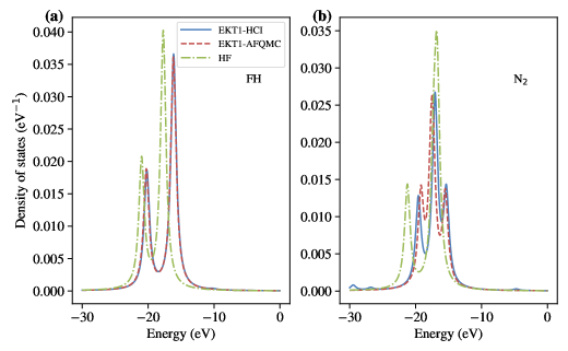
Figure 1: Electron removal spectral functions from various methods (EKT1-HCI, EKT1-AFQMC, and HF) of (a) FH and (b) N2 in the aug-cc-pVDZ basis set. Note that in (a) EKT1-AFQMC is right on top of EKT1-HCI on the plotted scale. A broadening parameter $\eta=0.5$ eV was used.

The main motivation for performing EKT1 within AFQMC was to obtain spectral functions. Poles alone can be obtained using the ground state AFQMC algorithm (i.e., $\Delta$AFQMC) by imposing a proper constraint for excited state descriptions. While the choice of proper trials is a challenge for this purpose, such an approach avoids the complications due to back-propagation. However, spectral weights cannot be obtained from $\Delta$AFQMC. We show EKT1-AFQMC spectral functions for FH and N2 in Fig. 1. Based on the results shown in Table 3, EKT1-AFQMC is in good agreement with EKT1-HCI for FH, but not for N2. Therefore, comparing these two cases is useful for understanding how back-propagation errors are reflected in spectral functions. In the case of FH, we do not see any visible differences between EKT1-HCI and EKT1-AFQMC on the plotted energy scale. However, for N2 we can clearly see some deviation between EKT1-AFQMC and EKT1-HCI. Nonetheless, the main features of the spectral function are reproduced, namely three large quasiparticle peaks with the middle peak being the largest. We note that there are peaks with very small spectral weights in EKT1-HCI close to -30 eV, -27 eV, and -5 eV and that these features these do not appear in EKT1-AFQMC. We attribute this to a relatively large linear dependency cutoff ($10^{-4}$) needed in EKT1-AFQMC to stabilize the generalized eigenvalue problem as explained in Appendix A. In both molecules, there are insignificant differences between the EKT1 and HF spectra in terms of the peak heights, locations and the number of peaks with a brodening parameter of $\eta=0.5$ eV.

IV.2 The uniform electron gas (UEG) model

AFQMC has emerged as a unique tool for simulating correlated solids.Lee et al. (2019a); Zhang et al. (2018); Malone et al. (2020a, b); Lee et al. (2020c) A model solid that describes the basic physics of metallic systems is the UEG model. The accuracy and scope of AFQMC in studying the UEG model has been well documented at zero temperature and finite temperature.Lee et al. (2019a, 2020c) Motivated by these studies, we investigate the spectral properties of the UEG model within the EKT approaches (EKT1 and EKT3).

IV.2.1 14-electrons/19-planewaves

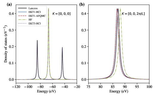
Figure 2: Electron removal spectral functions of the 14-electron in 19-planewave UEG model from various methods at $r_{s}=0.5$: (a) $\mathbf{K}=[0,0,0]$ and (b) $\mathbf{K}=[0,0,2\pi/L]$. In (a), note that EKT1-AFQMC, EKT1-HCI, and HF are right on top of each other. In (b), EKT1-AFQMC and EKT1-HCI are right on top of each other. In both (a) an (b), Lanczos and EKT3-HCI are right on top of each other. A broadening parameter of 0.2 eV was used for all plots.

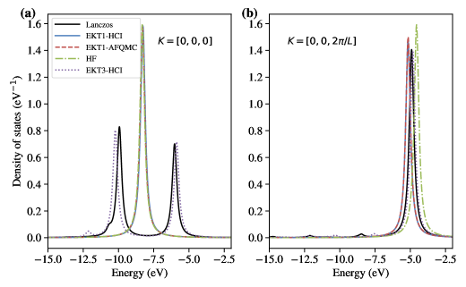
Figure 3: Electron removal spectral functions of the 14-electron in 19-planewave UEG model from various methods at $r_{s}=4.0$: (a) $\mathbf{K}=[0,0,0]$ and (b) $\mathbf{K}=[0,0,2\pi/L]$. In (a), note that EKT1-AFQMC, EKT1-HCI, and HF are right on top of each other. In (b), EKT1-AFQMC and EKT1-HCI are nearly on top of each other. A broadening parameter of 0.2 eV was used for all plots.

The first example that we consider is a relatively small UEG supercell with only 19 planewaves. It is far from the basis set limit as well as from the thermodynamic limit. However, it is small enough for one to produce unbiased EKT results using HCI and numerically exact dynamical Lanczos results. We note that the spectral function of this benchmark UEG model at $r_{s}=4$ was first presented in Ref. 50. We produced around 3000 back-propagation samples, which yielded the largest statistical error in the Fock matrix and 1-RDM on the order of $5\times 10^{-4}$.

We consider two Wigner-Seitz radii, $r_{s}=0.5$ and $r_{s}=4$. Based on our previous benchmark study of AFQMC on this system, we expect that the phaseless error in the ground state at $r_{s}=0.5$ is negligible while the error is relatively more noticeable at $r_{s}=4$.Lee et al. (2019a) Compared to the numerically exact energies, it was found that the constraint bias in AFQMC is only -0.0118(6) eV at $r_{s}=0.5$ and 0.185(2) eV at $r_{s}=4$. Given this small ground state bias, we expect the EKT1-AFQMC approach would be as accurate as EKT1-HCI if good statistics and accuracy in the back-propagated estimators can be achieved.

In Fig. 2, we present spectral functions of this model at $r_{s}=0.5$ for two momenta. The first is at $\mathbf{K}=[0,0,0]$ which represents removal of an electron from the core shell of the UEG model. Core spectra have been shown to have rich satellite features where different many body methods do not agree in terms of the precise satellite structure.McClain et al. (2016) However, such features are very simple in a small supercell like this one. As can be seen in Fig. 2(a), we only have two peaks from the Lanczos method. Neither of these peaks corresponds to a single Koopmans-like excitation. Namely, they cannot be found from a simple single ionization process that either HF (i.e., Koopmans theorem) or EKT1 describes well. As a result of this, HF, EKT1-AFQMC, and EKT-HCI all fail to capture the peak split and only yield a single peak. The correlation effect is very marginal in the sense that nearly no improvement was observed with the EKT1 methods compared to HF.

A significant improvement can be made by incorporating higher-order terms such as 2h1p excitations. In other words, core ionization satellite states (up to leading order) require excitations such as

$$(\sum_{\mathbf{K}^{\prime}\neq\mathbf{0}}C_{\mathbf{K}^{\prime}}\hat{a}^{\dagger}_{\mathbf{K}^{\prime}}\hat{a}_{\mathbf{K}^{\prime}})\hat{a}_{\mathbf{K}=\mathbf{0}}$$ (70)

where $C_{\mathbf{K}^{\prime}}$ are the excitation amplitudes. All of these excitations are included in EKT3. EKT3-HCI can nearly completely reproduce the exact spectral function despite the use of the cumulant approximation for the 4-RDM. The cumulant approximation error is small especially in weakly correlated cases such as $r_{s}=0.5$ where the connected component of 4-RDM is expected to be small. In Fig. 2(b), we emphasize that we observe meaningful improvements even from the EKT1 methods compared to HF. $\mathbf{K}=[0,0,2\pi/L]$ corresponds to the top of the valence band corresponding to the first IP of the UEG model. There is no satellite peak visible at this momentum and the single peak found from the EKT1 methods is reasonable. The peak location of HF is displaced by about +0.9 eV from the correct location while the EKT1 methods yield a peak shifted by about -0.6 eV. We note that EKT1-AFQMC is practically indistinguishable from EKT1-HCI for both momenta which indicates a small phaseless bias, a small back-propagation error, and good statistics for the estimators.

A similar conclusion can be drawn for $r_{s}=4$ as shown in Fig. 3. For the core excitation spectrum in Fig. 3(a), we observe the same split peak structure observed at $r_{s}=0.5$. We see another smaller peak emerging on the left shoulder of the peak near -12 eV. While EKT3-HCI is no longer exact, it reproduces most of the features in the exact spectral function including the emergence of the third peak. While EKT1-HCI and EKT1-AFQMC agree well, there is no visible improvement over HF. The EKT1 methods all yield a single peak which is qualitatively wrong. The valence excitation structure illustrated in Fig. 3(b) is relatively featureless, but there are small peaks emerging in the high energy (more negative) region of the spectrum. EKT3-HCI shows good agreement with Lanczos for the main quasiparticle peak and also produces satellite features. There is a visible improvement of EKT1 approaches (with a deviation of the peak energy of approximately -0.25 eV) compared to HF (with an approximate deviation of +0.34 eV). A slight deviation of EKT1-AFQMC from EKT1-HCI is observed, but the difference in the main quasiparticle peak location is only about 0.01 eV.

Overall, in this small benchmark study, the EKT1 approaches provide some improvement over HF for valence excitations and qualitatively fails for the core region. The agreement between the EKT1 valence peaks and the Lanczos peaks is not perfect, with an error of about -0.6 eV for $r_{s}=0.5$ and -0.25 eV for $r_{s}=4$. However, we emphasize again that we expect EKT1 to become exact for the first IP as the complete basis set limit is approached. Finally, EKT1-AFQMC is able to reproduce EKT1-HCI nearly perfectly even for $r_{s}=4$, where the phaseless error in the ground state energy is about 0.185(2) eV.

IV.2.2 54-electrons/287-planewaves

Next, we consider a larger UEG supercell (54 electrons in 287 planewaves) where obtaining many back-propagation samples is difficult. We study $r_{s}=2$, where AFQMC can be reliably extrapolated to the basis set limit.Lee et al. (2019a) We produced 600 back-propagation samples with a back propagation time of 8 a.u. This amounts to a total of 4800 a.u. propagation time, which is a long propagation for this system size. Our approach yielded a maximum statistical error in 1-RDM and Fock matrices of $4\times 10^{-3}$. While this error is not small, the procedure described in Appendix A was enough to stabilize the final results. Unlike previous cases, we take the upper triangular part of the Fock matrix and explicitly symmetrize the Fock matrix. A linear dependency cutoff of $10^{-3}$ was used in EKT1-AFQMC. It is difficult to generate highly accurate 1- and 2-RDMs from HCI for this system size, so for this system we do not have an exact benchmark reference to compare to our EKT1-AFQMC results. Similarly, EKT3-HCI is also intractable for this system size. Instead, we have performed EOM-IP-CCSD and $\Delta$AFQMC to compare with and to gauge the magnitude of the errors of EKT1-AFQMC.

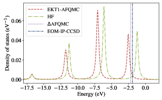
Figure 4: Electron removal spectral functions of the 54-electron in 287-planewave UEG model at $r_{s}=2$ from EKT1-AFQMC and HF. The first IPs from $\Delta$AFQMC and EOM-IP-CCSD are shown for comparisons. A broadening parameter of 0.2 eV was used for all plots.

In Fig. 4, EKT1-AFQMC and HF spectral functions are shown. As expected, EKT1-AFQMC does not show any satellite peaks at all and EKT1-AFQMC only introduces a shift to the HF spectrum. Correlation effects in the peak height do not appear large, but the peak location changes by about 1 eV going from HF to EKT1-AFQMC. We also produced $\Delta$AFQMC and EOM-IP-CCSD for comparison. The $\Delta$AFQMC IP is 2.18(1) eV, EOM-IP-CCSD yields 1.91 eV, and EKT1-AFQMC gives 2.51 eV in this basis set. The deviation of EKT1-AFQMC from $\Delta$AFQMC is 0.33(1) eV whereas EOM-IP-CCSD deviates by 0.27(1) eV. These deviations are similar in magnitude but with opposite signs. The accuracy of EOM-IP-CCSD is unclear because the ground state energy found from CCSD is higher than that of AFQMC by 0.0291(1) eV per electron. In the basis set limit, AFQMC was found to be as accurate as state-of-the-art diffusion Monte Carlo for the ground state energy, differing by 0.0088(9) eV per electron or less.Lee et al. (2019a) This suggests that the ground state correlation energy of CCSD may be on the order of 0.03 eV per electron. How much of this error is propagated to the EOM-IP-CCSD calculation remains unclear. In the complete basis set limit, we believe that the first IP from EKT1-AFQMC will become more accurate and closer to that of $\Delta$AFQMC. A more complete comparison should be conducted in this limit, but such calculations are very difficult due to the need to procure many back-propagation samples in EKT1-AFQMC.

IV.3 Towards ab-initio solids: diamond at the $\Gamma$-point

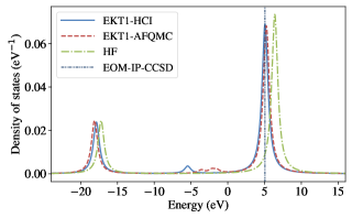
Figure 5: EKT1-HCI and EKT1-AFQMC electron removal spectral functions of diamond at the $\Gamma$-point. A broadening parameter $\eta=0.5$ eV was used.

With recent advances in open-source software such as PySCF,Sun et al. (2018) performing calculations on ab-initio solids is relatively straightforward. While an implementation of AFQMC with $\mathbf{k}$-points has been previously presented,Motta et al. (2019); Malone et al. (2020a) we only present a $\Gamma$-point result in this work. This is mainly because our current EKT1 implementation does not explicitly consider $\mathbf{k}$-points. We chose to study diamond because it is one of the simplest solids just with two carbon atoms in its unit cell. We used the GTH-PADE pseudopotentialGoedecker et al. (1996) and the GTH-DZVP basis set.VandeVondele and Hutter (2007)

This system is overall as small as the smaller systems considered in this work. Therefore, we could obtain over 6000 back-propagation samples with a 4 a.u. back-propagation time. Even with these many samples, the largest error bar in the Fock and 1-RDM matrices was $6\times 10^{-3}$. Due to this large statistical error in the matrix elements, we used a linear dependency cutoff of 0.01 and symmetrized the Fock matrix by taking only the upper triangular part of it (see Appendix A for details). We also included the shift by the Madelung constant in the spectral functions.

As shown in Fig. 5, EKT1-AFQMC successfully reproduces EKT1-HCI. A small quasiparticle peak near -5 eV is not accurately captured by EKT1-AFQMC largely due to statistical noise. Small peaks are difficult to resolve in EKT1-AFQMC without reducing the statistical errors on each matrix element further. Nonetheless, two other larger quasiparticle peaks are well represented. Both peaks are well reproduced within 0.25 eV from EKT1-HCI. The improvement over HF is about 1 eV or so and the first IP from EOM-IP-CCSD is within 0.02 eV of the EKT1-HCI result. It will be interesting to revisit the assessment of EKT1-AFQMC in the basis set and thermodynamic limits via direct comparisons to experiments.

V Conclusions

In this work, we have explored the extended Koopmans’ theorem (EKT) approach to the computation of spectral functions via phaseless auxiliary-field quantum Monte Carlo (AFQMC). Previous attempts in AFQMC to obtaining spectral functions have resorted to analytic continuationMotta et al. (2015); Vitali et al. (2016) which has well-documented drawbacks.Goulko et al. (2017); Dornheim et al. (2018) The EKT approach is attractive because it requires neither an explicit representation of the ground state wavefunction nor analytic continuation to compute spectral functions. Instead, its only inputs are N-particle reduced density matrices (N-RDMs) which can be computed in AFQMC via the back-propagation algorithm. The motivation of our work was thus to use the EKT approach with the aim of avoiding numerical problems arising in analytic continuation for the accurate assessment of real-frequency spectral information. While many studies have so far focused on the simplest level of the EKT, the EKT approach is systematically improvable with increasing order of excitations: 1h, 1p2h, etc. for electron removal and 1p, 1h2p, etc. for electron addition. We presented the implementation of EKT1 (1h or 1p) and EKT3 (1p2h or 1h2p). For EKT3, we proposed the use of a cumulant approximation to the 4-RDM to avoid the steep storage requirements.

We produced preliminary results using EKT1 within AFQMC (EKT1-AFQMC) for small molecular systems, uniform electron gas (UEG) 14-electron and 54-electron supercells, and diamond at the $\Gamma$-point. We focused on studying the first ionization potential (IP) and electron removal spectral functions of these systems. By comparing numerically exact EKT1 results based on heat-bath configuration interaction (i.e., EKT1-HCI), we showed that despite statistical noise, EKT1-AFQMC can capture most qualitative features of EKT1-HCI. We provide a more detailed summary on our findings as follows:

1. In small molecular benchmarks within the aug-cc-pVDZ basis, we found the maximum deviation of EKT1-AFQMC from EKT1-HCI in the first IP to be 0.19 eV. These molecules have quite small phaseless biases in the ground state energy ($\leq 0.04$ eV) so we attributed additional biases to back-propagation. Electron removal spectral functions from EKT1-AFQMC look qualitatively similar to that of EKT1-HCI even in the least accurate case (N2).

2. For the 14-electron UEG supercell (19-planewave) benchmark, we observed a qualitative failure of EKT1 due to its inability to describe satellite states at $\mathbf{K}=\mathbf{0}$. We showed that EKT3 (within HCI) significantly improves this. Despite these failures of EKT1, we found EKT1-AFQMC to have peak locations that are nearly identical (within 0.01 eV) to EKT1-HCI for both $r_{s}=0.5$ and $r_{s}=4$. Given the noticeable phaseless bias at $r_{s}=4$, this result is quite encouraging. Lastly, for the valence region of the electron removal spectral function, we observed reasonable accuracy of EKT1 compared to the exact spectral function. The location of the first IP was off by 0.4 eV for $r_{s}=0.5$ and 0.25 eV for $r_{s}=4.0$, which we expect to improve in larger bases.

3. For the 54-electron UEG supercell (257-planewave) benchmark, we could not obtain EKT1-HCI due computational expense. Therefore, we attempted to assess the accuracy of EKT1-AFQMC by comparing the first IP of EKT1-AFQMC with that of equation-of-motion IP coupled-cluster with singles and doubles (EOM-IP-CCSD) and $\Delta$-AFQMC. However, all three methods differ from each other by more than 0.25 eV and a more thorough benchmark in the basis set limit is highly desirable.

4. For diamond at the $\Gamma$-point, EKT1-AFQMC produced a qualitatively correct electron removal spectral function which agrees well with EKT1-HCI. However, EKT1-AFQMC peak locations were off by 0.2 eV from those of EKT1-HCI. We also noted that EKT1-HCI first IP agrees with that of EOM-IP-CCSD within 0.01 eV.

While a more extensive benchmark study is highly desirable, we cautiously conclude that EKT1-AFQMC is useful for charge excitations that are heavily dominated by Koopmans-like excitations. EKT1-AFQMC errors in peak locations can be as large as 0.25 eV compared to EKT1-HCI, but the line shapes of EKT1-AFQMC closely follow those of EKT1-HCI in all systems considered in this work.

The greatest challenge of EKT1-AFQMC is currently the statistical inefficiency in obtaining relevant back-propagated quantities with error bars small enough to enable the construction of stable EKT1-AFQMC spectral functions. Future work must first be dedicated to improving the statistical efficiency of back-propagation. Furthermore, better back-propagation algorithms are needed to reduce the back-propagation error further. A practical implementation of EKT3-AFQMC using an iterative eigenvalue solver will be an interesting topic to explore in the future. Several interesting extensions are immediately possible. First, extending the EKT framework to neutral excitationsPavlyukh (2018, 2019) is relatively straightforward and could be interesting to explore. Next, the extension of the EKT framework for finite-temperature coupled electron-phonon problems would provide a way to compute temperature-dependent vibronic spectra directly from AFQMC.Lee et al. (2020c, d) We also leave the comparison of these EKT-based spectral functions to analytically continued spectral functions for a future study.

VI Acknowledgements

We thank Sandeep Sharma for providing access to a version of Dice with the 3-RDM and 4-RDM capability which was used in testing and producing EKT3-HCI results presented in this work. We also thank Garnet Chan for discussion about finite-size corrections to ionization energies. DRR acknowledges support of NSF CHE- 1954791. The work of FDM and MAM was performed under the auspices of the U.S. Department of Energy (DOE) by LLNL under Contract No. DE-AC52-07NA27344 and was supported by the U.S. DOE, Office of Science, Basic Energy Sciences, Materials Sciences and Engineering Division, as part of the Computational Materials Sciences Program and Center for Predictive Simulation of Functional Materials (CPSFM). Computing support for this work came from the LLNL Institutional Computing Grand Challenge program.

Appendix A Numerical Details of EKT

Determining the eigenvalues and eigenvectors of Eq. 11 from noisy QMC density matrices is non-trivial. We first diagonalise the metric matrices $S_{\pm}$,

$$S_{\pm}=\mathbf{U}\Lambda_{\pm}\mathbf{U}^{\dagger},$$ (71)

and discard eigenvalues below a given threshold. In this work, unless noted otherwise, in the main text we used $10^{-4}$ for all EKT1-AFQMC results, which is on the order of the largest statistical error in the EKT1 Fock matrix. We next construct the transformation matrix

$$\mathbf{X}_{\pm}=\mathbf{U}\mathbf{\Lambda_{\pm}^{-1/2}}.$$ (72)

This procedure is often referred to as canonical orthogonalization in quantum chemistry. Then, we solve

$$\tilde{\mathbf{F}}_{\pm}\tilde{\mathbf{c}}^{\nu}_{\pm}=\epsilon_{\pm}^{\nu}\tilde{\mathbf{c}}^{\nu}_{\pm},$$ (73)

where

$$\tilde{\mathbf{F}}_{\pm}=\mathbf{X}_{\pm}{{}^{\dagger}}\mathbf{F}_{\pm}\mathbf{X}_{\pm}.$$ (74)

Finally the eigenvectors in the original basis can be determined from

$$(\mathbf{c}^{\nu}_{\pm})_{p}=\sum_{I}(\mathbf{X}_{\pm})_{pI}(\tilde{\mathbf{c}^{\nu}}_{\pm})_{I}.$$ (75)

Following Kent et al.,Kent et al. (1998) we explicitly zero out all matrix elements whose magnitude is smaller than two times the corresponding statistical error bar. We explicitly symmetrize RDMs, but leave the Fock matrix asymmetric as required for approximate wavefunctions. However, for the more difficult problems considered in this work, such as the 54-electron UEG electron and diamond, we found that symmetrizing the Fock matrix is useful so we choose to symmetrize the Fock matrix in such cases (by taking only the upper triangular part of the Fock matrix). These steps improved the numerical stability of the eigenvalue problem.

We also note that there are generic numerical issues arising in EKT even without any statistical sampling error. This was observed in both EKT1-HCI and EKT3-HCI, where spurious solutions with large negative IPs appear. These states stem from the fact that the metric matrix in EKT problems are generally low-rank, as they are related to RDMs. For instance, in the EKT1 formulation, the metric we diagonalize for the IP problem is a 1-RDM whose rank is not so much larger than the number of electrons in the system. These spurious states can be removed with larger cutoffs while often affecting peak locations of quasiparticle states. Interestingly, these spurious states all carry negligible spectral weights and do not appear in spectra. Motivated by this observation, the most satisfying solution we found was to use as a small threshold as possible and to measure the overlap between Koopmans states and eigenvectors to identify quasiparticle-like eigenvectors. This was enough to identify physical IP excitations that are quasi-particle-like. The same principle is applicable to EKT3-HCI and also the EA calculations.

Spectral functions are plotted by approximating the $\delta$-function in the spectral function expression as a Lorentzian function

$$\delta(\omega)\simeq\frac{1}{\pi}\left(\frac{\eta}{\omega^{2}+\eta^{2}}\right)$$ (76)

for some small constant $\eta$. To ensure reproducibility, we specified the value of $\eta$ in all relevant figures.

References

- Lu et al. (2012) D. Lu, I. M. Vishik, M. Yi, Y. Chen, R. G. Moore, and Z.-X. Shen, Annu. Rev. Condens. Matter Phys. 3, 129 (2012).
- Egerton (2008) R. F. Egerton, Rep. Prog. Phys. 72, 016502 (2008).
- Andreani et al. (2005) C. Andreani, D. Colognesi, J. Mayers, G. Reiter, and R. Senesi, Adv. Phys. 54, 377 (2005).
- Fetter and Walecka (2003) A. L. Fetter and J. D. Walecka, Quantum Theory of Many-Particle Systems (Dover Books on Physics) (Dover Publications, 2003).
- Onida et al. (2002) G. Onida, L. Reining, and A. Rubio, Rev. Mod. Phys. 74, 601 (2002).
- Cederbaum and Domcke (1977) L. Cederbaum and W. Domcke, Adv. Chem. Phys 36, 205 (1977).
- Hedin et al. (1998) L. Hedin, J. Michiels, and J. Inglesfield, Phys. Rev. B 58, 15565 (1998).
- Duchemin and Blase (2020) I. Duchemin and X. Blase, J. Chem. Theory Comput. 16, 1742 (2020).
- Hybertsen and Louie (1986) M. S. Hybertsen and S. G. Louie, Phys. Rev. B 34, 5390 (1986).
- Hedin (1965) L. Hedin, Phys. Rev. 139, A796 (1965).
- Reining (2018) L. Reining, Wiley Interdiscip. Rev. Comput. Mol. Sci. 8, e1344 (2018).
- Rinke et al. (2005) P. Rinke, A. Qteish, J. Neugebauer, C. Freysoldt, and M. Scheffler, New J. Phys. 7, 126 (2005).
- Fuchs et al. (2007) F. Fuchs, J. Furthmüller, F. Bechstedt, M. Shishkin, and G. Kresse, Phys. Rev. B 76, 115109 (2007).
- Marom et al. (2012) N. Marom, F. Caruso, X. Ren, O. T. Hofmann, T. Körzdörfer, J. R. Chelikowsky, A. Rubio, M. Scheffler, and P. Rinke, Phys. Rev. B 86, 245127 (2012).
- Bruneval (2012) F. Bruneval, J. Chem. Phys. 136, 194107 (2012).
- Langreth (1970) D. C. Langreth, Phys. Rev. B 1, 471 (1970).
- Aryasetiawan et al. (1996) F. Aryasetiawan, L. Hedin, and K. Karlsson, Phys. Rev. Lett. 77, 2268 (1996).
- Guzzo et al. (2011) M. Guzzo, G. Lani, F. Sottile, P. Romaniello, M. Gatti, J. J. Kas, J. J. Rehr, M. G. Silly, F. Sirotti, and L. Reining, Phys. Rev. Lett. 107, 166401 (2011).
- Lischner et al. (2013) J. Lischner, D. Vigil-Fowler, and S. G. Louie, Phys. Rev. Lett. 110, 146801 (2013).
- Stan et al. (2009) A. Stan, N. E. Dahlen, and R. Van Leeuwen, J. Chem. Phys. 130, 114105 (2009).
- von Barth and Holm (1996) U. von Barth and B. Holm, Phys. Rev. B 54, 8411 (1996).
- Holm and von Barth (1998) B. Holm and U. von Barth, Phys. Rev. B 57, 2108 (1998).
- Faleev et al. (2004) S. V. Faleev, M. Van Schilfgaarde, and T. Kotani, Phys. Rev. Lett. 93, 126406 (2004).
- van Schilfgaarde et al. (2006) M. van Schilfgaarde, T. Kotani, and S. Faleev, Phys. Rev. Lett. 96, 226402 (2006).
- Shishkin and Kresse (2007) M. Shishkin and G. Kresse, Phys. Rev. B 75, 235102 (2007).
- Rostgaard et al. (2010) C. Rostgaard, K. W. Jacobsen, and K. S. Thygesen, Phys. Rev. B 81, 085103 (2010).
- Koval et al. (2014) P. Koval, D. Foerster, and D. Sánchez-Portal, Phys. Rev. B 89, 155417 (2014).
- Bobbert and Van Haeringen (1994) P. Bobbert and W. Van Haeringen, Phys. Rev. B 49, 10326 (1994).
- Schindlmayr and Godby (1998) A. Schindlmayr and R. W. Godby, Phys. Rev. Lett. 80, 1702 (1998).
- Romaniello et al. (2009) P. Romaniello, S. Guyot, and L. Reining, J. Chem. Phys. 131, 154111 (2009).
- Chen and Pasquarello (2015) W. Chen and A. Pasquarello, Phys. Rev. B 92, 041115 (2015).
- Maggio and Kresse (2017) E. Maggio and G. Kresse, J. Chem. Theory Comput. 13, 4765 (2017).
- Holm and Aryasetiawan (1997) B. Holm and F. Aryasetiawan, Phys. Rev. B 56, 12825 (1997).
- Kas et al. (2014) J. J. Kas, J. J. Rehr, and L. Reining, Phys. Rev. B 90, 085112 (2014).
- Lischner et al. (2014) J. Lischner, D. Vigil-Fowler, and S. G. Louie, Phys. Rev. B 89, 125430 (2014).
- Caruso and Giustino (2016) F. Caruso and F. Giustino, Eur. Phys. J. B 89 (2016).
- Mayers et al. (2016) M. Z. Mayers, M. S. Hybertsen, and D. R. Reichman, Phys. Rev. B 94, 081109 (2016).
- Jeckelmann (2002) E. Jeckelmann, Phys. Rev. B 66, 045114 (2002).
- Schollwöck and White (2006) U. Schollwöck and S. R. White, AIP Conf. Proc. 816, 155 (2006).
- Schirmer (1982) J. Schirmer, Phys. Rev. A 26, 2395 (1982).
- Schirmer et al. (1983) J. Schirmer, L. S. Cederbaum, and O. Walter, Phys. Rev. A 28, 1237 (1983).
- Tarantelli and Cederbaum (1989) A. Tarantelli and L. S. Cederbaum, Phys. Rev. A 39, 1656 (1989).
- Wenzel et al. (2014) J. Wenzel, M. Wormit, and A. Dreuw, J. Chem. Theory Comput. 10, 4583 (2014).
- Dreuw and Wormit (2015) A. Dreuw and M. Wormit, WIREs Comput. Mol. Sci. 5, 82 (2015).
- Sokolov (2018) A. Yu. Sokolov, J. Chem. Phys. 149, 204113 (2018).
- Monkhorst (1977) H. J. Monkhorst, Int. J. Quantum Chem. 12, 421 (1977).
- Nooijen and Snijders (1992) M. Nooijen and J. G. Snijders, Int. J. Quantum Chem. 44, 55 (1992).
- Nooijen and Snijders (1993) M. Nooijen and J. G. Snijders, Int. J. Quantum Chem. 48, 15 (1993).
- Peng and Kowalski (2016) B. Peng and K. Kowalski, Phys. Rev. A 94, 062512 (2016).
- McClain et al. (2016) J. McClain, J. Lischner, T. Watson, D. A. Matthews, E. Ronca, S. G. Louie, T. C. Berkelbach, and G. K.-L. Chan, Phys. Rev. B 93, 235139 (2016).
- McClain et al. (2017) J. McClain, Q. Sun, G. K.-L. Chan, and T. C. Berkelbach, J. Chem. Theory Comput. 13, 1209 (2017).
- Furukawa et al. (2018) Y. Furukawa, T. Kosugi, H. Nishi, and Y.-i. Matsushita, J. Chem. Phys. 148, 204109 (2018).
- Peng and Kowalski (2018) B. Peng and K. Kowalski, Mol. Phys. 116, 561 (2018).
- Shee and Zgid (2019) A. Shee and D. Zgid, J. Chem. Theory Comput. 15, 6010 (2019).
- Blankenbecler and Sugar (1983) R. Blankenbecler and R. L. Sugar, Phys. Rev. D 27, 1304 (1983).
- Becca and Sorella (2017) F. Becca and S. Sorella, Quantum Monte Carlo Approaches for Correlated Systems (Cambridge University Press, Cambridge, England, UK, 2017).
- Foulkes et al. (2001) W. M. C. Foulkes, L. Mitas, R. J. Needs, and G. Rajagopal, Rev. Mod. Phys. 73, 33 (2001).
- Silver et al. (1990) R. N. Silver, D. S. Sivia, and J. E. Gubernatis, Phys. Rev. B 41, 2380 (1990).
- Gubernatis et al. (1991) J. E. Gubernatis, M. Jarrell, R. N. Silver, and D. S. Sivia, Phys. Rev. B 44, 6011 (1991).
- Jarrell and Gubernatis (1996) M. Jarrell and J. E. Gubernatis, Phys. Rep. 269, 133 (1996).
- Motta et al. (2014) M. Motta, D. E. Galli, S. Moroni, and E. Vitali, J. Chem. Phys. 140, 024107 (2014).
- Motta et al. (2015) M. Motta, D. E. Galli, S. Moroni, and E. Vitali, J. Chem. Phys. 143, 164108 (2015).
- Otsuki et al. (2017) J. Otsuki, M. Ohzeki, H. Shinaoka, and K. Yoshimi, Phys. Rev. E 95, 061302 (2017).
- Bertaina et al. (2017) G. Bertaina, D. E. Galli, and E. Vitali, Adv. Phys-X 2, 302 (2017).
- Reichman and Rabani (2009) D. R. Reichman and E. Rabani, J. Chem. Phys. 131, 054502 (2009).
- Goulko et al. (2017) O. Goulko, A. S. Mishchenko, L. Pollet, N. Prokof’ev, and B. Svistunov, Phys. Rev. B 95, 014102 (2017).
- Dornheim et al. (2018) T. Dornheim, S. Groth, J. Vorberger, and M. Bonitz, Phys. Rev. Lett. 121, 255001 (2018).
- Ceperley and Bernu (1988) D. M. Ceperley and B. Bernu, J. Chem. Phys. 89, 6316 (1988).
- Blunt et al. (2015) N. S. Blunt, A. Alavi, and G. H. Booth, Phys. Rev. Lett. 115, 050603 (2015).
- Blunt et al. (2018) N. S. Blunt, A. Alavi, and G. H. Booth, Phys. Rev. B 98, 085118 (2018).
- Booth et al. (2009) G. H. Booth, A. J. W. Thom, and A. Alavi, J. Chem. Phys. 131, 054106 (2009).
- Day et al. (1975) O. W. Day, D. W. Smith, and R. C. Morrison, J. Chem. Phys. 62, 115 (1975).
- Smith and Day (1975) D. W. Smith and O. W. Day, J. Chem. Phys. 62, 113 (1975).
- Pickup (1975) B. T. Pickup, Chem. Phys. Lett. 33, 422 (1975).
- Morrison et al. (1975) R. C. Morrison, O. W. Day, and D. W. Smith, Int. J. Quantum Chem. 9, 229 (1975).
- Ellenbogen et al. (1977) J. C. Ellenbogen, O. W. Day, D. W. Smith, and R. C. Morrison, J. Chem. Phys. 66, 4795 (1977).
- Morrison and Liu (1992) R. C. Morrison and G. Liu, J. Comp. Chem. 13, 1004 (1992).
- Morrison (1992) R. C. Morrison, J. Chem. Phys. 96, 3718 (1992).
- Sundholm and Olsen (1993) D. Sundholm and J. Olsen, J. Chem. Phys. 98, 3999 (1993).
- Cioslowski et al. (1997) J. Cioslowski, P. Piskorz, and G. Liu, J. Chem. Phys. 107, 6804 (1997).
- Kent et al. (1998) P. Kent, R. Q. Hood, M. Towler, R. Needs, and G. Rajagopal, Phys. Rev. B - Condensed Matter and Materials Physics 57, 15293 (1998).
- Olsen and Sundholm (1998) J. Olsen and D. Sundholm, Chem. Phys. Lett. 288, 282 (1998).
- Pernal and Cioslowski (2001) K. Pernal and J. Cioslowski, J. Chem. Phys. 114, 4359 (2001).
- Farnum and Mazziotti (2004) J. D. Farnum and D. A. Mazziotti, Chem. Phys. Lett. 400, 90 (2004).
- Pernal and Cioslowski (2005) K. Pernal and J. Cioslowski, Chem. Phys. Lett. 412, 71 (2005).
- Ernzerhof (2009) M. Ernzerhof, J. Chem. Theory Comput. 5, 793 (2009).
- Vanfleteren et al. (2009) D. Vanfleteren, D. Van Neck, P. W. Ayers, R. C. Morrison, and P. Bultinck, J. Chem. Phys. 130 (2009), 10.1063/1.3130044.
- Piris et al. (2012) M. Piris, J. M. Matxain, X. Lopez, and J. M. Ugalde, J. Chem. Phys. 136, 174116 (2012).
- Piris et al. (2013) M. Piris, J. M. Matxain, X. Lopez, and J. M. Ugalde, in 8th Congress on Electronic Structure: Principles and Applications (ESPA 2012): A Conference Selection from Theoretical Chemistry Accounts (Springer, Berlin, Germany, 2013) pp. 5–15.
- Bozkaya (2013) U. Bozkaya, J. Chem. Phys. 139 (2013), 10.1063/1.4825041.
- Welden et al. (2015) A. R. Welden, J. J. Phillips, and D. Zgid, , 1 (2015), arXiv:1505.05575 .
- Bozkaya and Ünal (2018) U. Bozkaya and A. Ünal, J. Phys. Chem. A 122, 4375 (2018).
- Pavlyukh (2018) Y. Pavlyukh, Phys. Rev. A 98, 1 (2018).
- Pavlyukh (2019) Y. Pavlyukh, Phys. Status Solidi B Basic Res. 256, 1 (2019).
- Zheng (2016) H. Zheng, “First principles quantum Monte Carlo study of correlated electronic systems,” (2016), [Online; accessed 12. Jan. 2021].
- Zhang et al. (1995) S. Zhang, J. Carlson, and J. E. Gubernatis, Phys. Rev. Lett. 74, 3652 (1995).
- Zhang et al. (1997) S. Zhang, J. Carlson, and J. E. Gubernatis, Phys. Rev. B 55, 7464 (1997).
- Zhang and Krakauer (2003) S. Zhang and H. Krakauer, Phys. Rev. Lett. 90, 136401 (2003).
- Carlson et al. (1999) J. Carlson, J. Gubernatis, G. Ortiz, and S. Zhang, Phys. Rev. B 59, 12788 (1999).
- LeBlanc et al. (2015) J. P. LeBlanc, A. E. Antipov, F. Becca, I. W. Bulik, G. K.-L. Chan, C.-M. Chung, Y. Deng, M. Ferrero, T. M. Henderson, C. A. Jiménez-Hoyos, et al., Phys. Rev. X 5, 041041 (2015).
- Zheng et al. (2017) B.-X. Zheng, C.-M. Chung, P. Corboz, G. Ehlers, M.-P. Qin, R. M. Noack, H. Shi, S. R. White, S. Zhang, and G. K.-L. Chan, Science 358, 1155 (2017).
- Motta et al. (2017) M. Motta, D. M. Ceperley, G. K.-L. Chan, J. A. Gomez, E. Gull, S. Guo, C. A. Jiménez-Hoyos, T. N. Lan, J. Li, F. Ma, et al., Phys. Rev. X 7, 031059 (2017).
- Zhang et al. (2018) S. Zhang, F. D. Malone, and M. A. Morales, J. Chem. Phys. 149, 164102 (2018).
- Motta et al. (2020) M. Motta, C. Genovese, F. Ma, Z.-H. Cui, R. Sawaya, G. K.-L. Chan, N. Chepiga, P. Helms, C. Jiménez-Hoyos, A. J. Millis, et al., Phys. Rev. X 10, 031058 (2020).
- Lee et al. (2019a) J. Lee, F. D. Malone, and M. A. Morales, J. Chem. Phys. 151, 064122 (2019a).
- Lee et al. (2020a) J. Lee, F. D. Malone, and D. R. Reichman, J. Chem. Phys. 153, 126101 (2020a).
- Williams et al. (2020) K. T. Williams, Y. Yao, J. Li, L. Chen, H. Shi, M. Motta, C. Niu, U. Ray, S. Guo, R. J. Anderson, et al., Phys. Rev. X 10, 011041 (2020).
- Malone et al. (2020a) F. D. Malone, S. Zhang, and M. A. Morales, J. Chem. Theory Comput. 16, 4286 (2020a).
- Lee et al. (2020b) J. Lee, F. D. Malone, and M. A. Morales, J. Chem. Theory Comput. 16, 3019 (2020b).
- Qin et al. (2020) M. Qin, C.-M. Chung, H. Shi, E. Vitali, C. Hubig, U. Schollwöck, S. R. White, S. Zhang, et al., Phys. Rev. X 10, 031016 (2020).
- Malone et al. (2020b) F. D. Malone, A. Benali, M. A. Morales, M. Caffarel, P. R. C. Kent, and L. Shulenburger, Phys. Rev. B 102, 161104 (2020b).
- Malone et al. (2019) F. D. Malone, S. Zhang, and M. A. Morales, J. Chem. Theory. Comput. 15, 256 (2019).
- Lee and Reichman (2020) J. Lee and D. R. Reichman, J. Chem. Phys. 153, 044131 (2020).
- Purwanto and Zhang (2004) W. Purwanto and S. Zhang, Phys. Rev. E 70, 056702 (2004).
- Motta and Zhang (2017) M. Motta and S. Zhang, J. Chem. Theory Comput. 13, 5367 (2017).
- Hedin (1980) L. Hedin, Phys. Scr. 21, 477 (1980).
- (117) See https://github.com/msaitow/SecondQuantizationAlgebra for details on how to obtain the source code.
- Neuscamman et al. (2009) E. Neuscamman, T. Yanai, and G. K.-L. Chan, J. Chem. Phys. 130, 124102 (2009).
- Saitow et al. (2013) M. Saitow, Y. Kurashige, and T. Yanai, J. Chem. Phys. 139, 044118 (2013).
- Zgid et al. (2009) D. Zgid, D. Ghosh, E. Neuscamman, and G. K.-L. Chan, J. Chem. Phys. 130, 194107 (2009).
- Motta and Zhang (2018) M. Motta and S. Zhang, WIREs Comput. Mol. Sci. 8, e1364 (2018).
- Hubbard (1959) J. Hubbard, Phys. Rev. Lett. 3, 77 (1959).
- Hirsch (1983) J. E. Hirsch, Phys. Rev. B 28, 4059 (1983).
- (124) Mario Motta, private communication.
- Chen et al. (2020) S. Chen, M. Motta, F. Ma, and S. Zhang, arXiv preprint arXiv:2011.08335 (2020).
- Hohenstein et al. (2012a) E. G. Hohenstein, R. M. Parrish, and T. J. Martínez, J. Chem. Phys. 137, 044103 (2012a).
- Parrish et al. (2012) R. M. Parrish, E. G. Hohenstein, T. J. Martínez, and C. D. Sherrill, J. Chem. Phys. 137, 224106 (2012).
- Hohenstein et al. (2012b) E. G. Hohenstein, R. M. Parrish, C. D. Sherrill, and T. J. Martínez, J. Chem. Phys. 137, 221101 (2012b).
- Lee et al. (2019b) J. Lee, L. Lin, and M. Head-Gordon, J. Chem. Theory Comput. 16, 243 (2019b).
- Schoof et al. (2015) T. Schoof, S. Groth, J. Vorberger, and M. Bonitz, Phys. Rev. Lett. 115, 130402 (2015).
- Yang et al. (2020) Y. Yang, V. Gorelov, C. Pierleoni, D. M. Ceperley, and M. Holzmann, Phys. Rev. B 101, 085115 (2020).
- Sun et al. (2018) Q. Sun, T. C. Berkelbach, N. S. Blunt, G. H. Booth, S. Guo, Z. Li, J. Liu, J. D. McClain, E. R. Sayfutyarova, S. Sharma, S. Wouters, and G. K.-L. Chan, WIREs Comput. Mol. Sci. 8, e1340 (2018).
- Kent et al. (2020) P. R. C. Kent, A. Annaberdiyev, A. Benali, M. C. Bennett, E. J. Landinez Borda, P. Doak, H. Hao, K. D. Jordan, J. T. Krogel, I. Kylänpää, J. Lee, Y. Luo, F. D. Malone, C. A. Melton, L. Mitas, M. A. Morales, E. Neuscamman, F. A. Reboredo, B. Rubenstein, K. Saritas, S. Upadhyay, G. Wang, S. Zhang, and L. Zhao, J. Chem. Phys. 152, 174105 (2020).
- (134) See https://github.com/pauxy-qmc/pauxy for details on how to obtain the source code.
- Holmes et al. (2016) A. A. Holmes, N. M. Tubman, and C. J. Umrigar, J. Chem. Theory Comput. 12, 3674 (2016).
- Sharma et al. (2017) S. Sharma, A. A. Holmes, G. Jeanmairet, A. Alavi, and C. J. Umrigar, J. Chem. Theory Comput. 13, 1595 (2017).
- Smith et al. (2017) J. E. T. Smith, B. Mussard, A. A. Holmes, and S. Sharma, J. Chem. Theory Comput. 13, 5468 (2017).
- Wagner et al. (2009) L. K. Wagner, M. Bajdich, and L. Mitas, J. Comput. Phys. 228, 3390 (2009).
- Haydock et al. (1975) R. Haydock, V. Heine, and M. J. Kelly, J. Phys. C: Solid State Phys. 8, 2591 (1975).
- Dagotto (1994) E. Dagotto, Rev. Mod. Phys. 66, 763 (1994).
- van Setten et al. (2015) M. J. van Setten, F. Caruso, S. Sharifzadeh, X. Ren, M. Scheffler, F. Liu, J. Lischner, L. Lin, J. R. Deslippe, S. G. Louie, C. Yang, F. Weigend, J. B. Neaton, F. Evers, and P. Rinke, J. Chem. Theory Comput. 11, 5665 (2015).
- Dunning (1989) T. H. Dunning, J. Chem. Phys. 90, 1007 (1989).
- Lee et al. (2020c) J. Lee, M. A. Morales, and F. D. Malone, arXiv (2020c), 2012.12228 .
- Motta et al. (2019) M. Motta, S. Zhang, and G. K.-L. Chan, Phys. Rev. B 100, 045127 (2019).
- Goedecker et al. (1996) S. Goedecker, M. Teter, and J. Hutter, Phys. Rev. B 54, 1703 (1996).
- VandeVondele and Hutter (2007) J. VandeVondele and J. Hutter, J. Chem. Phys. 127, 114105 (2007).
- Vitali et al. (2016) E. Vitali, H. Shi, M. Qin, and S. Zhang, Phys. Rev. B 94, 085140 (2016).
- Lee et al. (2020d) J. Lee, S. Zhang, and D. R. Reichman, arXiv (2020d), 2012.13473 .