Object Detection Made Simpler by Eliminating Heuristic NMS

Abstract

We show a simple NMS-free, end-to-end object detection framework, of which the network is a minimal modification to a one-stage object detector such as the FCOS detection model [24]. We attain on par or even improved detection accuracy compared with the original one-stage detector. It performs detection at almost the same inference speed, while being even simpler in that now the post-processing NMS (non-maximum suppression) is eliminated during inference. If the network is capable of identifying only one positive sample for prediction for each ground-truth object instance in an image, then NMS would become unnecessary. This is made possible by attaching a compact PSS head for automatic selection of the single positive sample for each instance (see Fig. LABEL:fig:model). As the learning objective involves both one-to-many and one-to-one label assignments, there is a conflict in the labels of some training examples, making the learning challenging. We show that by employing a stop-gradient operation, we can successfully tackle this issue and train the detector.

On the COCO dataset, our simple design achieves superior performance compared to both the FCOS baseline detector with NMS post-processing and the recent end-to-end NMS-free detectors. Our extensive ablation studies justify the rationale of the design choices.

Code is available at: https://git.io/PSS

1 Introduction

Object detection is a fundamental task in computer vision and has been progressed dramatically in the past few years using deep learning. It aims at predicting a set of bounding boxes and the corresponding categories in an image. Modern object detection methods fall into two categories: two-stage detectors, exemplified by Faster R-CNN [19], and one-stage detectors such as YOLO [18], SSD [15], RetinaNet [13]. Recently one-stage detectors become more and more popular due to its simplicity and high performance. Since anchor-free detectors such as FCOS [24] and FoveaBox [10] were introduced, the community tend to recognize that anchor boxes may not be an indispensable design choice for object detection, thus leaving NMS (non maximum suppression) the only heuristic post-processing in the entire pipeline.

The NMS operation has almost always been used in mainstream object detectors in the literature. The necessity of NMS in detection is because one ground-truth object always has multiple positive samples during the course of training. For instance, in [24, 10], all the locations on the CNN feature maps within the center region of an object are assigned positive labels. As a result, multiple network outputs correspond to one target object. The consequence is that for inference, a mechanism (namely, NMS) is needed to choose the best positive sample among all the positive boxes.

Very recently, some methods [1, 34] formulate detection into a set-to-set prediction problem and leverage the Hungarian matching algorithm to tackle the issue of finding one positive sample for each ground-truth box. With the Hungarian matching algorithm, for a ground-truth object, the models adaptively choose the network outputs with minimal loss as the positive sample for the object, while other samples are considered negative. Thus NMS can be removed and the detector becomes end-to-end trainable. Wang et al. [26] design a fully convolutional network (FCN) without using Transformers and achieve end-to-end NMS-free object detection. Our work here follows this avenue by designing even simpler FCN detectors with stronger detection accuracy.

Concretely, in this work we want to design a simple high-performance fully convolutional network for object detection, which is NMS free and fully end-to-end trainable. We instantiate such a design on top of the FCOS detector [24] with minimal modification to the network itself, as shown in Fig. LABEL:fig:model. Indeed, the only modification to FCOS is that i.) a compact “positive sample selector (PSS)” head is introduced, in order to select the optimal positive sample for each object instance; ii.) the learning objective is re-designed to successfully train the detector.

For training the network, we keep the original FCOS classification loss, which is important as it provides rich supervision that encodes desirable invariance encoding. As discussed in §3.4, the label discrepancy between one-to-many and one-to-one label assignments causes the network training challenging. Here, we propose a simple asymmetric optimization scheme: we introduce the stop-grad operation (see Fig. LABEL:fig:model) to stop the gradient relevant to the attached PSS head passing to the original FCOS network parameters.

We empirically show the effectiveness of the stop-grad operation (Fig. 2). This stop-grad can be particularly useful in the following case. The network contains two sub-networks A and B. The optimization of B relies on the convergence of A while the optimization of A does not rely much on B, thus being asymmetric.

Our method does not rely attention mechanisms such as Transformers, or cross-level feature aggregation such as the 3D max filtering [26]. Our proposed detector, termed FCOS_PSS, enjoys the following advantages.

• Detection is now made even simpler by eliminating NMS. With the simplicity inherited from FCOS, FCOS_PSS is fully compatible with other FCN-solvable tasks.

• We show that NMS can be eliminated by introducing a single compact PSS head, with negligible computation overhead compared to the vanilla FCOS.

• The proposed PSS is flexible in that, in essence the PSS head serves as learnable NMS. Because by design we keep the vanilla FCOS heads working as well as the original detector, FCOS_PSS offers flexibility in terms of the NMS being used. For example, once trained, one may choose to discard the PSS head and use FCOS_PSS as the standard FCOS.

• We report on par or even improved detection results on the COCO dataset compared with the standard FCOS [24] and ATSS [32] detectors, as well as recent NMS-free detection methods.

• The proposed PSS head is also applicable to other anchor-box based detectors such as RetinaNet. We achieve promising results by attaching PSS to the modified RetinaNet detector, which uses one square anchor box per location and employs adaptive training sample selection as for improved detection accuracy as in [32].

• The same idea may be applied to some other instance recognition tasks. For example, as we shown in §4.4, we can eliminate NMS from instance segmentation frameworks, e.g., [27, 28]. We wish that the work presented here can benefit those works built upon the FCOS detector including instance segmentation [2, 23, 31, 29], keypoint detection [22], text spotting [16], and tracking [6].

2 Related Work

Object detection has been extensively studied in computer vision as it enables a wide range of downstream applications. Traditional methods use hand-crafted features (e.g., HoG, SIFT) to solve detection as classification on a set of candidate bounding boxes. With the development of deep neural networks, modern object detection methods can be divided into three categories: two-stage detectors, one-stage detectors, and recent end-to-end detectors.

Two-stage Object Detector One line of research focuses on two-stage object detectors such as Faster R-CNN [19], which first generate region proposals, and then refine the detection for each proposal. Mask R-CNN [7] adds a mask prediction branch on top of Faster R-CNN, which can be used to solve a few instance-level recognition tasks, including instance segmentation and pose estimation.

While two-stage detectors still find many applications, the community have been shifting the research focus to one-stage detectors due to its much simpler and cleaner design, with strong performance.

One-stage Object Detector The second line of research develops efficient single-stage object detectors [15, 18, 24, 10], which directly make dense predictions based on extracted feature maps and dense anchors or points. They are based essentially sliding windows. Anchor-based detectors, e.g., YOLO [18] and SSD [15] use a set of pre-defined anchor boxes to predict object category and anchor box offsets. Note that anchors were first proposed in the RPN module of Faster R-CNN to generate proposals.

In one-stage object detection, negative samples are inevitably many more than positive samples, leading to data imbalance training. Techniques such as hard negative mining and the focal loss function [13] were thus proffered to alleviate the imbalance training issue.

Recently, efforts have been spent on designing anchor-free detectors [24, 10]. FCOS [24] and Foveabox [10] use the center region of targets as positive samples. In addition, FCOS introduces the so-called center-ness score to make NMS more accurate. Authors of [32] propose an adaptive training sample selection (ATSS) scheme to automatically define positive and negative training samples, albeit still using a heuristically designed rule. PAA [9] designs a probabilistic anchor assignment strategy, leading to easier training compared to those heuristic IoU hard label assignment strategies. Besides improving the assignment strategy of FCOS [32, 9], efforts were also spent on the detection features [17], loss functions [11] to further boost the anchor-free detector’s performance.

Nevertheless, both the one-stage and two-stage object detectors require a post-processing procedure, namely, non-maximum suppression (NMS), to merge the duplicate detections. That is, most state-of-the-art detectors are not end-to-end trainable.

End-to-end Object Detector Recently, a few works propose end-to-end frameworks for object detection by removing NMS from the pipeline. One of the pioneering works may be attributed to [20]. There, object detection was formulated as a sequence-to-sequence learning task and LSTM-RNN was used to implement the idea. DETR [1] introduces the Transformer-based attention mechanism to object detection. Essentially the sequence-to-sequence learning task in [20] was now solved in parallel by self-attention based Transformer rather than RNN. Deformable DETR [34] accelerates the training convergence of DETR by proposing to only perform attention to a small set of key sampling points.

Very recently, DeFCN [26] adopts a one-to-one matching strategy to enable end-to-end object detection based on a fully convolutional network with competitive performance. Significantly, probably for the first time, DeFCN [26] demonstrates that it is possible to remove NMS from a detector without resorting to sequence-to-sequence (or set-to-set) learning that relies on LSTM-RNN or self-attention mechanisms. The work in [21] shares similarities with DeFCN [26] in the one-to-one label assignment and using auxiliary heads to help training. The performance reported in [21] is inferior to that of DeFCN [26].

We have drawn inspiration from [26] in terms of designing the one-to-one label assignment strategy, as in Equ. (3). Clearly, this one-to-one label assignment has a direct impact on the final NMS-free detection accuracy. One of the main differences is that we use a simple binary classification head to enable selection of one positive sample for each instance, while DeFCN designs 3D max filtering for this purpose, which aggregates multi-scale features to suppress duplicated detections. Second, As mentioned earlier, we have aimed to keep the original FCOS detector intact as much as possible. Next, we present the proposed FCOS_PSS.

3 Our Method

Backbone	Model	mAP (%)	mAR (%)	Network forward (ms)	Post process.  (ms)
R50	FCOS [24]	42.0	60.2	38.76	2.91
	ATSS [32]	42.8	61.4	38.31	7.56
	DeFCN [26]	41.5	61.4
	FCOSPSS (Ours)	42.3	61.6	42.37	1.49
	ATSSPSS (Ours)	42.6	62.1	42.19	3.89
R101	FCOS [24]	43.5	61.3	51.55	3.40
	ATSS[32]	44.2	61.9	51.81	8.80
	FCOSPSS (Ours)	44.1	62.7	54.95	2.52
	ATSSPSS (Ours)	44.2	63.2	55.65	4.32
X-101-DCN	ATSSPSS (Ours)	47.5	65.1	82.64	4.31
R2N-101-DCN	ATSSPSS (Ours)	48.5	66.4	81.30	4.17

Table 1: Performance comparison between our proposed NMS-free detectors and various one-stage detection methods on the COCO val.  set. All the models are trained with the ‘3$\times$’ schedule and multi-scale data augmentation (but with single-scale testing). Here ‘ATSS’ is the modified RetinaNet detector using one square anchor box per location, employing ATSS (adaptive training sample selection) as in [32]. Inference time measures network forward computation and post-processing time (ranking detected boxes to compute mAP for our methods and NMS for others) on a single V100 GPU. Backbones: ‘R’: ResNet [8]. ‘X’: ResNeXt (32$\times$4d-101) [30]. ‘DCN’: Deformable Convolution Network [33]. ‘R2N’: Res2Net [5].

The overall network structure of FCOS_PSS is very straightforward as shown in Fig. LABEL:fig:model. The only modification is the PSS head which has two extra conv. layers, and all the other parts are the same as that of FCOS [24]. We start by presenting the overall training objectives.

3.1 Overall Training Objective

Our overall training targets can be formulated as follows.

$${\cal L}={\cal L}_{fcos}+\lambda_{1}\cdot{\cal L}_{pss}+\lambda_{2}\cdot{\cal L}_{rank}.$$ (1)

Here $\lambda_{1}$, $\lambda_{2}$ are balancing coefficients. ${\cal L}_{fcos}$ contains the loss terms that are exactly same as in the original FCOS [24], namely, $C$-way classification using the focal loss ($C=80$ for the COCO dataset), bounding box regression with the GIoU loss, and the center-ness loss.

We have set $\lambda_{2}$ to $0.25$ in all the experiments as the ranking loss is not essential. As reported in Table 9, the ranking loss improves the final detection accuracy slightly (0.2$\scriptstyle\sim$0.3 points in mAP). We include it here as it does not introduce much training complexity.

3.1.1 PSS Loss ${\cal L}_{pss}$

${\cal L}_{pss}$ is the key to the success of our framework, which is a classification loss associated to the positive sample selector. Recall that our goal is to select one and only one positive sample for each instance in an image. Here the newly added PSS head is expected to achieve this goal. We defer the details of one-to-one positive label assignment to §3.3 and let us assume that the one optimal ground-truth positive label for each instance is available. As shown in Fig. LABEL:fig:model, the output of the PSS head is a map of ${\mathbb{R}}^{H\times W\times 1}$. Let us denote $\sigma({\rm pss})$ a single point of this map. Then the learning target for $\sigma({\rm pss})$ is $1$ if it corresponds to the positive sample of an instance; otherwise negative labels. Thus, the simplest approach would be to train a binary classifier. Here, in order to take advantage of the $C$-way classifier in FCOS, we again formulate the loss term as $C$-way classification.

Specifically, the loss term calculates the focal loss between the multiplied score of:

$$\sigma({\rm pss})\cdot\sigma(s)\cdot\sigma({\rm ctr})$$

against the ground-truth labels of $C$ categories, with $\sigma(s)$ being the score map of the FCOS classifier’s output. Note that, the difference between this classifier and the vanilla FCOS’ classifier is that here we now have only one positive sample for each object instance in an image. After learning, ideally, $\sigma({\rm pss})$ is able to activate one and only one positive sample for an object instance.

3.1.2 Ranking Loss ${\cal L}_{rank}$

Our pilot experiment show that including a ranking loss term in the objective function can help improve the performance of our NMS-free detectors. Specifically, we add the ranking loss of Equ. (2) for each training image:

$${\cal L}_{rank}=\frac{1}{n_{-}n_{+}}\sum_{i_{-}}^{n_{-}}\sum_{i_{+}}^{n_{{}_{+}}}\text{max}(0,\gamma-\hat{P}_{i_{+}}(c_{i_{+}})+\hat{P}_{i_{-}}(c_{i_{-}}))$$ (2)

Here, $\gamma$ is the hyper-parameter representing the margin between positive and negative anchors. In our experiments, we set $\gamma=0.5$ by default. $n_{-}$ and $n_{+}$ denote the number of negative and positive samples respectively. $\hat{P}_{i_{+}}(c_{i_{+}})$ denotes the classification score of positive sample $i_{+}$ belonging to category $c_{i_{+}}$, $\hat{P}_{i_{-}}(c_{i_{-}})$ denotes the classification score of negative sample $i_{-}$ belonging to category $c_{i_{-}}$. In our experiments, we choose the top $n_{-}$ scored $\hat{P}_{i_{-}}(c_{i_{-}})$ from all negative samples and we set $n_{-}=100$ for all the experiments.

3.2 One-to-many Label Assignment

One-to-many label assignment—each object instance in a training image is assigned with multiple ground-truth bounding boxes—is the widely-used approach to tackle the task of object detection. This is the most intuitive formulation as naturally there is ambiguity in labelling the ground-truth bounding boxes for detection: if one shifts a labelled box by a few pixels, the resulting box still represents the same instance, thus being counted as a positive training sample too. That is also the reason why for the one-to-one label assignment, a static rule (a rule that is irrelevant to the prediction quality during training) is less likely to produce satisfactory results because it is difficult to find well-defined annotations.

The advantage of having multiple boxes for one instance is that such a rich representation improves learning of a strong classifier that encodes invariances of aspect ratios, translations, etc.

The consequence is multiple detection boxes around one single true instance. Thus, NMS becomes indispensable, in order to clean up the raw outputs of such detectors. Albeit relying on heuristic NMS post-processing, we believe that this one-to-many label assignment has its critical importance in that i.) richer training data help learning of some helpful invariances that are proven beneficial; ii.) it is also consistent with the de facto practice of current data augmentation in almost all deep learning techniques. Thus, we believe that it is important to keep the FCOS training target related to the one-to-many label assignment as an essential component of our new detector.

3.3 One-to-one Label Assignment

When performing one-to-one label assignment, we need to select the best matching anchor $i$ (here anchor represents an anchor box or an anchor point in different detectors) for each ground-truth instance $j$ (with $c_{j}$ and $b_{j}$ being the ground-truth category label and bounding box coordinates).

As pointed out in [26], the best matching should include classification matching and location matching. That is, the classification quality and localization quality of the current detection network—during the course of training—should both play a role in the matching score $Q_{i,j}$. We define the score as in Equ. (3):

$$\begin{split}Q_{i,j}=&\underbrace{\mathbbm{1}[i\in\Omega_{j}]}_{\rm positiveness~{}prior}\cdot\underbrace{\Bigl{[}\hat{P}_{i}(c_{j})\Bigr{]}^{1-\alpha}}_{\rm classification}\cdot\underbrace{\Bigl{[}{\rm IoU}(\hat{b}_{i},b_{j})\Bigr{]}^{\alpha}}_{\rm localization}.\end{split}$$ (3)

where

$$\hat{P}_{i}(c_{j})=\sigma({\rm pss}_{i})\cdot\sigma(s_{i})\cdot\sigma({\rm ctr}_{i}).$$ (4)

Here $s_{i}$ and ${\rm ctr}_{i}$ denote the classification score and center-ness prediction of anchor $i$. Moreover, ${\rm pss}_{i}$ denotes the binary mask prediction scores, which is the output of the positive sample selector (PSS). $\hat{P}_{i}(c_{j})$ denotes the classification score of anchor $i$ belonging to category $c_{j}$. Note that, $\sigma(\cdot)\in[0,1]$ is the sigmoid function that normalizes a score into a probability. In Equ. (4), we have assumed that the three probabilities are independent such that their product forms $\hat{P}_{i}(c_{j})$. This may not hold strictly.

Now $Q_{i,j}$ represents the matching score between anchor $i$ and ground-truth instance $j$. $c_{j}$ is the ground-truth category label of instance $j$. $\hat{P}_{i}(c_{j})$ denotes the prediction score of anchor $i$ corresponding to category label $c_{j}$. $\hat{b}_{i}$ denotes predicted bounding box coordinates of anchor $i$; and $b_{j}$ denotes the ground-truth bounding box coordinates of instance $j$. The hyper-parameter $\alpha\in[0,1]$ is used to adjust the ratio between classification and localization.

Given a ground truth instance $j$, not all anchors are suitable for assigning as positive samples, especially those anchors outside the box region of ground truth instance $j$. Here $\Omega_{j}$ represents the set of the candidate positive anchors for instance $j$. FCOS [24] restricts $\Omega_{j}$ to include only anchor points located in the center region of $b_{j}$ and RetinaNet [13] restricts the IoU between $b_{j}$ and anchors in $\Omega_{j}$. The design for $\Omega_{j}$ would ultimately affect the performance of the model. For example, ATSS [32] and PAA [9] further improve the performance of the FCOS [24] model by improving the design of $\Omega_{j}$ without changing the model structure.

As shown in Equ. (3), in our case $\Omega_{j}$ is simply the positive samples used by the original detectors. For example, FCOS_PSS uses anchor points in the center region of instance $j$ as $\Omega_{j}$ same as in FCOS; and $\Omega_{j}$ of ATSS_PSS uses the ATSS sampling strategy in [32].

Finally, each ground-truth instance $j$ in an image is assigned to one label by solving the bipartite graph matching using the Hungarian algorithm as in [1, 26], by maximizing the quantity $\sum_{j}Q_{i,j}$ by finding the optimal anchor index $i$ for each instance $j$. We have observed similar performance if using the simple top-one selection to replace the Hungarian matching.

3.4 Conflict in the Two Classification Loss Terms

Recall that in the overall objective Equ. (1), we minimize two correlated classification objective terms. The first one is the vanilla FCOS classification (one-to-many) in ${\cal L}_{fcos}$. Assume that a particular object instance is assigned with $k$ positive samples (anchor boxes or points). The second classification is in the PSS term ${\cal L}_{pss}$. The main responsibility of ${\cal L}_{pss}$ is to distinguish one and only one positive sample (from the $k$ positive samples) from the rest. Therefore, when training the PSS classifier, $k-1$ of the $k$ positive samples for ${\cal L}_{fcos}$ are given ground-truth labels of being negative. This potentially makes the fitting more challenging as labels are inconsistent for these two terms.

In other words, a few samples are assigned as positive samples and negative samples at the same time when training the model. This conflict may adversely impact the final model performance. In this work, we propose a simple and effective asymmetric optimization scheme. Specifically, we stop the gradient relevant to the attached PSS head (the dashed box in Fig. LABEL:fig:model) passing to the original FCOS network parameters (network excluding the dash box). This is marked as “stop-grad” in Fig. LABEL:fig:model. Thus, the new PSS head would have minimal impact on the training of the original FCOS detector.

3.5 Stop Gradient

Mathematically the stop-gradient operations sets a part of the network to be constant during training [4]. In our case, when SGD updating the vanilla FCOS parameters, the PSS head is set to be constant, thus zero gradients from PSS go backward to the remaining part of the network.

Let ${\boldsymbol{\theta}}=\{{\boldsymbol{\theta}}_{fcos},{\boldsymbol{\theta}}_{pss}\}$ be all the network variables for optimization, which splits into two parts. Essentially what stop-gradient does is similar to alternating optimization for these two sets of variables. We want to solve

$$\min_{{\boldsymbol{\theta}}_{fcos},{\boldsymbol{\theta}}_{pss}}{\cal L}({\boldsymbol{\theta}}_{fcos},{\boldsymbol{\theta}}_{pss}).$$

We can solve two sub-problems alternatively ($t$ indexes iterations):

$${\boldsymbol{\theta}}_{fcos}^{t}\leftarrow{\rm argmin}_{{\boldsymbol{\theta}}_{fcos}}{\cal L}({\boldsymbol{\theta}}_{fcos},{\boldsymbol{\theta}}_{pss}^{t-1});$$ (5)

and,

$${\boldsymbol{\theta}}_{pss}^{t}\leftarrow{\rm argmin}_{{\boldsymbol{\theta}}_{pss}}{\cal L}({\boldsymbol{\theta}}_{fcos}^{t},{\boldsymbol{\theta}}_{pss}).$$ (6)

When solving for Equ. (5), gradients w.r.t.  ${\boldsymbol{\theta}}_{pss}$ are zeros. Note that SGD with stop-gradient as we do here is only approximately similar to the above alternating optimization, as we do not solve each of the two sub-problems to convergence.

We may solve the two sub-problems for only one alternation. That is, initializing ${\boldsymbol{\theta}}_{pss}=\boldsymbol{0}$ and solving Equ. (5) until convergence, then solving Equ. (6) until convergence. This is equivalent to training the original FCOS until convergence and freezing FCOS, and then training the PSS head only until convergence. Our experiment shows that this leads to slightly inferior detection performance, but with significantly longer training computation time. See §4.2.2 for details.

We empirically show that the use of stop gradient results in consistently improved model accuracy, referring to Fig. 2.

4 Experiments

In this section, we test our proposed methods on the large-scale dataset COCO [14].

4.1 Implementation Detail

We implement all our models using the MMDetection toolbox [3]. For a fair comparison, we use the NMS-based detection methods [24, 32] as the baseline detectors and attach our positive sample selector (PSS) to the work for eliminating the post-processing NMS. All the ablation comparisons are based on the ResNet50 [8] backbone with FPN [12], and the feature weights are initialized by the pretrained ImageNet model. Unless otherwise specified, we train all the models with the ‘3$\times$’ training schedule (36 epochs). Specifically, we train the models using SGD on 8 Tesla-V100 GPUs, with an initial learning rate of 0.01, a momentum of 0.9, a weight decay of $10^{-4}$, a mini-batch size of 16. The learning rate decays by a factor of 10 at the 24^th and 33^th epoch respectively.

Model	Stop-grad	mAP (%)
		end-to-end pred. (w/o NMS)	one-to-many pred. (w/ NMS)
FCOSPSS		41.5	41.2
	✓	42.3	42.2
ATSSPSS		41.6	41.2
	✓	42.6	42.3

Table 2: Comparison of detection accuracy for training with and without ‘stop-gradient’ on the COCO val.  set. All models are trained with the ‘3$\times$’ schedule and multi-scale augmentation. ‘end-to-end’ prediction is the result of using PSS. ‘one-to-many’ is the result by discarding the PSS head.

4.2 Ablation Studies

Our main results are reported in Table 1. We first present ablation studies to empirically justify the design choices.

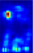
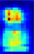
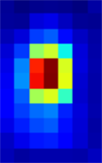
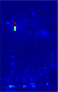
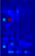
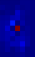
Figure 1: Visualization of classification scores for different methods. 1st: input image. 2nd-4th depict the classification score heatmaps of the FCOS baseline; 5th-7th depict the score heatmaps of our FCOS_PSS. The three maps correspond to FPN levels of P5, P6, and P7. Our FCOS_PSS trained with stop-gradient can significantly suppress duplicated predictions.

4.2.1 Effect of Stop Gradient

In this section, we analyze the effect of the asymmetric optimization scheme, i.e., stop the gradient relevant to the attached PSS head passing to the original FCOS network parameters. As depicted in Fig. LABEL:fig:model, we use the features of the regression branch to train the PSS head. The vanilla solution is not to have the stop-grad operation and update all the network parameters as usual.

Specifically, our ATSS_PSS  method without stop-gradient achieves 41.6% mAP (w/o NMS), which outperforms DeFCN by only 0.1 points and there is still a performance gap of 1.2 points compared to the ATSS  baseline (42.8%). By applying the stop-gradient operation, ATSS_PSS  achieves 42.6%, almost the same as the baseline’s 42.8% mAP. We make a similar observation for the FCOS_PSS  method and it is worth noting that the end-to-end prediction result (w/o NMS) with stop-gradient achieves 42.3%, which even improves the performance by 0.3% against the NMS-based FCOS baseline.

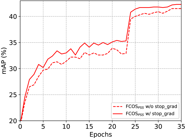
Figure 2: Comparison of mAP for our FCOS_PSS (top) and ATSS_PSS (bottom) models trained with and without stop-gradient w.r.t.  training epochs, showing that stop-gradient helps training a better model.

To further verify whether stop-gradient can better train our end-to-end detectors, we show the convergence curves of our FCOS_PSS and ATSS_PSS models trained with and without the stop-gradient operation on the COCO val. set. As shown in Fig. 2, we can observe that stop-gradient indeed help train a better model and is able to consistently improve the performance during the training process.

We present the visualization of the predicted classification scores from the FCOS baseline and our FCOS_PSS  methods in Fig. 1. The 2nd-4th depict the classification score heatmaps of the FCOS baseline and the 5th-7th depict the score heatmaps of our FCOS_PSS. The three score maps correspond to different FPN levels (P5, P6, P7). It is clear that compared with FCOS baseline, our FCOS_PSS trained with stop-gradient is capable of significantly suppressing duplicate predictions.

Model	Training Mode	mAP (w/o NMS)
ATSSPSS	end-to-end	42.6
ATSSPSS	two-step	42.3

Table 3: Comparison of detection accuracy of our ATSS_PSS model when trained end-to-end vs. with two-step training.

Model	Position	mAP (%)		mAR (%)
		end-to-end pred. (w/o NMS)	one-to-many pred. (w/ NMS)	end-to-end pred. (w/o NMS)	one-to-many pred. (w/ NMS)
FCOSPSS	PSS on regress. branch	42.3	42.2	61.6	59.6
	PSS on classif.  branch	41.5	42.2	60.9	59.4
ATSSPSS	PSS on regress.	42.6	42.3	62.1	59.7
	PSS on clssif.	41.8	42.3	61.4	60.0

Table 4: Comparison of detection accuracy for different methods by attaching the PSS head either to the classification branch or regression branch. As we can see that the PSS head attached to the regression branch works slightly better. Therefore, in all other experiments we have attached the PSS head to the regression branch.

4.2.2 Stop Gradient vs. Two-step Training

Stop-gradient allows the PSS module to be optimized asymmetrically compared to the rest of the network; and may benefit from the feature representation learning of the original FCOS/ATSS model. If we train in two steps, i.e., first train the FCOS/ATSS model to convergence, and then train the PSS module alone by freezing the FCOS/ATSS model, would this two-step strategy work well? As discussed in §3.5, this two-step optimization corresponds to optimization of sub-problems of (5) and (6) to convergence for only one alternation.

We train such a model by training a baseline model in step one for 36 epochs, and then train the PSS head in step two for another 12 epochs. As shown in Table 3, the two-step training of the ATSS_PSS model achieves 42.3% mAP (vs. 42.6% for end-to-end training).

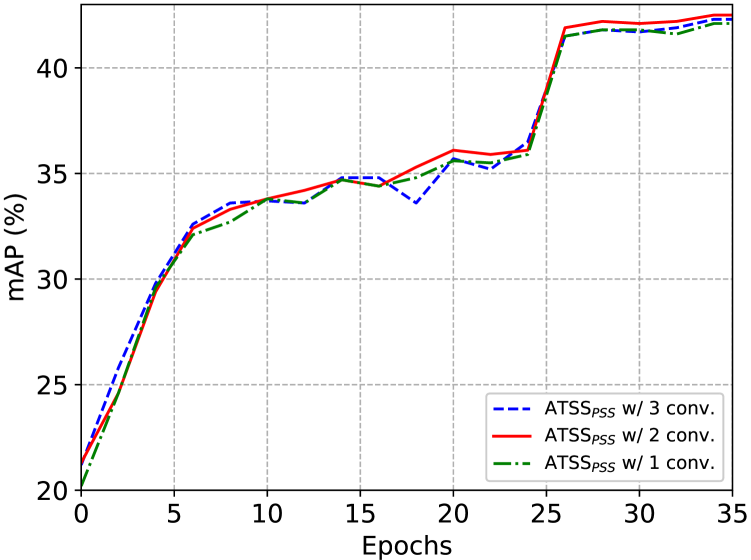
Figure 3: Comparison of mAP for our ATSS_PSS method trained with different conv. layers of the PSS head w.r.t. training epochs.

4.2.3 Attaching PSS to Regression vs.  Classification Branch

In this section, we analyze the effect of attaching the PSS head either to the classification branch or the regression branch. As shown in Table 4, compared with attaching to the regression branch, moving the PSS head to the classification branch results in performance degradation of end-to-end prediction, while the performance of one-to-many prediction remains unchanged. We thus conclude that it is more suitable to optimize the PSS head with features of the regression branch. Unless otherwise specified, we attach the PSS head to the regression branch in all other experiments. Recall that in the original FCOS, it was also observed that attaching the centre-ness head to regression works better than attaching to the classification branch.

4.2.4 How Many Conv. Layers for the PSS Head

Since we expect to learn a binary classifier for one-to-one prediction, the capacity of the head may play an important role. We use standard conv. layers to facilitate the learning of the binary mask. To verify how many conv. layers work well, we perform ablation study w.r.t.  the number of conv. layers based on FCOS_PSS and ATSS_PSS. As shown in Table 5, the PSS head with two conv. layers achieves satisfactory accuracy. It is interesting to see that increasing the PSS head to three conv. layers slightly deteriorates the detection performance, which may be due to overfitting. We plot the convergence curves in Fig. 3, showing that at the beginning, PSS with three layers obtains better mAP but later becomes slightly worse than that of two layers. Although carefully tuning the hyper-parameters may result in slightly different results, we may conclude here that two conv. layers for the PSS head already work well.

Model	$\#$ Conv. layers	mAP (%)		mAR (%)
		w/o NMS	w/ NMS	w/o NMS	w/ NMS
FCOSPSS	1	41.6	41.9	61.4	59.5
	2	42.3	42.2	61.6	59.6
	3	41.9	41.7	61.7	59.2
ATSSPSS	1	42.1	42.0	61.7	59.3
	2	42.6	42.3	62.1	59.7
	3	42.3	41.7	61.9	59.3

Table 5: The effect of the number of conv. layers for the PSS head. Each conv. layer has 256 channels with stride 1. All models are based on ResNet-50 with FPN; and the ‘3$\times$’ training schedule. In general, two conv. layers show satisfactory accuracy.

Model	Center-ness	mAP (%)
		end-to-end pred. (w/o NMS)	one-to-many pred. (w/ NMS)
FCOSPSS		41.7	41.4
	✓	42.3	42.2
ATSSPSS		42.1	41.7
	✓	42.6	42.3

Table 6: Comparison of detection accuracy for different models trained with and without the center-ness head respectively.

4.2.5 Effect of the Center-ness Branch

To evaluate the effect of the center-ness branch, we perform ablation study on our end-to-end detectors FCOS_PSS and ATSS_PSS trained with and without center-ness branch, respectively.

Compared with the positive samples far from the center of the instance, it make sense for the positive samples close to the center of the instance to have a larger loss weight. Therefore, although we remove the centerness branch, we still retain the centerness as the loss weight of GIoU loss during the training process. We report the results in Table 6. For FCOS_PSS, center-ness improves the mAP by 0.6 points. This is consistent with the observation for the FCOS baseline (see §3.1.3 of [25]).

For ATSS_PSS, center-ness can improve by 0.5 points. This is expected as a better positive example sampling strategy slightly diminishes the effectiveness the centerness.

Model	$\lambda_{1}$	mAP (%)
		end-to-end pred. (w/o NMS)	one-to-many pred. (w/ NMS)
FCOSPSS	0.5	41.7	41.9
	1.0	42.3	42.2
	2.0	41.7	41.5

Table 7: Comparison of detection accuracy by varying the loss weight of the PSS term as in Equ. (1) on the COCO val.  set.

4.2.6 Loss Weight of PSS Loss ${\cal L}_{pss}$

In this section, we analyze the sensitivity of the loss weight $\lambda_{1}$ of the PSS loss ${\cal L}_{pss}$ in Equ. (1). Specifically, we evaluate our FCOS_PSS method with different values for $\lambda_{1}\in\{0.5,1.0,2.0\}$ and report the results in Table 7. It appears that $\lambda_{1}=1$ already works well.

Method	$\alpha$	mAP (%)	mAR (%)
Add	0.2	41.6	61.3
	0.4	41.7	61.4
	0.6	41.7	60.9
	0.8	41.3	60.6
Mul.	0.2	41.6	60.4
	0.4	41.8	61.1
	0.6	41.8	61.0
	0.8	42.3	61.6

Table 8: Comparison of different matching score functions of our FCOS_PSS model on the COCO val. set.

4.2.7 Matching Score Function

To explore the best formulation of matching score functions of our FCOS_PSS model, we borrow the ‘Add’ function form of [26] and replace the matching score function in Equ. (3) by $(1-\alpha)\cdot\hat{P}_{i}(c_{j})+\alpha\cdot{\rm IoU}(\hat{b}_{i},b_{j})$. As shown in Table 8, compared with ‘Add’, the ‘Mul.’ function works slightly better, achieving the best detection performance of 42.3% mAP with $\alpha=0.8$. Therefore, we use ‘Mul.’ function with $\alpha=0.8$ in all other experiments.

4.2.8 Effect of the Ranking Loss

To demonstrate the effectiveness of the ranking loss, we performs experiments on our FCOS_PSS and ATSS_PSS detectors trained with and without ranking loss respectively. The results are reported in Table 9, without introducing much training complexity, the ranking loss can further improves the final detection performance by 0.2$\scriptstyle\sim$0.3 points in mAP.

Model	Ranking loss	mAP (%)
FCOSPSS		42.0
	✓	42.3
ATSSPSS		42.4
	✓	42.6

Table 9: Comparison of mAP for our FCOS_PSS and ATSS_PSS models trained with and without the ranking loss, indicating that our ranking loss can further improve the detection performance.

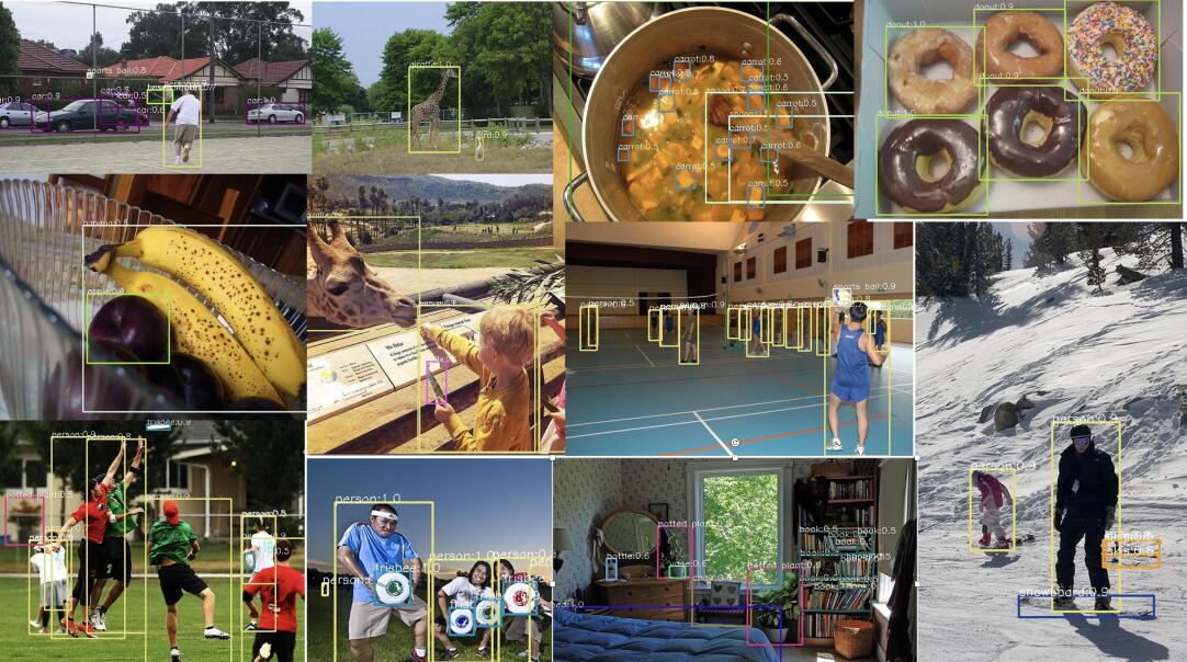
Figure 4: Visalization of some detection results from the COCO dataset. Results are obtained using the ATSS_PSS with the R2N-101-DCN backbone model, achieving 48.5% mAP on the COCO val. set.

4.3 Comparison with State-of-the-art

We compare FCOS_PSS/ATSS_PSS with other state-of-the-art object detectors on the COCO benchmark. For these experiments, we make use of multi-scale training. In particular, during training, the shorter side of the input image is sampled from $[480,800]$ with a step of 32 pixels.

From Table 1, we make the following conclusions.

• Compared to the standard baseline FCOS, the proposed FCOS_PSS even achieves slightly detection accuracy, with negligible computation overhead.

  The detection mAP difference between the baseline ATSS and the proposed ATSS_PSS is less than 0.2 points.

• Our methods outperform the recent end-to-end NMS-free detector DeFCN.

• Our methods show improved performance with backbones of large capacity. In particular, we have trained models of ResNeXt-32$\times$4d-101 with deformable convolutions, and Res2Net-101 with deformable convolutions. Our models achieve 47.5% and 48.5% mAP respectively, which are among the state-of-the-art.

We show some qualitative results in Fig. 4.

Model	Sched.	Box mAP (%)	Mask mAP (%)
CondInst [23]	1$\times$	38.9	34.1
CondInst [23]	3$\times$	42.1	37.0
CondInstPSS (Ours)	1$\times$	39.4	34.4
CondInstPSS (Ours)	3$\times$	42.4	36.8

Table 10: Comparison of mAP for the CondInst baseline and our CondInst_PSS models on the COCO val.  set. The backbone is R50.

4.4 PSS for Instance Segmentation

Instance segmentation is a fundamental yet challenging task in computer vision and has received much attention in the community [7, 23]. In this section we demonstrate that our PSS head can benefit the NMS-based Instance segmentation methods. Recently, CondInst [23] eliminates ROI operations by employing dynamic instance-aware networks, which achieves improved instance segmentation performance. However, CondInst still needs box-based NMS to achieve accurate and fast performance during inference. Similar to FCOS_PSS, we only introduce our PSS head to the original CondInst network, denoted as CondInst_PSS. We carry out experiments on the COCO dataset and report the results in Table 10. The results indicate that by eliminating heuristic NMS, we can simplify the instance segmentation method while still achieving competitive performance.

5 Conclusion

In this work, we have proposed a very simple modification to the original FCOS detector (and its improved version of ATSS) for eliminating the heuristic NMS post-processing. We achieve that by attaching a compact positive sample selector head to the bounding box regression branch of the FCOS network, which consists of only two conv. layers. Thus, once trained, the new detector can be deployed easily without any heuristic processing involved. The proposed detector is made simpler and end-to-end trainable. We also show that the same idea can be applied to instance segmentation for removing NMS. We expect to see that the proposed design in this work may benefit many other instance-level recognition tasks beyond bounding-box object detection.

References

- [1] Nicolas Carion, Francisco Massa, Gabriel Synnaeve, Nicolas Usunier, Alexander Kirillov, and Sergey Zagoruyko. End-to-end object detection with transformers. In Proc. Eur. Conf. Comp. Vis., 2020.
- [2] Hao Chen, Kunyang Sun, Zhi Tian, Chunhua Shen, Yongming Huang, and Youliang Yan. Blendmask: Top-down meets bottom-up for instance segmentation. In Proc. IEEE Conf. Comp. Vis. Patt. Recogn., pages 8573–8581, 2020.
- [3] Kai Chen, Jiaqi Wang, Jiangmiao Pang, Yuhang Cao, Yu Xiong, Xiaoxiao Li, Shuyang Sun, Wansen Feng, Ziwei Liu, Jiarui Xu, Zheng Zhang, Dazhi Cheng, Chenchen Zhu, Tianheng Cheng, Qijie Zhao, Buyu Li, Xin Lu, Rui Zhu, Yue Wu, Jifeng Dai, Jingdong Wang, Jianping Shi, Wanli Ouyang, Chen Change Loy, and Dahua Lin. MMDetection: Open mmlab detection toolbox and benchmark. arXiv: Comp. Res. Repository, 2019.
- [4] Xinlei Chen and Kaiming He. Exploring simple siamese representation learning. arXiv: Comp. Res. Repository, 2020.
- [5] Shang-Hua Gao, Ming-Ming Cheng, Kai Zhao, Xin-Yu Zhang, Ming-Hsuan Yang, and Philip Torr. Res2Net: A new multi-scale backbone architecture. IEEE Trans. Pattern Anal. Mach. Intell., 43(2):652–662, 2021.
- [6] Dongyan Guo, Jun Wang, Ying Cui, Zhenhua Wang, and Shengyong Chen. SiamCAR: Siamese fully convolutional classification and regression for visual tracking. In Proc. IEEE Conf. Comp. Vis. Patt. Recogn., 2020.
- [7] Kaiming He, Georgia Gkioxari, Piotr Dollár, and Ross Girshick. Mask R-CNN. In Proc. IEEE Int. Conf. Comp. Vis., pages 2961–2969, 2017.
- [8] Kaiming He, Xiangyu Zhang, Shaoqing Ren, and Jian Sun. Deep residual learning for image recognition. In Proc. IEEE Conf. Comp. Vis. Patt. Recogn., pages 770–778, 2016.
- [9] Kang Kim and Hee Seok Lee. Probabilistic anchor assignment with iou prediction for object detection. In Proc. Eur. Conf. Comp. Vis., 2020.
- [10] Tao Kong, Fuchun Sun, Huaping Liu, Yuning Jiang, Lei Li, and Jianbo Shi. FoveaBox: Beyond anchor-based object detector. IEEE Trans. Image Process., pages 7389–7398, 2020.
- [11] Xiang Li, Wenhai Wang, Lijun Wu, Shuo Chen, Xiaolin Hu, Jun Li, Jinhui Tang, and Jian Yang. Generalized focal loss: Learning qualified and distributed bounding boxes for dense object detection. In Proc. Advances in Neural Inf. Process. Syst., 2020.
- [12] Tsung-Yi Lin, Piotr Dollár, Ross Girshick, Kaiming He, Bharath Hariharan, and Serge Belongie. Feature pyramid networks for object detection. In Proc. IEEE Conf. Comp. Vis. Patt. Recogn., pages 2117–2125, 2017.
- [13] Tsung-Yi Lin, Priya Goyal, Ross B. Girshick, Kaiming He, and Piotr Dollár. Focal loss for dense object detection. In Proc. IEEE Int. Conf. Comp. Vis., 2017.
- [14] Tsung-Yi Lin, Michael Maire, Serge Belongie, James Hays, Pietro Perona, Deva Ramanan, Piotr Dollár, and Lawrence Zitnick. Microsoft COCO: Common objects in context. In Proc. Eur. Conf. Comp. Vis., pages 740–755, 2014.
- [15] Wei Liu, Dragomir Anguelov, Dumitru Erhan, Christian Szegedy, Scott Reed, Cheng-Yang Fu, and Alexander C. Berg. SSD: Single shot multibox detector. In Proc. Eur. Conf. Comp. Vis., 2016.
- [16] Yuliang Liu, Hao Chen, Chunhua Shen, Tong He, Lianwen Jin, and Liangwei Wang. ABCNet: Real-time scene text spotting with adaptive Bezier-curve network. In Proc. IEEE Conf. Comp. Vis. Patt. Recogn., 2020.
- [17] Han Qiu, Yuchen Ma, Zeming Li, Songtao Liu, and Jian Sun. Borderdet: Border feature for dense object detection. In Proc. Eur. Conf. Comp. Vis., pages 549–564, 2020.
- [18] Joseph Redmon, Santosh Divvala, Ross Girshick, and Ali Farhadi. You only look once: Unified, real-time object detection. In Proc. IEEE Conf. Comp. Vis. Patt. Recogn., 2016.
- [19] Shaoqing Ren, Kaiming He, Ross B. Girshick, and Jian Sun. Faster R-CNN: Towards real-time object detection with region proposal networks. In Proc. Advances in Neural Inf. Process. Syst., 2015.
- [20] Russell Stewart, Mykhaylo Andriluka, and Andrew Y. Ng. End-to-end people detection in crowded scenes. In Proc. IEEE Conf. Comp. Vis. Patt. Recogn., 2016.
- [21] Peize Sun, Yi Jiang, Enze Xie, Zehuan Yuan, Changhu Wang, and Ping Luo. OneNet: Towards end-to-end one-stage object detection. arXiv: Comp. Res. Repository, 2020.
- [22] Zhi Tian, Hao Chen, and Chunhua Shen. DirectPose: Direct end-to-end multi-person pose estimation. arXiv: Comp. Res. Repository, 2019.
- [23] Zhi Tian, Chunhua Shen, and Hao Chen. Conditional convolutions for instance segmentation. In Proc. Eur. Conf. Comp. Vis., 2020.
- [24] Zhi Tian, Chunhua Shen, Hao Chen, and Tong He. FCOS: Fully convolutional one-stage object detection. In Proc. IEEE Int. Conf. Comp. Vis., 2019.
- [25] Zhi Tian, Chunhua Shen, Hao Chen, and Tong He. Fcos: A simple and strong anchor-free object detector. IEEE Trans. Pattern Anal. Mach. Intell., 2021.
- [26] Jianfeng Wang, Lin Song, Zeming Li, Hongbin Sun, Jian Sun, and Nanning Zheng. End-to-end object detection with fully convolutional network. arXiv: Comp. Res. Repository, 2020.
- [27] Xinlong Wang, Tao Kong, Chunhua Shen, Yuning Jiang, and Lei Li. SOLO: Segmenting objects by locations. In Proc. Eur. Conf. Comp. Vis., 2020.
- [28] Xinlong Wang, Rufeng Zhang, Tao Kong, Lei Li, and Chunhua Shen. SOLOv2: Dynamic and fast instance segmentation. In Proc. Advances in Neural Inf. Process. Syst., 2020.
- [29] Enze Xie, Peize Sun, Xiaoge Song, Wenhai Wang, Xuebo Liu, Ding Liang, Chunhua Shen, and Ping Luo. PolarMask: Single shot instance segmentation with polar representation. In Proc. IEEE Conf. Comp. Vis. Patt. Recogn., 2020.
- [30] Saining Xie, Ross B. Girshick, Piotr Dollár, Zhuowen Tu, and Kaiming He. Aggregated residual transformations for deep neural networks. In Proc. IEEE Conf. Comp. Vis. Patt. Recogn., 2017.
- [31] Rufeng Zhang, Zhi Tian, Chunhua Shen, Mingyu You, and Youliang Yan. Mask encoding for single shot instance segmentation. In Proc. IEEE Conf. Comp. Vis. Patt. Recogn., 2020.
- [32] Shifeng Zhang, Cheng Chi, Yongqiang Yao, Zhen Lei, and Stan Z. Li. Bridging the gap between anchor-based and anchor-free detection via adaptive training sample selection. In Proc. IEEE Conf. Comp. Vis. Patt. Recogn., pages 9759–9768, 2020.
- [33] Xizhou Zhu, Han Hu, Stephen Lin, and Jifeng Dai. Deformable convnets v2: More deformable, better results. In Proc. IEEE Conf. Comp. Vis. Patt. Recogn., pages 9308–9316, 2019.
- [34] Xizhou Zhu, Weijie Su, Lewei Lu, Bin Li, Xiaogang Wang, and Jifeng Dai. Deformable DETR: Deformable transformers for end-to-end object detection. In Proc. Int. Conf. Learn. Representations, 2020.