Wave Dark Matter

Abstract

We review the physics and phenomenology of wave dark matter: a bosonic dark matter candidate lighter than about $30$ eV. Such particles have a de Broglie wavelength exceeding the average inter-particle separation in a galaxy like the Milky Way, thus well described as a set of classical waves. We outline the particle physics motivations for them, including the QCD axion as well as ultra-light axion-like-particles such as fuzzy dark matter. The wave nature of the dark matter implies a rich phenomenology:

• Wave interference gives rise to order unity density fluctuations on
  de Broglie scale in halos. One manifestation is vortices where the
  density vanishes and around which the velocity circulates. There is
  one vortex ring per de Broglie volume on average.

• For sufficiently low masses, soliton condensation occurs at centers
  of halos. The soliton oscillates and random walks, another
  manifestation of wave interference. The halo and subhalo
  abundance is expected to be suppressed at small masses, but the
  precise prediction from numerical wave simulations remains to be
  determined.

• For ultra-light $\sim 10^{-22}$ eV dark matter, the wave interference
  substructures can be probed by tidal streams/gravitational
  lensing. The signal can be distinguished from that due to subhalos
  by the dependence on stream orbital radius/image separation.

• Axion detection experiments are sensitive to interference
  substructures for wave dark matter that is moderately light. The
  stochastic nature of the waves affects the interpretation of
  experimental constraints and motivates the measurement of
  correlation functions.

Current constraints and open questions, covering detection experiments and cosmological/galactic/black-hole observations, are discussed.

1 INTRODUCTION

The astronomical evidence for the existence of dark matter, accumulated over decades, is rich and compelling (e.g., Zwicky, 1933, Smith, 1936, Rubin & Ford, 1970, Freeman, 1970, Ostriker & Peebles, 1973, Hoekstra et al., 2004, Clowe et al., 2006, Bennett et al., 2013, Aghanim et al., 2020). Yet, the identity and basic properties of dark matter remain shrouded in mystery. An example is the constituent’s mass: proposals range from ultra-light $\sim 10^{-22}$ eV (Hu, Barkana & Gruzinov, 2000) to astronomical $\sim 10{\,\rm M_{\odot}}$ (Bird et al., 2016, Garcia-Bellido & Ruiz Morales, 2017, Sasaki et al., 2018, Jedamzik, 2020). In this vast spectrum, there is nonetheless a useful demarcation point. Dynamical measurements tell us the dark matter mass density in the solar neighborhood is about $0.4{\,\rm GeV\,cm^{-3}}$. From this, one can deduce the average inter-particle separation, given a dark matter particle mass. We can compare it against the de Broglie wavelength of the particle:

$$\lambda_{\rm dB}\equiv{2\pi\over{mv}}=0.48{\,\rm kpc}\left({10^{-22}{\,\rm eV}\over m}\right)\left({250{\,\rm km/s}\over v}\right)=1.49{\,\rm km}\left({10^{-6}{\,\rm eV}\over m}\right)\left({250{\,\rm km/s}\over v}\right)\,,$$ (1)

where $v$ is the velocity dispersion of the galactic halo, and $m$ is the dark matter particle mass, for which two representative values are chosen for illustration. It can be shown that the de Broglie wavelength exceeds the inter-particle separation if $m\,\lower 3.22916pt\hbox{$\sim$}\hbox to0.0pt{\hss\raise 1.1625pt\hbox{$<$}}\,30$ eV. In other words, in a Milky-Way-like environment, the average number of particles in a de Broglie volume $\lambda_{\rm dB}^{3}$ is:

$$N_{\rm dB}\sim\left({34{\,\rm eV}\over m}\right)^{4}\left({250{\,\rm km/s}\over v}\right)^{3}\,.$$ (2)

For $m\ll 30$ eV, the occupancy $N_{\rm dB}$ is so large that the set of particles is best described by classical waves, much as in electromagnetism, a state with a large number of photons is well described by the classical electric and magnetic fields. The associated wave phenomena is the subject of this review. We emphasize classical, for large occupancy implies negligible quantum fluctuations. The question of how the classical description relates to the underlying quantum one is a fascinating subject. We unfortunately do not have the space to explore it here (see Sikivie & Yang, 2009, Guth et al., 2015, Dvali & Zell, 2018, Lentz et al., 2020, Allali & Hertzberg, 2020).

Such a light dark matter particle is necessarily bosonic, for the Pauli exclusion principle precludes multiple occupancies for fermions—this is the essence of the bound by Tremaine & Gunn (1979). For concreteness, we focus on a spin zero (scalar) particle, although much of the wave phenomenology applies to higher spin cases as well (Graham et al., 2016b, Kolb & Long, 2020, Aoki & Mukohyama, 2016). There is a long history of investigations of dark matter as a scalar field (e.g., Baldeschi et al., 1983, Turner, 1983, Press et al., 1990, Sin, 1994, Peebles, 2000, Goodman, 2000, Lesgourgues et al., 2002, Amendola & Barbieri, 2006, Chavanis, 2011, Suarez & Matos, 2011, Rindler-Daller & Shapiro, 2012, Berezhiani & Khoury, 2015a, Fan, 2016, Alexander & Cormack, 2017). Perhaps the most well motivated example is the Quantum Chromodynamics (QCD) axion (Peccei & Quinn, 1977, Kim, 1979, Weinberg, 1978, Wilczek, 1978, Shifman et al., 1980, Zhitnitsky, 1980, Dine et al., 1981, Preskill et al., 1983, Abbott & Sikivie, 1983, Dine & Fischler, 1983). Its possible mass spans a large range—experimental detection has focused on masses around $10^{-6}$ eV, with newer experiments reaching down to much lower values. For recent reviews, see Graham et al. (2015), Marsh (2016), Sikivie (2020). String theory also predicts a large number of axion-like-particles (ALP), one or some of which could be dark matter (Svrcek & Witten, 2006, Arvanitaki et al., 2010, Halverson et al., 2017, Bachlechner et al., 2019). At the extreme end of the spectrum is the possibility of an ALP with mass around $10^{-22}-10^{-20}$ eV, with a relic abundance that naturally matches the observed dark matter density (see Section 3). More generally, ultra-light dark matter in this mass range is often referred to as fuzzy dark matter (FDM). It was proposed by Hu, Barkana & Gruzinov (2000) to address small scale structure issues thought to be associated with conventional cold dark mater (CDM) (Spergel & Steinhardt, 2000). This is a large subject we will not discuss in depth, though it will be touched upon in Section 5. It remains unclear whether the small scale structure issues point to novelty in the dark matter sector, or can be resolved by baryonic physics, once the complexities of galaxy formation are properly understood (for a recent review, see Weinberg et al., 2015).

In this article, we take a broad perspective on wave dark matter ($m\,\lower 3.22916pt\hbox{$\sim$}\hbox to0.0pt{\hss\raise 1.1625pt\hbox{$<$}}\,30$ eV), and discuss novel features that distinguish it from particle dark matter ($m\,\lower 3.22916pt\hbox{$\sim$}\hbox to0.0pt{\hss\raise 1.1625pt\hbox{$>$}}\,30$ eV). The underlying wave dynamics is the same whether the dark matter is ultra-light like fuzzy dark matter, or merely light like the QCD axion. The length scale of the wave phenomena (i.e. the de Broglie wavelength) depends of course on the mass. For the higher masses, the length scales are small, which can be probed by laboratory detection experiments. (The higher masses can have astrophysical consequences too, despite the short de Broglie wavelength, for instance around black holes or in solitons, as we will see.) For the ultra-light end of the spectrum, fuzzy dark matter ($m\sim 10^{-22}-10^{-20}$ eV), the length scales are long and there can be striking astrophysical signatures, which we will highlight. A mass $m\,<\,10^{-22}$ eV is possible, but only if the particle constitutes a small fraction of dark matter, for the simple reason that an excessively large $\lambda_{\rm dB}$ precludes the existence of dark matter dominated dwarf galaxies (Hu et al., 2000). When the mass approaches the size of the Hubble constant today $m\sim 10^{-33}$ eV, the scalar field is so slowly rolling that it is essentially a form of dark energy (Hlozek et al., 2015). (The distinction between a slowly rolling scalar field as dark energy, and oscillating scalar field as dark matter, is discussed in Section 3.)

An outline of the article is as follows. Particle physics motivations for considering wave dark matter are discussed in Section 3. The bulk of this review is devoted to elucidating the dynamics and phenomenology of wave dark matter, in Section 4. The observational/experimental implications and constraints are summarized in Section 5. We conclude in Section 6 with a discussion of open questions and directions for further research. This article is intended to be pedagogical: we emphasize results that can be understood in an intuitive way, while providing ample references. We devote more space to elucidating the physics than to summarizing the current constraints, which evolve, sometimes rapidly.

[t]

2 Terminology

We use the term axion to loosely refer to both the QCD axion, and an axion-like-particle (Section 3). The term fuzzy dark matter (FDM) is reserved for the ultra-light part of the mass spectrum $m\sim 10^{-22}-10^{-20}$ eV. Wave dark matter is the more general term, $m\,\lower 3.22916pt\hbox{$\sim$}\hbox to0.0pt{\hss\raise 1.1625pt\hbox{$<$}}\,30$ eV, for which dark matter exhibits wave phenomena. Wave dark matter, such as the axion, is in fact one form of cold dark matter (CDM), assuming it is not produced by thermal freeze-out (see Section 3). We use the term particle dark matter for cases where $m\,\lower 3.22916pt\hbox{$\sim$}\hbox to0.0pt{\hss\raise 1.1625pt\hbox{$>$}}\,30{\,\rm eV}$, the primary example of which is Weakly Interacting Massive Particle (WIMP). We sometimes refer to it as conventional CDM.

3 Particle physics motivations

In this section, we describe the axion—the QCD axion or an axion-like-particle—as a concrete example of wave dark matter: (1) how it is motivated by high energy physics considerations independent of the dark matter problem; (2) how a relic abundance that matches the observed dark matter density can be naturally obtained; (3) how it is weakly interacting and cold. Readers not interested in the details can skip to Section 4 without loss of continuity.

We are interested in a scalar field $\phi$ that has a small mass $m$. A natural starting point is a massless Goldstone boson, associated with the spontaneous breaking of some symmetry. Non-perturbative quantum effects can generate a small mass—hence, a pseudo Goldstone boson—or more generally a potential $V(\phi)$, giving a Lagrangian density of the form:

$${\cal L}=-{1\over 2}\partial_{\mu}\phi\,\partial^{\mu}\phi-V(\phi)\,.$$ (3)

A concrete realization is the axion, which is a real angular field, in the sense that $\phi$ and $\phi+2\pi f$ are identified i.e. $\phi/f$ is effectively an angle. The periodicity scale $f$, an energy scale, is often referred to as the axion decay constant.

The classic example is the QCD axion, a particle that couples to the gluon field strength and derives its mass from the presence of this coupling (and confinement). It was introduced to address the strong CP (charge-conjugation parity) problem: that a certain parameter in the standard model, the angle $\theta_{\rm QCD}$, is constrained to be less than $10^{-9}$ from experimental bounds on the neutron electric dipole moment. It has certain generic couplings to the standard model, allowing the possibility of experimental detection (see below). More general examples—namely, axion-like-particles which have similar couplings to the standard model but do not contribute to the resolution of the strong CP problem—arise naturally in string theory as the Kaluza-Klein zero modes of higher form fields when the extra dimensions are compactified (Green et al., 1988, Svrcek & Witten, 2006, Arvanitaki et al., 2010, Dine, 2016, Halverson et al., 2017, Bachlechner et al., 2019).

Peccei-Quinn U(1)the symmetry associated with shifting $\phi$ by a constant. Its spontaneous breaking is what makes the axion $\phi$ possible. Its small explicit breaking by non-perturbative effects gives $\phi$ a potential.

For illustration, consider a potential $V(\phi)$ of the following form:

$$V(\phi)=\Lambda^{4}(1-{\,\rm cos\,}[\phi/f])\,.$$ (4)

(The QCD axion potential does not have this precise form, but shares similar qualitative features.) The cosine is consistent with the idea of $\phi/f$ being an angle. The additive constant is not important for our considerations, and is chosen merely to make $V$ vanish at the minimum $\phi=0$. The mass of $\phi$ can be read off from expanding the cosine around $\phi=0$: $m=\Lambda^{2}/f$. Typically, $f$ is some high energy scale up to Planck scale, while $\Lambda$ is exponentially suppressed compared to that (see footnote 5), giving a small $m$. For instance, $f\sim 10^{17}$ GeV and $\Lambda\sim 100$ eV gives $m\sim 10^{-22}$ eV. The QCD axion potential does not have the exact form above (for a recent computation, see Grilli di Cortona et al., 2016), but $m\sim\Lambda^{2}/f$ remains true with $\Lambda$ being the QCD scale $\sim 100$ MeV. For instance, $f\sim 10^{13}$ GeV gives $m\sim 10^{-6}$ eV for the QCD axion.

What determines the contribution of $\phi$ to the energy content of the universe today? Here we outline the misalignment mechanism (reviewed in Kolb & Turner, 1990). Consider the equation of motion for a homogeneous $\phi$ (following from Equation 3) in an expanding background):

$$\ddot{\phi}+3H\dot{\phi}+\partial_{\phi}V=0\,,$$ (5)

where $H$ is the Hubble expansion rate. In the early universe, when $H$ is large, Hubble friction is sufficient to keep $\phi$ slowly rolling i.e. balancing the last two terms on the left. Thus $V(\phi)$ plays the role of dark energy. The value of $\phi$ is essentially stuck at its primordial value—we assume $\phi_{\rm primordial}/f$, the so called misalignment angle, is order unity. The expansion rate drops as time goes on, until $H$ reaches $\sim m$. After that $\phi$ rolls towards the minimum of the potential and commences oscillations around it. The expansion of the universe takes energy out of such oscillations, diminishing the oscillation amplitude. Subsequently, $\phi$ oscillates close to zero, implying it is a good approximation to treat the potential as:

$$V(\phi)\sim{1\over 2}m^{2}\phi^{2}\,.$$ (6)

The energy density contained in the $\phi$ oscillations is

$$\rho={1\over 2}\dot{\phi}{}^{2}+{1\over 2}m^{2}\phi^{2}\,.$$ (7)

It follows from Equation 5 that $\rho$ redshifts like $a^{-3}$ where $a$ is the scale factor. The $\phi$ oscillations, which can be interpreted as a set of particles, therefore have the redshifting behavior of (non-relativistic) matter, making this a suitable dark matter candidate. Following this cosmological history, it can be shown that the relic density today is (e.g., Arvanitaki et al., 2010, Marsh, 2016, Hui et al., 2017):

$$\Omega_{\rm axion}\sim 0.1\left({f\over 10^{17}{\,\rm GeV}}\right)^{2}\left({m\over 10^{-22}{\,\rm eV}}\right)^{1/2}\,$$ (8)

where $\Omega_{\rm axion}$ is the axion density today as a fraction of the critical density. It is worth emphasizing the relic density is more sensitive to the choice of $f$ than to $m$. The value of $10^{17}$ GeV, close to but below the Planck scale, is motivated by string theory constructions (Svrcek & Witten, 2006). But a slightly different $f$ would have to be paired with a quite different $m$, if one were to insist on matching the observed dark matter abundance. Nonetheless, this relic abundance computation motivates the consideration of light, even ultra-light, axions.

The reasoning above essentially follows the classic computation of the QCD axion relic density (Preskill et al., 1983, Abbott & Sikivie, 1983, Dine & Fischler, 1983)—the difference is that while $V(\phi)$ is constant here, it is temperature dependent for the QCD axion. Besides the misalignment mechanism, it is also possible axions arise from the decay of topological defects, if the Peccei-Quinn U(1) symmetry is broken after inflation (for recent lattice computations, see Gorghetto et al., 2020, Buschmann et al., 2020).

Aside from having the requisite relic abundance, a good dark matter candidate should be cold and weakly interacting. The coldness is implicit in the misalignment mechanism: the axion starts off as a homogeneous scalar field in the early universe, with the homogeneity guaranteed for instance by inflation. (There are inevitable small fluctuations as well, which is discussed in Section 5.) The weakly interacting nature is implied by the large axion decay constant $f$. Possible interactions include:

$${\cal L}^{\rm self}_{\rm int.}\sim{m^{2}\over f^{2}}\phi^{4}\quad,\quad{\cal L}^{\rm\gamma}_{\rm int.}\sim{\phi\over f}F^{\mu\nu}\tilde{F}_{\mu\nu}\quad,\quad{\cal L}^{\rm\Psi}_{\rm int.}\sim{\partial_{\mu}\phi\over f}\bar{\Psi}\gamma^{\mu}\gamma_{5}\Psi\,.$$ (9)

The first interaction, a self-interaction of $\phi$, follows from expanding out the potential $V(\phi)$ to quartic order; it is an attractive interaction for the axion. The second interaction is with the photon, $F$ and $\tilde{F}$ being the photon field strength and its dual (there is an analogous interaction with gluon field strength and its dual for the QCD axion). The third interaction is with a fermion $\Psi$, which could represent quarks or leptons. The last two interactions are both symmetric under a shift of $\phi$ by a constant, as befitting a (pseudo) Goldstone boson. The generic expectation is that all three coupling strengths are of the order shown, but models can be constructed that deviate from it (Kim & Marsh, 2016, Kaplan & Rattazzi, 2016, Choi & Im, 2016). The important point is that $f$ is expected to be large, keeping these interactions weak, for both the QCD axion and axion-like-particles. For structure formation purpose, these interactions can be largely ignored, though their presence is important for direct detection and in certain extreme astrophysical environments, as we will discuss below.

4 Wave dynamics and phenomenology

The discussion above motivates us to consider a scalar field $\phi$ satisfying the Klein Gordon equation:

$$-\Box\phi+m^{2}\phi=0\,,$$ (10)

which follows from Equation 3 with the potential approximated by Equation 6. Much of the following discussion is not specific to axions—it applies to any scalar (or pseudo-scalar) particle whose dominant interaction is gravitational. Occasionally, we will comment on features that are specific to axions, for instance in cases where their self-interaction is important.

Unlike in Equation 5, here we are interested in the possibility of $\phi$ having spatial fluctuations. In the non-relativistic regime relevant for structure formation, it is useful to introduce a complex scalar $\psi$ ($\phi$ is a real scalar):

$$\phi={1\over\sqrt{2m}}\left(\psi e^{-imt}+\psi^{*}e^{imt}\right)\,.$$ (11)

The idea is to factor out the fast time dependence of $\phi$—oscillation with frequency $m$—and assume $\psi$ is slowly varying i.e. $|\ddot{\psi}|\ll m|\dot{\psi}|$. The Klein-Gordon equation reduces to the Schrödinger equation:

$$i\,\partial_{t}\psi=-{\nabla^{2}\over 2m}\psi+m\Phi\psi\,.$$ (12)

Several comments are in order. (1) In what sense is the assumption of $\partial_{t}\ll m$ non-relativistic? From the Schrödinger equation, we see $\partial_{t}\sim\nabla^{2}/m\sim k^{2}/m$. Thus $\partial_{t}\ll m$ is equivalent to $k^{2}/m\ll m$ i.e. momentum is small compared to rest mass. (2) We introduce the gravitational potential $\Phi$. Recall that $\Box=g^{\mu\nu}\nabla_{\mu}\nabla_{\nu}$ contains the metric $g^{\mu\nu}$, thus gravitational interaction of $\phi$ is implicit. For many applications, this is the only interaction we need to include. In principle, the metric should account for the cosmic expansion, which we have ignored to simplify the discussion. Cosmic counterparts of the equations presented here can be found in (e.g., Hu et al., 2000, Hui et al., 2017). (3) Despite the appearance of the Schrödinger equation, $\psi$ should be thought of as a (complex) classical field. The situation is analogous to the case of electromagnetism: a state with high occupancy is adequately described by the classical electric and magnetic fields. We will on occasion refer to $\psi$ as the wavefunction, purely out of habit.

The non-relativistic dynamics of wave dark matter is completely described by Equation 12, supplemented by the Poisson equation:

$$\nabla^{2}\Phi=4\pi G\rho\quad,\quad\rho=m|\psi|^{2}\,.$$ (13)

The expression for mass density $\rho$ can be justified by plugging Equation 11 into Equation 7, taking the non-relativistic limit and averaging over oscillations i.e. $|\psi|^{2}$ has the meaning of particle number density. Strictly speaking, the energy density should include gradient energy which is not contained in Equation 7. The gradient energy contribution to $\rho$ is of order $|\nabla\psi|^{2}/m$ which is negligible compared to the rest mass contribution $m|\psi|^{2}$ in the non-relativistic regime.

An alternative, fluid description of this wave system is instructive. This is called the Madelung (1927) formulation (see also Feynman et al., 1963). The mass density of the fluid is $\rho=m|\psi|^{2}$ as discussed. The complex $\psi$ can be written as $\psi=\sqrt{\rho/m}\,e^{i\theta}$. The fluid velocity $\vec{v}$ is related to the phase $\theta$ by:

$$\vec{v}={1\over m}\vec{\nabla}\theta={i\over 2m|\psi|^{2}}(\psi\vec{\nabla}\psi^{*}-\psi^{*}\vec{\nabla}\psi)\,.$$ (14)

Notice the fluid velocity is a gradient flow, resembling that of a superfluid. (A superfluid can have vortices as topological defects, see Section 4.4.) With this identification of the fluid velocity, what is normally understood as probability conservation in quantum mechanics is now recast as mass conservation:

$$\partial_{t}\rho+\vec{\nabla}\cdot(\rho\vec{v})=0\,.$$ (15)

The Schrödinger equation possesses a U(1) symmetry, the rotation of $\psi$ by a phase. In our context, conservation of the associated Noether current expresses particle number conservation, or mass conservation, as appropriate for the $\phi$ particles in the non-relativistic regime.

The Schrödinger equation is complex. Thus, besides mass conservation, it implies an additional real equation, the Euler equation:

$$\partial_{t}\vec{v}+(\vec{v}\cdot\vec{\nabla})\,\vec{v}=-\vec{\nabla}\Phi+\frac{1}{2m^{2}}\vec{\nabla}\left(\frac{\nabla^{2}\sqrt{\rho}}{\sqrt{\rho}}\right).$$ (16)

Equations 15 and 16 serve as an alternative, fluid description to the Schrodinger or wave formulation. The last term in Equation 16 is often referred to as the quantum pressure term. It is a bit of a misnomer (which we will perpetuate!), for what we have is a classical system. Also, the term arises from a stress tensor rather than mere pressure:

$$\Sigma_{ij}={1\over 4m^{2}}(\rho^{-1}\partial_{i}\rho\partial_{j}\rho-\partial_{i}\partial_{j}\rho)=-{\rho\over 4m^{2}}\partial_{i}\partial_{j}{\,\rm ln\,}\rho\,,$$ (17)

i.e. $\partial_{i}(\nabla^{2}\sqrt{\rho}/\sqrt{\rho})/(2m^{2})=-\rho^{-1}\partial_{j}\Sigma_{ij}$. The stress tensor represents how the fluid description accounts for the underlying wave dynamics. It shows in a clear way how the particle limit is obtained: for large $m$, the Euler equation reduces to that for a pressureless fluid, as is appropriate for particle dark matter. We are interested in the opposite regime, where this stress tensor, or the wave effects it encodes, plays an important role.

Incidentally, the insight that the wave formulation in the large $m$ limit can be used to model particle cold dark matter was exploited to good effect by Widrow & Kaiser (1993). The wave description effectively reshuffles information in a phase-space Boltzmann distribution into a position-space wavefunction. It offers a number of insights that might otherwise be obscure (Uhlemann et al., 2014, 2019, Garny et al., 2020).

In the rest of this section, we deduce a number of intuitive consequences from this system of equations—Equations 12 and 13 in the wave description, or Equations 15 , 16 and 13 in the fluid description. Implications for observations and experiments are discussed in Section 5.

4.1 Perturbation theory

Suppose the density is approximately homogeneous with small fluctuations: $\rho=\bar{\rho}(1+\delta)$ where $|\delta|\ll 1$. We are interested in comparing the two terms—gravity and quantum pressure—on the right hand side of the Euler equation (16). Taking the divergence of both, we find:

$$-\nabla^{2}\Phi+{1\over 4m^{2}}\nabla^{4}\delta\,,$$ (18)

where we have expanded out the quantum pressure term in small $\delta$. Employing the Poisson equation $\nabla^{2}\Phi=4\pi G\bar{\rho}\delta$, we see that the relative importance of gravity versus quantum pressure is delineated by the Jeans scale:

$$k_{J}=(16\pi G\bar{\rho})^{1/4}m^{1\over 2}\,,$$ (19)

where we have gone to Fourier space and replaced $\vec{\nabla}\rightarrow i\vec{k}$. This gives $k_{J}\sim 70$/Mpc today for $m\sim 10^{-22}$ eV. On large length scales $k<k_{J}$, gravity dominates; on small length scales $k>k_{J}$, quantum pressure wins. The sign difference between the two terms makes clear quantum pressure suppresses fluctuations on small scales. This is the prediction of linear perturbation theory—we will see in Section 4.4 that the opposite happens in the nonlinear regime.

This reasoning tells us the linear power spectrum of wave dark matter should match that of particle dark matter (or conventional cold dark matter) at low $k$’s but be suppressed at sufficiently high $k$’s. The precise transition scale differs from $k_{J}$ given above—a proper computation must include the effect of radiation in the early universe, and account for the full history, from slow-roll to oscillations, outlined in Section 3. This was carried out by Hu et al. (2000), who gave

$$k_{1/2}=4.5\left({m\over 10^{-22}{\,\rm eV}}\right)^{4/9}{\,\rm Mpc}^{-1}\,$$ (20)

as the (comoving) scale at which the linear power spectrum is suppressed by a factor of two, and beyond which the power drops precipitously ($\sim k^{-16}$). This is illustrated in the left panel of Figure 1. For more recent computations, see Cookmeyer et al. (2020), Hložek et al. (2017), Hlozek et al. (2015). If the scalar potential $V(\phi)$ is indeed of the form given in Equation 4, the computation should in principle account for the full shape of $V(\phi)$ rather than approximating it as quadratic, especially if the primordial $\phi$ value is comparable to $f$. This was investigated by Zhang & Chiueh (2017), Arvanitaki et al. (2020), who found that the predicted linear power spectrum is largely consistent with earlier work, unless the primordial $\phi$ is extremely close to $\pi f$ i.e. the top of the potential.

The linear perturbative computation described above is phrased in the fluid picture. A fluid perturbation theory computation up to third order in $\delta$ and $v$ was carried out in Li et al. (2019) to obtain the one-loop power spectrum. One could also consider perturbation theory in the wave formulation, expanding in small $\delta\psi\equiv\psi-\bar{\psi}$, where $\bar{\psi}$ is the homogeneous contribution. Wave perturbation theory turns out to break down at higher redshifts compared to fluid perturbation theory (Li et al., 2019).

4.2 Soliton/boson star

The Euler equation is useful for intuiting properties of certain nonlinear, bound objects, known as solitons or boson stars (Kaup, 1968, Ruffini & Bonazzola, 1969, Friedberg et al., 1987a, b, Seidel & Suen, 1994, Guzman & Urena-Lopez, 2006a). We are interested in objects in which quantum pressure balances gravitational attraction i.e. the two terms on the right hand side of Equation 16 cancel each other:

$${GM\over R}\sim{1\over m^{2}R^{2}}\,,$$ (21)

where $M$ is the total mass of the object and $R$ is its radius, and we have replaced $\nabla\sim 1/R$ and dropped factor of $2$. This implies the size of the soliton/boson star is inversely proportional to its mass:

$$R\sim{1\over GMm^{2}}\sim 100{\,\rm pc}\,{10^{9}{\,\rm M_{\odot}}\over M}\left({10^{-22}{\,\rm eV}\over m}\right)^{2}$$

$$\quad\sim 300{\,\rm km}\,{10^{-10}{\,\rm M_{\odot}}\over M}\left({10^{-6}{\,\rm eV}\over m}\right)^{2}\sim 50{\,\rm km}\,{5{\,\rm M_{\odot}}\over M}\left({10^{-11}{\,\rm eV}\over m}\right)^{2}\,,$$ (22)

where we give a few representative values of $M$ and $m$. The example of $m\sim 10^{-22}$ eV corresponds to that of fuzzy dark matter—such a soliton can form in the centers of galaxies (Schive et al., 2014a, b, see Section 4.5 below). The example of $m\sim 10^{-6}$ eV corresponds to that of the QCD axion—such an axion star (often called an axion minicluster) could form in the aftermath of Peccei-Quinn symmetry breaking after inflation (Kolb & Tkachev, 1993, 1996, Fairbairn et al., 2018, Eggemeier & Niemeyer, 2019, Buschmann et al., 2020). The example of $m\sim 10^{-11}$ eV could be an axion-like-particle—an object like this has been studied as a possible gravitational wave event progenitor (Helfer et al., 2017, Widdicombe et al., 2018).

There is an upper limit to the mass of the soliton: $GM/R\,\lower 3.22916pt\hbox{$\sim$}\hbox to0.0pt{\hss\raise 1.1625pt\hbox{$<$}}\,1$ to avoid collapse to a black hole. Plugging in the expression for $R$, we deduce the maximum soliton mass (a Chandrasekhar mass of sort):

$$M_{\rm max}\sim{1\over Gm}\sim 10^{12}{\,\rm M_{\odot}}\left({10^{-22}{\,\rm eV}\over m}\right)\sim 10^{-4}{\,\rm M_{\odot}}\left({10^{-6}{\,\rm eV}\over m}\right)\sim 10{\,\rm M_{\odot}}\left({10^{-11}{\,\rm eV}\over m}\right)\,.$$ (23)

Strictly speaking, as one approaches the maximum mass, one should use the relativistic Klein Gordon description rather than the Schrödinger equation, but the above provides a reasonable estimate (Kaup, 1968, Ruffini & Bonazzola, 1969, Friedberg et al., 1987b).

Not all gravitationally bound objects are solitons, of course. The argument above accounts for the two terms on the right of the Euler equation (16). The velocity terms on the left could also play a role. In other words, a bound object could exist by balancing gravity against virialized motion instead i.e. $v^{2}\sim GM/R>1/(m^{2}R^{2})$. Most galaxies are expected to fall into this category, supported by virialized motion except possibly at the core where a soliton could condense (see Section 4.5).

The discussion so far ignores the possibility of self-interaction. For an axion, we expect a $m^{2}\phi^{4}/f^{2}$ contribution to the Lagrangian (Equation 9). It can be shown the relevant quantities to compare are: $v^{2}$ (virialized motion), $1/(m^{2}R^{2})$ (quantum pressure) balancing against $GM/R$ (gravity) and $M/(m^{2}f^{2}R^{3})$ (attractive self-interaction of the axion). This can be deduced by comparing the gravitational contribution to energy density $\rho\Phi$ with the self-interaction contribution $m^{2}\phi^{4}/f^{2}\sim\rho^{2}/(m^{2}f^{2})$, and using $\Phi\sim GM/R$ and $\rho\sim M/R^{3}$. The attractive self-interaction is destabilizing, going as $1/R^{3}$: if it dominates over gravity, there is nothing that would stop $R$ from getting smaller and making the self-interaction even stronger. Demanding that the $M$-$R$ relation in Equation 4.2 satisfies $GM/R>M/(m^{2}f^{2}R^{3})$ modifies the maximum soliton mass to (Eby et al., 2016a, b, Helfer et al., 2017):

$$M_{\rm max}\sim{f\over G^{1/2}m}\sim 10^{10}{\,\rm M_{\odot}}\left({f\over 10^{17}{\,\rm GeV}}\right)\left({10^{-22}{\,\rm eV}\over m}\right)$$

$$\quad\quad\quad\sim 10^{-10}{\,\rm M_{\odot}}\left({f\over 10^{13}{\,\rm GeV}}\right)\left({10^{-6}{\,\rm eV}\over m}\right)\sim{\,\rm M_{\odot}}\left({f\over 10^{18}{\,\rm GeV}}\right)\left({10^{-11}{\,\rm eV}\over m}\right)\,.$$ (24)

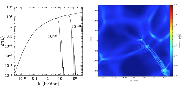
Figure 1: Left panel: the dimensionless linear mass power spectrum $\Delta^{2}(k)\equiv 4\pi k^{3}P(k)/(2\pi)^{3}$, where $P(k$) is the dimensionful version, as a function of comoving momentum $k$. This is the linear power spectrum at redshift $z=0$. The top curve corresponds to that of conventional cold dark matter. The other two are for wave dark matter with $m=10^{-20}$ eV and $10^{-22}$ eV respectively, exhibiting the suppression of power on small scales (high $k$’s). The transfer function is taken from Hu et al. (2000). Right panel: a $z=5$ snapshot of the dark matter density in a cosmological simulation of ultra-light dark matter with $m=10^{-22}$ eV. The snapshot is $700$ kpc comoving on a side. The color scale reflects the density (in ${\rm\,g/cm^{3}}$). Wave interference fringes can be seen along filaments and in/around halos. Such interference patterns were first seen in simulations by Schive, Chiueh & Broadhurst (2014a). Snapshot produced by Xinyu Li (Li et al., 2019).

4.3 Numerical simulations

Great strides have been made in numerical simulations of structure formation with wave dark matter (the Schrödinger-Poisson system), starting with the work of Schive, Chiueh & Broadhurst (2014a). There are by now a number of different algorithms, including spectral method and finite difference (Schive et al., 2014a, Schwabe et al., 2016, Mocz et al., 2017, Du et al., 2018b, Li et al., 2019, Edwards et al., 2018, Mocz et al., 2019, Schwabe et al., 2020), often with adaptive mesh refinement. One key challenge to solving the Schrödinger-Poisson system (Equations 12 and 13) is the high demand for resolution. In cosmological applications, one is often interested in predictions on large scales, say length scale $\lambda$. To accurately describe bulk motion on such large scales, say velocity $v$, one must include waves with the corresponding wavelength $2\pi/(mv)$. The trouble is that one is often in situations where $2\pi/(mv)\ll\lambda$. For instance, with $m\sim 10^{-22}$ eV and a velocity of $100$ km/s, the de Broglie wavelength $2\pi/(mv)\sim 1.2$ kpc is a lot smaller than typical length scales of interest in large scale structure $\lambda>1$ Mpc. A wave simulation, unlike an N-body simulation, thus must have high resolution even if one is only interested in large scales. This is why existing wave simulations are typically limited to small box sizes. A related challenge is the requisite time-step: dimensional analysis applied to the Schrödinger equation tells us the time-step scales as $m\times{\,\rm resolution}^{2}$, i.e. the time-step has to be less than the de Broglie wavelength divided by the typical velocity. Contrast this with the requirement for an N-body simulation—a time step of $\,\lower 3.22916pt\hbox{$\sim$}\hbox to0.0pt{\hss\raise 1.1625pt\hbox{$<$}}\,\lambda/v$ suffices. A recent $\sim 10$ Mpc box, de-Broglie-scale-resolved, wave simulation was described by May & Springel (2021).

An alternative is to simulate the fluid formulation, expressed in Equations 13, 15 and 16 (Mocz & Succi, 2015, Veltmaat & Niemeyer, 2016, Nori & Baldi, 2018, Nori et al., 2019). With $\rho$ and $\vec{v}$ as variables (related to the amplitude and phase of $\psi$), there is no need to have high spatial resolution just to correctly capture the large scale flows. The downside is that the fluid formulation is ill-defined at places where $\rho=0$. This can be seen by looking at the form of the quantum pressure term in the Euler equation (16), or more simply, by noting that the phase of the wavefunction $\psi$ (which determines $\vec{v}$) becomes ill-defined at locations where $\rho=m|\psi|^{2}$ vanishes. One might think occurrences of vanishing $\rho$ must be rare and have a negligible impact; this turns out to be false (Li et al., 2019, Hui et al., 2020)—we will have more to say about this in Section 4.4. A promising approach to overcome this and the resolution challenge is a hybrid scheme, where the large scale evolution proceeds according to the fluid formulation or an N-body code (the vanishing-$\rho$ issue does not arise on large scales), and the small scale evolution follows the wave formulation (Veltmaat et al., 2018).

Recall that the Schrödinger equation originates as a non-relativistic approximation to the Klein-Gordon equation. If one is interested in applications where relativity plays a role, such as a soliton close to its maximum possible mass (Section 4.2), or the scalar field close to black holes or in the early universe, a Klein-Gordon code (or more generally, a code to evolve a scalar with arbitrary potential) should be used. There are many examples in the literature: Felder & Tkachev (2008), Easther et al. (2009), Giblin et al. (2010), Amin et al. (2012), Helfer et al. (2017), Widdicombe et al. (2018), Buschmann et al. (2020), Eggemeier & Niemeyer (2019).

Much of the recent progress in understanding halo substructure for wave dark matter comes from numerical simulations, often in the ultra-light regime of $m\sim 10^{-22}$ eV. Many of the qualitative features carry over to higher masses; the quantitative implications for observations/experiments are mass specific of course, as we will discuss.

4.4 Wave interference—granules and vortices

The right panel of Figure 1 shows the dark matter density in a snapshot of a cosmological wave simulation (Li et al., 2019). A striking feature is the presence of interference fringes, a characteristic prediction of wave dark matter, first demonstrated in cosmological simulations by Schive, Chiueh & Broadhurst (2014a), and subsequently confirmed by many groups (Schive et al., 2014a, Schwabe et al., 2016, Veltmaat & Niemeyer, 2016, Mocz et al., 2017, Du et al., 2018b, Li et al., 2019, Edwards et al., 2018, Nori & Baldi, 2018, Veltmaat et al., 2018, Mocz et al., 2019, Schwabe et al., 2020). The interference patterns are particularly obvious in the nonlinear regime, along filaments and in/around collapsed halos. In these nonlinear objects, wave interference causes order one fluctuations in density: blobs of constructive interference of de Broglie size (sometimes called granules) interspersed between patches of destructive interference.

As a simple model of a galactic halo, consider a superposition of plane waves:

$$\psi(t,\vec{x})=\sum_{\vec{k}}A_{\vec{k}}e^{iB_{\vec{k}}}e^{i{\vec{k}}\cdot{\vec{x}}-i\omega_{k}t}\,,$$ (25)

where $A_{\vec{k}}$ and $B_{\vec{k}}$ are the amplitude and phase of each plane wave of momentum $\vec{k}$. In a virialized halo, it is reasonable to expect, as a zero order approximation, that the phases $B_{\vec{k}}$’s are randomly distributed. This is the analog of assuming random orbital phases for stars in a halo. We refer to this as the random phase halo model. The amplitudes $A_{\vec{k}}$’s should reflect the velocity (or momentum) dispersion within the halo. For instance we can adopt $A_{\vec{k}}\propto e^{-k^{2}/k_{0}^{2}}$ (where $k=|\vec{k}|$), resembling an isothermal distribution, with a de Broglie wavelength $\propto 1/k_{0}$. The density is:

$$\rho=m|\psi|^{2}=m\sum_{\vec{k}}A_{\vec{k}}^{2}+m\sum_{\vec{k}\neq\vec{k}^{\prime}}A_{\vec{k}}A_{\vec{k}^{\prime}}e^{i(B_{\vec{k}}-B_{\vec{k}^{\prime}})}e^{i({\vec{k}}-{\vec{k}^{\prime}})\cdot\vec{x}-i(\omega_{k}-\omega_{k^{\prime}})t}\,.$$ (26)

The first term comes from squaring each Fourier mode and summing them. The second represents the contribution from interference between different Fourier modes. It is the second term that is responsible for the appearance of interference fringes in numerical simulations such as shown in Figure 1. The typical difference in momenta between different Fourier modes is of the order of $k_{0}$, which fixes the characteristic size of the interference fringes or granules i.e. the de Broglie wavelength $\sim 2\pi/k_{0}$. The typical difference in energy between the modes is of the order of $\sim k_{0}^{2}/(2m)\sim k_{0}v/2$, where $v$ is the velocity dispersion. This determines the characteristic time scale over which the interference pattern changes i.e. the de Broglie time:

$$t_{\rm dB}\equiv{2\pi\over mv^{2}}=1.9\times 10^{6}{\,\rm yr.}\left({10^{-22}{\,\rm eV}\over m}\right)\left({250{\,\rm km/s}\over v}\right)^{2}$$

$$\quad=5.9\times 10^{-3}{\,\rm s}\left({10^{-6}{\,\rm eV}\over m}\right)\left({250{\,\rm km/s}\over v}\right)^{2}\,.$$ (27)

There is some arbitrariness in the choice of the prefactor $2\pi$. Reasonable choices range within factor of a few.

In other words, wave interference produces de-Broglie-scale, order unity density fluctuations which vary on time scale of $t_{\rm dB}$. Such fluctuations can in principle take the density all the way to zero i.e. complete destructive interference. What is interesting is that (1) such occurrences are not rare, and (2) the locations of complete destructive interference are vortices. This was explored in Chiueh et al. (2011), Hui et al. (2020). Below we summarize the findings, following the line of reasoning in Hui et al. (2020).

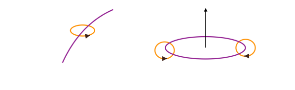
Figure 2: Schematic illustration of vortices. Left panel: a vortex line, or segment thereof (purple line). The loop with arrow indicates velocity circulation (or phase winding) around the vortex. Right panel: a vortex ring (purple line). The loops with arrows indicate velocity circulation. The arrow in the middle indicates the bulk motion of the ring.

In three spatial dimensions, the set of points where the real part of the wavefunction vanishes generically forms a surface. Likewise for the imaginary part. Demanding both parts of the wavefunction vanish thus gives a line, where the two surfaces cross. The purple line in the left panel of Figure 2 depicts such a line of vanishing $\psi$ (i.e. the amplitude of $\psi$ is zero and the phase is ill-defined on the line). Consider a loop going around this line: for the wavefunction to be single-valued, the phase of the wavefunction must wind by integers of $2\pi$. Recall the fluid velocity is given by the gradient of the phase (Equation 14); integrating the velocity around a loop encircling the line of vanishing $\psi$ gives:

$${\rm circulation\,}\equiv\oint d\vec{x}\cdot\vec{v}={2\pi n\over m}\,,$$ (28)

where $n$ is an integer. The line of vanishing $\psi$ is therefore a vortex. It is helpful to consider a Taylor expansion around a point on the vortex (let’s take it to be the origin):

$$\psi(\vec{x})\sim\vec{x}\,\cdot\vec{\nabla}\psi|_{0}\,,$$ (29)

assuming $\vec{\nabla}\psi|_{0}$, the derivative evaluated at $x=0$, does not vanish. It can be shown the winding number $n=\pm 1$ as long as $\vec{\nabla}\psi|_{0}$ does not vanish. If it vanishes, one would have to consider the next higher order term in the Taylor expansion, yielding higher winding. A vortex line, much like a magnetic field line, cannot end, and so one expects generically a vortex ring, depicted in the right panel of Figure 2. It can be further shown that, in addition to velocity circulation around the ring, the ring itself moves with a bulk velocity that scales inversely with its size. Analytic solutions illustrating this behavior (and more) can be found in Bialynicki-Birula et al. (2000), Hui et al. (2020).

A number of features of vortices in wave dark matter are worth stressing. (1) One might think these locations of chance, complete destructive interference must be rare, but they are actually ubiquitous: on average there is about one vortex ring per de Broglie volume in a virialized halo. This has been verified analytically in the random phase halo model, and in numerical wave simulations of halos that form from gravitational collapse. Note that gravity plays an important role in the formation of vortices in the cosmology setting. In the early universe, the density (and the wavefunction) is roughly homogeneous with very small fluctuations; this means nowhere does the wavefunction vanish. It is only after gravity amplifies the density fluctuations, to order unity or larger, is complete destructive interference possible. (2) Vortex rings in a realistic halo are not nice round circles, but rather deformed loops. Nonetheless, certain features are robust. Close to a vortex, the velocity scales as $1/r$ where $r$ is distance from vortex (following from Equation 28), and the density scales as $r^{2}$ (following from Equation 29). Moreover, a segment of a ring moves with a velocity that scales with the curvature i.e. curvier means faster. (3) Vortex rings come in a whole range of sizes: the distribution is roughly flat below the de Broglie wavelength, but is exponentially suppressed beyond that. (4) Vortex rings are transient, in the same sense that wave interference patterns are. The coherence time is roughly the de Broglie time (Equation 4.4). Vortex rings cannot appear or disappear in an arbitrary way, though. A vortex ring can appear by first nucleating as a point, and then growing to some finite size. It can disappear only by shrinking back to a point (or merge with another ring). This behavior can be understood as a result of Kelvin’s theorem: recall that the fluid description is valid away from vortices; conservation of circulation tells us that vortices cannot be arbitrarily removed or created.

To summarize, wave interference substructures, of which vortices are a dramatic manifestation, are a unique signature of wave dark matter. It is worth stressing that while the wave nature of dark matter leads to a suppression of small scale power in the linear regime (Section 4.1), it leads to the opposite effect in the nonlinear regime, by virtue of interference. We discuss the implications for observations and experiments in Section 5.

4.5 Dynamical processes—relaxation, oscillation, evaporation, friction and heating

An interesting phenomenon in a wave dark matter halo is soliton condensation, first pointed out by Schive et al. (2014a, b). It is observed that virialized halos in a cosmological simulation tend to have a core that resembles the soliton discussed in Section 4.2, with a soliton mass that scales with the halo mass as:

$$M_{\rm soliton}\sim 6.7\times 10^{7}{\,\rm M_{\odot}}{10^{-22}{\,\rm eV}\over m}\left({M_{\rm halo}\over 10^{10}{\,\rm M_{\odot}}}\right)^{1/3}\,.$$ (30)

The condensation process was studied by solving the Landau kinetic equation in Levkov et al. (2018) (see also Seidel & Suen, 1994, Harrison et al., 2003, Guzman & Urena-Lopez, 2006b, Schwabe et al., 2016). Here, we describe a heuristic derivation of the condensation, or relaxation, time scale (Hui et al., 2017). Consider the part of a halo interior to radius $R$, with velocity dispersion $v$. Suppose there is no soliton yet. Wave interference as described in Section 4.4 inevitably produces granules of de Broglie size $\lambda_{\rm dB}$. In this region, we have $\sim(2R/\lambda_{\rm dB})^{3}$ such granules or quasi-particles. The relaxation time for such a gravitational system is roughly a tenth of the crossing time $2R/v$ times the number of granules i.e.

$$t_{\rm relax}\sim 0.1{2R\over v}\left({2R\over\lambda_{\rm dB}}\right)^{3}\sim 10^{8}{\,\rm yr}\left({R\over 2{\,\rm kpc}}\right)^{4}\left({v\over 100{\,\rm km/s}}\right)^{2}\left({m\over 10^{-22}{\,\rm eV}}\right)^{3}$$

$$\sim 10^{8}{\,\rm yr}\left({0.14{\,\rm M_{\odot}}/{\,\rm pc}^{3}\over\rho}\right)^{2}\left({v\over 100{\,\rm km/s}}\right)^{6}\left({m\over 10^{-22}{\,\rm eV}}\right)^{3}\,.$$ (31)

In essence, we have adapted the standard relaxation time for a gravitational system (Binney & Tremaine, 2008) by replacing the number of particles/stars by the number of de Broglie granules. The above estimate suggests the condensation of solitons quickly becomes inefficient for larger values of $m$. It remains to be verified, though, whether this is indeed the relevant time scale for soliton formation in a cosmological setting where halos undergo repeated mergers. For instance, in a numerical study of six halos by Veltmaat et al. (2018), all halos have substantial cores from the moment of halo formation, though two of them exhibit some core growth over time.

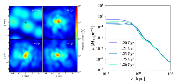
Figure 3: Left panel: Snapshots of the formation of a halo. Clockwise from top-left: initial moment, $1$ Gyr, $1.2$ Gyr and $1.1$ Gyr. Each snapshot is $10$ kpc on a side. Color coding denotes the projected density in ${\rm M_{\odot}/\,\rm pc^{2}}$. The cross in the middle denotes the center of mass. Note how the soliton core wanders. Right panel: Spherically averaged density profile (density in ${\rm M_{\odot}/\,\rm pc}^{3}$ as a function of radius in kpc) at several different moments, from $1.2$ Gyr to $1.26$ Gyr. The soliton core exhibits persistent oscillations. Soliton oscillations and random walk were first observed in simulations by Veltmaat et al. (2018), Schive et al. (2020). Figure adapted from Li et al. (2021).

Detailed studies of simulations suggest the core of a fuzzy dark matter halo is not an exact soliton. Veltmaat, Niemeyer & Schwabe (2018) pointed out that the core object has persistent oscillations, and Schive, Chiueh & Broadhurst (2020) demonstrated that it random walks (see Figure 3). This is another manifestation of wave interference. Think of the halo gravitational potential as approximately constant (in time); the halo can be decomposed into a superposition of energy eigenstates (Lin et al., 2018). The ground state (i.e. the solitonic state) contributes substantially to the density around the halo center, but it is not the only state that does. Interference between the ground state and excited states approximately matches the core oscillations and random walk observed in simulations (Li et al., 2021, Padmanabhan, 2021).

It is well known that a subhalo embedded inside a larger parent halo can be tidally disrupted. The tidal radius is roughly where the average interior density of the subhalo matches that of the parent halo. Quantum pressure adds a new twist to this story: even mass within the tidal radius of the subhalo is unstable to disruption. The evaporation time scale of a soliton inside a host halo was computed in Hui et al. (2017): a soliton would evaporate in $\,\lower 3.22916pt\hbox{$\sim$}\hbox to0.0pt{\hss\raise 1.1625pt\hbox{$<$}}\,10$ orbits if its density is $\,\lower 3.22916pt\hbox{$\sim$}\hbox to0.0pt{\hss\raise 1.1625pt\hbox{$<$}}\,60$ times the host density. This was verified in wave simulations by Du et al. (2018b).

The wave nature of dark matter also has an impact on dynamical friction. Recall how dynamical friction works: a heavy object ploughs through a sea of dark matter particles; gravitational scattering creates an overdense tail of particles in its wake; the overdense tail gravitationally pulls on the heavy object, effecting friction. For wave dark matter, one expects a smoothing of the overdense tail on the de Broglie scale. The dynamical friction is thus suppressed. A computation, neglecting self-gravity of the dark matter and assuming the unperturbed background is homogenous, is described in Hui et al. (2017) (see also Lora et al., 2012): while the frictional force is $4\pi\rho(GM/v)^{2}\left({\,\rm ln}[2r/(GM/v^{2})]-1\right)$ in the particle limit, it is $4\pi\rho(GM/v)^{2}\left({\,\rm ln}[2rmv]-1+\gamma\right)$ in the wave limit. Here, $\rho$ is the background mass density, $M$ is the mass of the heavy object (such as a globular cluster), $v$ is the velocity of the heavy object, $r$ is the size of the galactic halo or the orbital radius of $M$ in the halo, and $\gamma=0.577...$ is the Euler-Mascheroni constant. The distinction between the particle limit (i.e. Chandrasekhar) and the wave limit comes down to comparing two length scales: $GM/v^{2}$ (the impact parameter at which significant deflection occurs) versus the de Broglie scale $\sim 1/(mv)$. The wave limit applies when the former is less than the latter i.e. if the following ratio is small:

$${GM/v^{2}\over(1/mv)}=0.002\left({M\over 10^{6}{\,\rm M_{\odot}}}\right)\left({100{\rm\,km/s}\over v}\right)\left({m\over 10^{-22}{\,\rm eV}}\right)\,.$$ (32)

Depending on the parameters of interest, dynamical friction can be suppressed significantly, if $m$ is in the ultra-light range. A computation of dynamical friction in more general fluid dark matter is carried out in Berezhiani et al. (2019). Investigations of dynamical friction in fuzzy dark matter in more realistic settings— inhomogeneous background, with de Broglie granules—can be found in Du et al. (2017), Bar-Or et al. (2019), Lancaster et al. (2020).

We close this section with a discussion of one more dynamical effect from the wave nature of dark matter. Recall from Section 4.4 that the wave interference pattern of granules and vortices is transient, on time scale of $t_{\rm dB}$ (Equation 4.4). The fluctuating gravitational potential leads to the heating and scattering of stars (Hui et al., 2017, Amorisco & Loeb, 2018, Bar-Or et al., 2019, Church et al., 2019, Marsh & Niemeyer, 2019, Schive et al., 2020). A rough estimate can be obtained as follows. Consider a star undergoing deflection by a de Broglie blob: the angle of (weak) deflection is $\sim 2GM/(bv^{2})$ where $M$ is the mass of the blob and $b$ is the impact parameter. The deflection imparts a kick to the velocity of the star, perpendicular to the original direction of motion: $\Delta v\sim 2GM/(bv)$. Using $M\sim 4\pi\rho(\lambda_{\rm dB}/2)^{3}/3$ and $b\sim\lambda_{\rm dB}/2$, one finds

$$\Delta v\sim 0.08{\,\rm km/s}\left({\rho\over 0.01{\,\rm M_{\odot}\,pc^{-3}}}\right)\left({250{\,\rm km/s}\over v}\right)^{3}\left({10^{-22}{\,\rm eV}\over m}\right)^{2}\,.$$ (33)

This is a stochastic kick, and its rms value accumulates in a root $N$ fashion, where $N$ is the number of de Broglie blobs the star encounters, which is roughly $Tv/\lambda_{\rm dB}$ where $T$ is the time over which such encounters take place. Thus,

$${\rm rms\,}\Delta v\sim 4{\,\rm km/s}\left({T\over 5{\,\rm Gyr}}\right)^{1/2}\left({\rho\over 0.01{\,\rm M_{\odot}\,pc^{-3}}}\right)\left({250{\,\rm km/s}\over v}\right)^{2}\left({10^{-22}{\,\rm eV}\over m}\right)^{3/2}\,.$$ (34)

See Bar-Or et al. (2019), Church et al. (2019) for more careful analyses of such heating. We discuss the implications for tidal streams, galactic disks and stellar clusters in Section 5.

4.6 Compact objects and relativistic effects—black hole accretion, superradiance and potential oscillation

What happens to wave dark matter around compact objects, such as black holes? First of all, accretion onto black holes should occur. This includes accretion of both mass and angular momentum. Second, for a spinning black hole, the reverse can happen: mass and angular momentum can be extracted out of a Kerr black hole, an effect known as superradiance.

To study these phenomena properly, because relativistic effects become relevant close to the horizon, one needs to revert to the Klein-Gordon description i.e. $\phi$ obeying Equation 10. There is a long history of studying solutions to the Klein-Gordon equation in a Schwarzschild or Kerr background (Starobinskiǐ, 1973, Unruh, 1976, Detweiler, 1980, Bezerra et al., 2014, Vieira et al., 2014, Konoplya & Zhidenko, 2006, Dolan, 2007, Arvanitaki et al., 2010, Arvanitaki & Dubovsky, 2011, Barranco et al., 2012, Arvanitaki et al., 2017). The treatments generally differ in the boundary conditions assumed: while the boundary condition at the horizon is always ingoing, that far away can be outgoing (for studying quasi-normal modes), asymptotically vanishing (for studying superradiance clouds), or infalling (for studying accretion), or combination of infalling and outgoing (for studying scattering).

For a black hole immersed in a wave dark matter halo, the infalling boundary condition is the most relevant. In particular, the stationary accretion flow around a black hole was investigated in Clough et al. (2019), Hui et al. (2019), Bamber et al. (2020) i.e. the time-dependence of $\phi$ is a linear combination of $e^{\pm imt}$ at all radii. The Klein-Gordon equation in a Schwarzschild background takes the form:

$$\left[\partial_{t}^{2}-\partial_{r_{*}}^{2}+U(r)\right](r\phi)=0\quad,\quad U(r)\equiv\left(1-{r_{s}\over r}\right)\left(m^{2}+{\ell(\ell+1)\over r^{2}}+{r_{s}\over r^{3}}\right)\,,$$ (35)

where $t$ and $r$ are the time and radial coordinates of the Schwarzschild metric, $r_{s}$ is the Schwarzschild radius, and $r_{*}$ is the tortoise coordinate: $r_{*}=r+r_{s}{\,\rm log\,}(r/r_{s}-1)$. We have assumed the angular dependence of $\phi$ is given by a spherical harmonic of some $\ell$. For $\phi\propto e^{\pm imt}$, this resembles the Schrödinger equation with some potential. For $\ell=0$, the radial profile of $\phi$ goes roughly as follows: (1) for $r_{s}^{-1}\,\lower 3.22916pt\hbox{$\sim$}\hbox to0.0pt{\hss\raise 1.1625pt\hbox{$<$}}\,m$, we have $\phi\sim r^{-3/4}$ i.e. there is a pile-up of the scalar towards the horizon; (2) for $m\,\lower 3.22916pt\hbox{$\sim$}\hbox to0.0pt{\hss\raise 1.1625pt\hbox{$<$}}\,v_{\rm halo}\,r_{s}^{-1}$, where $v_{\rm halo}$ is the velocity dispersion of the ambient halo, the scalar profile is more or less flat; (3) for $m$ in between these two limits, $\phi$ exhibits both particle behavior (the $r^{-3/4}$ pile-up) and wave behavior in the form of standing waves. The computation described above assumes the black hole dominates gravitationally: one can check that, for astrophysically relevant parameters, the pile-up of the scalar towards the horizon does not lead to significant gravitational backreaction. There is, however, the possibility that self-interaction (the quartic interaction for the axion) might be non-negligible close to the horizon due to the pile-up. As one goes to larger distances from the black hole, the dark matter (and baryons) eventually dominates gravitationally. An interesting setting is the wave dark matter soliton at the center of a galaxy which also hosts a supermassive black hole (Brax et al., 2020). Investigations of how the black hole modifies the soliton can be found in Chavanis (2019), Bar et al. (2019b), Davies & Mocz (2020).

Even though the instantaneous gravitational backreaction of the scalar is small close to the black hole, the cumulative accreted mass could be significant. The accretion rate in the low $m$ regime (for $\ell=0$) is:

$$\dot{M}_{\rm BH}=4\pi r_{s}^{2}\rho_{\rm halo}\sim 4\times 10^{-9}{\,\rm M_{\odot}}{\,\rm yr}^{-1}\left({M_{\rm BH}\over 10^{9}{\,\rm M_{\odot}}}\right)^{2}\left({\rho_{\rm halo}\over 0.1{\,\rm M_{\odot}\,pc^{-3}}}\right)$$ (36)

where $M_{\rm BH}$ is the mass of the black hole, and $\rho_{\rm halo}$ is the ambient dark matter halo density. In the high $m$ regime, the pile-up enhances this by a factor of $\sim 1/v_{\rm halo}^{3}$. For $v_{\rm halo}\sim 10^{-3}$, we see that $\dot{M}_{\rm BH}$ goes up to $4{\,\rm M_{\odot}/yr}$ in the high $m$ limit, though it should be kept in mind this estimate assumes $\ell=0$. (Note that $r_{s}^{-1}=6.7\times 10^{-20}{\,\rm eV}(10^{9}{\,\rm M_{\odot}\,}/M_{\rm BH})$.)

Suppose one solves the Klein-Gordon equation with a different boundary condition far away from the black hole: that $\phi$ vanishes. In that case, assuming the time dependence is given by $e^{-i\omega t}$, the allowed frequency $\omega$ forms a discrete spectrum, much like the energy spectrum of a hydrogen atom. For a spinning black hole, some of these $\omega$’s are complex with a positive imaginary part, signaling an instability, known as superradiance (Zel’Dovich, 1972, Bardeen et al., 1972, Press & Teukolsky, 1972, Starobinskiǐ, 1973, Damour et al., 1976, Dolan, 2007, Arvanitaki et al., 2010, Arvanitaki & Dubovsky, 2011, Arvanitaki et al., 2017, Endlich & Penco, 2017). The superradiance condition is:

$${\,\rm Re\,}\omega<{am_{J}\over{r_{s}r_{+}}}$$ (37)

where $r_{s}=2GM$, $r_{+}=(r_{s}/2)+\sqrt{(r_{s}/2)^{2}-a^{2}}$ is the horizon, $a$ is the black hole angular momentum per unit mass (the dimensionless spin is $2a/r_{s}$, between $0$ and $1$), and $m_{J}$ is the angular momentum quantum number of the mode in question. A superradiant mode extracts energy and angular momentum from the black hole. That this mode grows with time means the scalar need not be dark matter at all— even quantum fluctuations could provide the initial seed to grow a whole superradiance cloud around the black hole. In the process, the black hole loses mass and angular momentum (much of which occurs when the cloud is big). At some point, the black hole’s mass and spin are such that the mode in question is no longer unstable, and in fact some of the lost energy and angular momentum flow back into the black hole, until another superradiant mode—one that grows more slowly, typically higher $\ell$—takes over (see e.g. Ficarra et al., 2019). The implied net black hole spin-down is used to put constraints on the existence of light scalars, using black holes with spin measurements (for recent discussions, see e.g. Stott & Marsh, 2018, Davoudiasl & Denton, 2019). Other phenomena associated with the black hole superradiance cloud includes gravitational wave emission, and run-away explosion when self-interaction becomes important (Arvanitaki & Dubovsky, 2011, Yoshino & Kodama, 2014, Hannuksela et al., 2019).

It is worth stressing that these constraints do not assume the scalar in question is the dark matter. An interesting question is how the constraints might be modified if the scalar is the dark matter. For instance there can be accretion of angular momentum from the ambient dark matter, much like the accretion of mass discussed earlier. The cloud surrounding the black hole is thus a combination of superradiant unstable and stable modes. This was explored in Ficarra et al. (2019): if the initial seed cloud (of both unstable and stable modes) is large enough, the long term evolution of the black hole mass and spin can be quite different from the case of a small initial seed. This is particularly relevant if the scalar in question is the dark matter, and therefore present around the black hole from the beginning. It would be worth quantifying how existing superradiance constraints might be modified in this case. There are also interesting investigations on how such a cloud interacts with a binary system (Baumann et al., 2019, Zhang & Yang, 2020, Annulli et al., 2020).

We close this section with the discussion of one more relativistic effect, pointed out by Khmelnitsky & Rubakov (2014). The energy density associated with the oscillations of $\phi$ (which can be interpreted as a collection of $\phi$ particles) is $\rho=(\dot{\phi}^{2}+m^{2}\phi^{2})/2$ (Equation 7). It can be shown the corresponding pressure is $P=(\dot{\phi}^{2}-m^{2}\phi^{2})/2$. For $\phi\sim{\,\rm sin}(mt)$ or ${\,\rm cos}(mt)$, we see that $\rho$ is constant while $P$ oscillates with frequency $2m$. Einstein equations tell us this sources an oscillating gravitational potential. In Newtonian gauge, with the spatial part of the metric as $g_{ij}=(1-2\Psi)\delta_{ij}$, the gravitational potential $\Psi$ has a constant piece that obeys the usual Poisson equation $\nabla^{2}\Psi=4\pi G\rho$, and an oscillating part obeying $-\ddot{\Psi}\sim 4\pi GP$. Thus $\Psi$ oscillates with frequency $2m$ and amplitude $\pi G\rho/m^{2}$. In other words, the oscillating part of $\Psi$ is suppressed compared to the constant part by $k^{2}/m^{2}$. The typical (constant part of) gravitational potential is of the order $10^{-6}$ in the Milky Way; the oscillating part is then about $10^{-12}$. For $m$ in the ultra-light range, recalling $m^{-1}\sim 0.2{\,\rm yr}\,(10^{-22}{\,\rm eV}/m)$, pulsar timing arrays are well suited to search for this effect, as proposed by Khmelnitsky & Rubakov (2014). See further discussions in Section 5.4.

5 Observational/experimental implications and constraints

In this section, we discuss the observational and experimental implications of the wave dynamics and phenomenology explained above. The discussion serves a dual function. One is to summarize current constraints—because of the wide scope, the treatment is more schematic than in previous sections, but provides entry into the literature. The other is to point out the limitations of current constraints, how they might be improved, and to highlight promising new directions. Astrophysical observations are relevant mostly, though not exclusively, for the ultra-light end of the spectrum. Axion detection experiments, on the other hand, largely probe the heavier masses, though new experiments are rapidly expanding the mass range. Much of the discussion applies to any wave dark matter candidate whose dominant interaction is gravitational. Some of it—on axion detection experiments for instance— applies specifically to axions with their expected non-gravitational interactions (Equation 9).

Sections 5.2 and 5.3 focus on ultra-light wave dark matter i.e. fuzzy dark matter. Table 1 summarizes some of the corresponding astrophysical constraints. Sections 5.1, 5.4, 5.5 and 5.6 cover more general wave dark matter, with Section 5.6 on axion detection experiments.

5.1 Early universe considerations

Within the inflation paradigm, the light scalar $\phi$ associated with wave dark matter has inevitable quantum fluctuations which are stretched to large scales by an early period of accelerated expansion (Axenides et al., 1983, Linde, 1985, Seckel & Turner, 1985, Turner & Wilczek, 1991). These are isocurvature fluctuations, distinct from the usual adiabatic fluctuations associated with the inflaton $\varphi$, which is another light scalar. The relevant power spectra are (e.g., Baumann, 2011, Marsh et al., 2013):

$$\Delta_{\zeta}^{2}={1\over 8\pi^{2}\epsilon}{H_{\rm infl}^{2}\over m_{\rm pl}^{2}}\quad,\quad\Delta_{\phi}^{2}={1\over\pi^{2}}{H_{\rm infl}^{2}\over\phi_{i}^{2}}\,,$$ (38)

where $\Delta_{\zeta}^{2}$ is the (adiabatic) curvature power spectrum, $\Delta_{\phi}^{2}$ is the (isocurvature) density power spectrum for $\phi$, $H_{\rm infl}$ is the Hubble scale during inflation, $m_{\rm pl}\equiv 1/\sqrt{8\pi G}\sim 2.4\times 10^{18}{\,\rm GeV}$ is the reduced Planck mass, $\phi_{i}$ is the (axion) scalar field value during inflation, and $\epsilon$ is the first slow-roll parameter. Microwave background anisotropies bound $\Delta_{\phi}^{2}/\Delta_{\zeta}^{2}\,\lower 3.22916pt\hbox{$\sim$}\hbox to0.0pt{\hss\raise 1.1625pt\hbox{$<$}}\,0.05$ (Hinshaw et al., 2013, Aghanim et al., 2020), implying $8\epsilon(m_{\rm pl}/\phi_{i})^{2}\,\lower 3.22916pt\hbox{$\sim$}\hbox to0.0pt{\hss\raise 1.1625pt\hbox{$<$}}\,0.05$. Consider for instance $\phi_{i}\sim 10^{17}$ GeV (see Equation 8, where $\phi_{i}\sim f$). In that case, observations require $\epsilon\,\lower 3.22916pt\hbox{$\sim$}\hbox to0.0pt{\hss\raise 1.1625pt\hbox{$<$}}\,10^{-5}$. Since $\Delta^{2}_{\zeta}$ is observed to be about $10^{-9}$, this implies $H_{\rm infl}/m_{\rm pl}\,\lower 3.22916pt\hbox{$\sim$}\hbox to0.0pt{\hss\raise 1.1625pt\hbox{$<$}}\,10^{-6}$. This is a low inflation scale, suggesting a low level of gravitational waves, or tensor modes (Lyth, 1990). One can see this more directly by recalling that tensor modes suffer the same level of fluctuations as a spectator scalar like $\phi$:

$$\Delta^{2}_{\rm tensor}={2\over\pi^{2}}{H_{\rm infl}^{2}\over m_{\rm pl^{2}}}\quad,\quad r\equiv{\Delta^{2}_{\rm tensor}\over\Delta^{2}_{\zeta}}=16\epsilon$$ (39)

where $\Delta_{\rm tensor}^{2}$ resembles $\Delta_{\phi}^{2}$, with $\phi_{i}$ replaced by $m_{\rm pl}$, and a factor of $2$ for the $2$ polarizations. The tensor-to-scalar ratio $r$ is thus constrained by the isocurvature bound to be: $r\,\lower 3.22916pt\hbox{$\sim$}\hbox to0.0pt{\hss\raise 1.1625pt\hbox{$<$}}\,0.1(\phi_{i}/m_{\rm pl})^{2}$. For $\phi_{i}\sim 10^{17}$ GeV, this means $r\,\lower 3.22916pt\hbox{$\sim$}\hbox to0.0pt{\hss\raise 1.1625pt\hbox{$<$}}\,2\times 10^{-4}$, making tensor modes challenging to observe with future microwave background experiments. Most axion models have lower $\phi_{i}$’s which would strengthen the bound. This is thus a general requirement: to satisfy the existing isocurvature bound, the inflation scale $H_{\rm infl}$ must be sufficiently low, implying a low primordial gravitational wave background. This holds as long as the scalar dark matter derives its abundance from the misalignment mechanism, with the misalignment angle in place during inflation. A way to get around this is to consider models where the scalar $\phi$ becomes heavy during inflation (Higaki et al., 2014).

The requirement does not apply in cases where the relic abundance is determined by other means. For instance, for the QCD axion, it could happen that the Peccei-Quinn symmetry is broken only after inflation (recall the axion as a Goldstone mode exists only after spontaneous breaking of the symmetry), in which case the relic abundance is determined by the decay of axion strings and domain walls (Kolb & Turner, 1990, Buschmann et al., 2020, Gorghetto et al., 2020). There are also proposals for vector, as opposed to scalar, wave dark matter: isocurvature vector perturbations are relatively harmless because they decay (Graham et al., 2016b, Kolb & Long, 2020).

The above discussion includes only the gravitational interaction of scalar dark matter. Other early universe effects are possible with non-gravitational interactions. For instance, Sibiryakov et al. (2020) pointed out if the scalar has a dilaton-like coupling to the standard model, Helium-4 abundance from big bang nucleosynthesis can be significantly altered.

5.2 Linear power spectrum and early structure formation

As discussed in Section 4.1, light scalar dark matter—produced out of a transition process from slow-roll to oscillations—has a primordial power spectrum suppressed on small scales (high $k$’s). For fuzzy dark matter, the suppression scale is around $k\sim 5$/Mpc (Equation 20). Observations of the Lyman-alpha forest are sensitive to power on such scales. The Lyman-alpha forest is the part of the spectrum of a distant object (usually a quasar) between Lyman-alpha and Lyman-beta in its rest frame. Intergalactic neutral hydrogen causes absorption, with measurable spatial fluctuations. With suitable modeling, the spatial fluctuations can be turned into statements about the dark matter power spectrum (Croft et al., 1998, Hui, 1999, McDonald et al., 2005b, Palanque-Delabrouille et al., 2013). With this technique, a limit of $m\,\lower 3.22916pt\hbox{$\sim$}\hbox to0.0pt{\hss\raise 1.1625pt\hbox{$>$}}\,3\times 10^{-21}$ eV was obtained by Iršič et al. (2017), Kobayashi et al. (2017), Armengaud et al. (2017). Rogers & Peiris (2020) found a stronger bound of $2\times 10^{-20}$ eV—among the differences in analysis are assumptions on the reionization history.

In this type of investigation, often the only effect of fuzzy dark matter accounted for is its impact on the primordial power spectrum. One might worry about the effect of quantum pressure on the subsequent dynamics, but this was shown to be a small effect at the scales and redshifts for the Lyman-alpha forest (Nori et al., 2019, Li et al., 2019). Another assumption is that the observed fluctuations in neutral hydrogen reflect fluctuations in the dark matter. This need not be true, since astrophysical fluctuations modulate the neutral hydrogen distribution, such as fluctuations in the ionizing background (Croft, 2004, McDonald et al., 2005a, D’Aloisio et al., 2018), the temperature-density relation (Hui & Gnedin, 1997, Cen et al., 2009, Keating et al., 2018, Wu et al., 2019, Oñorbe et al., 2019) and from galactic winds (McDonald et al., 2005a, Viel et al., 2013). Measurements of the power spectrum growth from the forest suggest the astrophysical fluctuations are sub-dominant, that gravity is sufficient to account for the observed growth (McDonald et al., 2005b). Nonetheless, it is worth stressing for the bound on $m$, one has to worry about systematic effects at the few percent level. The astrophysical fluctuations were accounted for in the following way in deriving constraints (Iršič et al., 2017, Kobayashi et al., 2017, Armengaud et al., 2017). Simulations with these astrophysical fluctuations are compared against those without; the scale and redshift dependence of the fractional difference in the predicted Lyman-alpha power spectrum is then fixed, while the amplitude of the difference is treated as a free parameter to be determined from the data. The question is to what extent simulations of the astrophysical fluctuations have enough variety to account for the range of possible scale and redshift dependence. The variety in question derives from the distribution of ionizing sources, the reionization history and the strength and form of galactic feedback.

Formation of the first nonlinear objects in the universe is also sensitive to the small scale power spectrum. Recall in hierarchical structure formation, it is the small, less massive objects that form first. A suppression of small scale power implies fewer nonlinear objects at high redshifts, delaying reionization (Barkana et al., 2001). The EDGES experiment (Bowman et al., 2018) announced the detection of an absorption feature around $78$ MHz that may result from the hyperfine transition (21cm) of hydrogen at redshift around $15-20$. This suggests the spin temperature of the 21cm line is coupled to the gas temperature at such high redshifts, and points to early star formation which produces the requisite radiation to do so. This was used to place bounds on fuzzy dark matter $m\,\lower 3.22916pt\hbox{$\sim$}\hbox to0.0pt{\hss\raise 1.1625pt\hbox{$>$}}\,5\times 10^{-21}$ eV (Safarzadeh et al., 2018, Schneider, 2018, Lidz & Hui, 2018). A few considerations should be kept in mind. The EDGES detection remains to be confirmed (Hills et al., 2018). These bounds assume (1) star formation tracking halo formation, and (2) an upper limit on the fraction of halo baryons that turn into stars ($0.05$ in Lidz & Hui, 2018). Another important assumption is that the halo mass function can be reliably predicted from the linear power spectrum by the standard Press-Schechter or Sheth-Tormen relations (Press & Schechter, 1974, Sheth & Tormen, 1999, Marsh & Silk, 2014, Kulkarni & Ostriker, 2020). These relations have been checked for fuzzy dark matter models using only N-body, as opposed to wave, simulations, i.e. the “fuzziness” enters only through the primordial power spectrum (Schive et al., 2016). Typical wave simulations use too small a box size to give a reliable halo mass function. It is conceivable that wave interference phenomena might help make more smaller objects than expected from Press-Schechter type arguments.

Looking towards the future, spectral distortion measurements of the microwave background hold the promise of measuring the linear power spectrum down to very small scales, comoving $k$ as high as $10^{4}$/Mpc (Kogut et al., 2019, Chluba et al., 2019). From Equation 20, this kind of experiment can thus probe a wave dark matter mass as high as $\sim 10^{-15}$ eV.

Table 1: Some constraints in the literature on fuzzy dark matter

Method	Constraint	Sources of systematic uncertainties	Refs.
Lyman-alpha forest	m $>3\times 10^{-21}$ eV	Ionizing background/temp. fluctuations	1
Density profile	m $>10^{-21}$ eV	Baryonic feedback/black hole	2
Satellite mass	m $>6\times 10^{-22}$ eV	Tidal stripping	3
Satellite abundance	m $>2.9\times 10^{-21}$ eV	Subhalo mass function prediction	4

References: 1=Iršič et al. (2017), Kobayashi et al. (2017), Armengaud et al. (2017), 2=Bar et al. (2018), 3=Safarzadeh & Spergel (2019), 4=Nadler et al. (2020). See text on the methodology and systematic uncertainties of each constraint.

5.3 Galactic dynamics and structure—density profile, stellar scattering, dynamical friction, subhalo mass function and interference substructures

There is a wide variety of methods to constrain wave dark matter from galactic structure or dynamics, especially at the ultra-light end of the spectrum.

Density profile. Wave simulations demonstrate that fuzzy dark matter halos generically have a solitonic core, and an NFW-like outer density profile (Schive et al., 2014b). There is a substantial literature on comparing this prediction against observations. Investigations focusing on the inner density profile (i.e. within the purported soliton) of Milky Way dwarf satellites found reasonable agreement with $m\sim 10^{-22}-10^{-21}$ eV (Chen et al., 2017, Calabrese & Spergel, 2016). A $10^{9}\,{\,\rm M_{\odot}}$ soliton at the center of the Milky Way was reported by De Martino et al. (2020), though there is substantial uncertainty because of the dominance of baryons (Li et al., 2020). Investigations bearing on how the soliton connects with the outer halo generally found tension with data, for $m\,\lower 3.22916pt\hbox{$\sim$}\hbox to0.0pt{\hss\raise 1.1625pt\hbox{$<$}}10^{-21}$ eV. Taking the soliton-halo relation (Equation 30) seriously, one expects an inner circular velocity that matches the outer asymptotic value (a reflection of the rough equality of the soliton potential and halo potential; see footnote 22), something not seen in observations of disk galaxies (Bar et al., 2018). Moreover, dynamical measurements of Milky Way dwarf satellites, when used to fit for solitonic cores, predict halo masses that are too large, incompatible with their survival under dynamical friction, giving a bound of $m\,>\,6\times 10^{-22}$ eV (Safarzadeh & Spergel, 2019). It was also pointed out by Burkert (2020) that low mass galaxies have a universal core surface density $\sim 75\,{\,\rm M_{\odot}/pc^{2}}$ while spanning a large range in core radius; this conflicts with the soliton scaling of $M\propto 1/R$ (Equation 4.2) implying a surface density $\propto 1/R^{3}$. On the other hand, Pozo et al. (2020) pointed out that the stellar density profile of dwarfs matches well the mass density profile in fuzzy dark matter simulations.

Overall, it appears the fuzzy dark matter soliton does not in a straightforward way match galaxy cores seen in dynamical data, when viewed in the larger context of the host halo. A number of possible mitigating factors should be kept in mind. The relaxation time for forming a soliton scales as $m^{3}$ (Equation 4.5), which can get quite long for the higher masses. Some of the galaxies investigated are in dense environments; tidal interactions could perturb them in significant ways that should be taken into account (see Section 4.5). Inference of galaxy density profiles from dynamical data is subject to uncertainty from the velocity anisotropy profile (see e.g., Walker et al., 2009, Amorisco & Evans, 2012), or possible non-circular motions (Oman et al., 2019). Baryons and central supermassive black holes could affect galaxy density profiles in non-negligible ways. There has been a lot of work in this direction for conventional cold dark matter, with some success and some remaining puzzles e.g. Oman et al. (2015). These considerations are likely relevant for testing fuzzy dark matter from density profiles (Bar et al., 2019a, b).

Heating/scattering of stars. Transient, de Broglie size substructures due to wave interference heat up stars in a galaxy (Section 4.5). Such heating of the Milky Way disc was investigated by Church et al. (2019) who put a bound $m\,>\,0.6\times 10^{-22}$ eV to avoid overheating. Stellar streams from tidally disrupted globular clusters can be heated up in a similar way, leading to thickening. A bound of $m\,>\,1.5\times 10^{-22}$ eV was placed by Amorisco & Loeb (2018) based on this argument. The stellar cluster at the center of the ultra-faint dwarf Eridanus II was used to place constraints on $m$ by Marsh & Niemeyer (2019). Solitons in wave simulations are observed to have oscillations (Veltmaat et al., 2018). The oscillation time scale would be shorter than the dynamical time scale of the stellar cluster for $m\,\lower 3.22916pt\hbox{$\sim$}\hbox to0.0pt{\hss\raise 1.1625pt\hbox{$>$}}\,10^{-21}$ eV, leading to heating and disruption of the stellar cluster for $m$ up to $10^{-20}$ eV. The observation of soliton oscillations was based on simulations of isolated halos, while Eridanus II is a Milky Way satellite subject to tidal forces. Recently, a simulation including an external tidal field was described in Schive et al. (2020). They showed that tidal disruption of the outer halo surrounding the soliton leads to suppressed heating of a stellar cluster in the soliton. Analytic arguments suggest the same (Li et al., 2021).

Dynamical friction. The wave nature of dark matter can lead to a suppression of dynamical friction, as explained in Section 4.5. It was argued by Hui et al. (2017) that a fuzzy dark matter mass of $m\sim 10^{-22}$ eV helps explain the survival of globular clusters against orbital decay in the halo of Fornax (Tremaine, 1976, Oh et al., 2000). See Lancaster et al. (2020) for a numerical exploration of this phenomenon, and Bar-Or et al. (2019) on how the suppression of dynamical friction is tempered by diffusion. It is worth noting that within the conventional cold dark matter model, a possible solution to this dynamical friction problem is to invoke core-stalling (Goerdt et al., 2006, Read et al., 2006, Inoue, 2011, Cole et al., 2012). Dynamical data with higher precision, and on more systems, would be very helpful.

Subhalo mass function. Fuzzy dark matter, with its suppressed power on small scales, predicts fewer low mass halos compared with conventional cold dark matter. The same is expected to be true for subhalos of a parent galaxy, such as the Milky Way. Several different ways to probe the subhalo mass function have been discussed in the literature. One way is to infer the subhalo mass function from the observed luminosity function of Milky Way satellites, using abundance matching. This was carried out by Nadler et al. (2020) who obtained the bound $m\,>\,2.9\times 10^{-21}$ eV. Another method is to use stellar streams from tidally disrupted globular clusters or satellites in our galaxy (Johnston et al., 2002, Ibata et al., 2002). Observed perturbations of streams were used to place constraints on the subhalo mass function, which were then turned into constraints on warm dark matter (Banik et al., 2019b) and fuzzy dark matter (Schutz, 2020), obtaining $m\,>\,2.1\times 10^{-21}$ eV. Yet another method is to use flux anomaly in strongly lensed systems to probe subhalos in the lensing galaxies (Dalal & Kochanek, 2002). This was used by Gilman et al. (2020) to constrain warm dark matter and Schutz (2020) to limit fuzzy dark matter, obtaining $m\,>\,2.1\times 10^{-21}$ eV. A natural question for these investigations is to what extent the subhalo mass function for fuzzy dark matter is accurately known. It is typically computed using Press-Schechter type formalism, meaning the effect of fuzzy dark matter enters only through the initial power spectrum (i.e. its suppression on small scales). Dynamical effects due to wave interference could influence the subsequent evolution, and thus the subhalo mass function. It would be useful to quantify it with wave simulations (see discussion at the end of Section 5.2). Moreover, wave interference granules—not virialized subhalos—could by themselves give rise to these signals, such as the scattering of stellar streams (Dalal et al., 2020). Their effects should be taken into account.

Probing interference substructures. One generic prediction of wave dark matter is the existence of interference substructures in halos. These are de Broglie scale, order unity density fluctuations. The fluctuation can take the density all the way to zero (complete destructive interference i.e. vortices; see Section 4.4). There are different ways to probe these interference substructures. One is through the heating and scattering of stars, already discussed above. The other is through gravitational lensing by the substructures. For instance, a de Broglie size blob in our own galaxy passing over the line of sight to some distant object would cause the apparent position of that object to shift (Weiner, 2019, Mondino et al., 2020, Mishra-Sharma et al., 2020, Hui et al., 2020). The effect is small—Mishra-Sharma et al. (2020) proposed the correlated shifts of many distant objects could be used to look for small signals. Another context where a gravitational lensing signal can be searched for is cases of strong lensing. The lensing flux anomaly refers to the phenomenon that strongly magnified images of a distant source have flux ratios that are discordant with expectations from a smooth lensing halo (Mao & Schneider, 1998, Chiba, 2002, Metcalf & Madau, 2001, Dalal & Kochanek, 2002, Hezaveh et al., 2016a, Alexander et al., 2020, Dai et al., 2020). For instance, two images close to a critical line (corresponding to a fold caustic) are expected to have the same magnification, barring substructures on scales smaller than the image separation. It has been shown that interference substructures can cause a $\sim 10\%$ difference in cases of high magnification $\sim 100$ (Chan et al., 2020, Hui et al., 2020). Since subhalos also give rise to such flux anomaly, to distinguish between fuzzy dark matter and conventional cold dark matter, a measurement of the anomaly as a function of image separation would be helpful. The anomaly power spectrum of fuzzy dark matter would have a feature around the de Broglie scale.

5.4 Probes using compact objects—superradiance, solitons, potential oscillation and stellar cooling

Superradiance. Superradiance constraints on the existence of light scalars, or light bosons more generally— not necessarily dark matter—were summarized in Stott & Marsh (2018). The idea is to use the measured spin of black holes to put limits on scalars which could drain away their angular momentum, if their Compton wavelength roughly matches the horizon size (see Section 4.6). The boson mass probed this way covers a wide range, from $\sim 10^{-13}-10^{-12}{\,\rm eV}$ for black holes at tens of solar mass, to $\sim 10^{-18}-10^{-21}{\,\rm eV}$ for supermassive black holes. It was pointed out by Davoudiasl & Denton (2019) that the spin constraint on the M87 supermassive black hole, reported by the Event Horizon Telescope (EHT) collaboration (Akiyama et al., 2019), disfavors ultra-light bosons around $10^{-21}$ eV. It is worth noting that the EHT constraint comes not from measurement of the famous shadow, but from modeling of the jet coming out of the galactic nucleus.

The existing superradiance constraints were obtained by assuming the superradiance cloud grows from a small initial seed of superradiance-unstable modes (produced by quantum fluctuations for instance). As pointed out by Ficarra et al. (2019), the existence of additional superradiance-stable modes could significantly modify the long term evolution of the cloud, and therefore the mass and spin of the black hole (see footnote 30). Such stable modes are naturally present if the light boson in question were the dark matter. Dark matter mass and angular momentum accretion onto the black hole inevitably occurs (Clough et al., 2019, Hui et al., 2019, Bamber et al., 2020). It would be useful to revisit the superradiance constraints for cases where the light boson is the dark matter. It is also worth noting that enhanced interactions of the axion could lead to relaxation of the superradiance constraints (Mathur et al., 2020).

Boson stars. Light boson dark matter can be probed astrophysically in a different way, by the boson stars or solitons that could form in the early universe. Using the Chandrasekhar-like maximum mass as a guide (Equations 23 or 4.2), the interesting boson star mass could range from $10^{-10}{\,\rm M_{\odot}}$ to $10^{10}{\,\rm M_{\odot}}$, for dark matter mass from $10^{-6}$ eV to $10^{-22}$ eV. Gravitational lensing could be used to detect or constrain a population of such objects (Kolb & Tkachev, 1996, Fairbairn et al., 2018). They could also contribute to merger events seen by gravitational wave experiments if they are sufficiently compact (Macedo et al., 2013, Palenzuela et al., 2017, Clough et al., 2018, Helfer et al., 2019). The computation of the early universe production of boson stars, specifically axion stars, was pioneered by Kolb & Tkachev (1993). Termed axion miniclusters, they form due to large fluctuations from the breaking of the Peccei-Quinn symmetry after inflation. The mass function of boson stars subsequently evolves, due to mergers and condensation processes (Fairbairn et al., 2018, Eggemeier & Niemeyer, 2019). Further computations to firm up the prediction of the eventual mass distribution of boson stars would be helpful.

Gravitational potential oscillations. An oscillating scalar produces an oscillating gravitational potential at frequency $2m$, as pointed out by Khmelnitsky & Rubakov (2014). This effect can be searched for in pulsar timing array data, which has a frequency coverage that probes $m\sim 10^{-24}-10^{-22}$ eV. The oscillating potential scales as $\rho/m^{2}$ (see Section 4.6) so the constraints are stronger at smaller $m$’s. A bound of $\rho\,<\,6{\,\rm GeV/cm^{3}}$ for $m\leq 10^{-23}$ eV was obtained by Porayko et al. (2018) from the Parkes Pulser Timing Array data. A bound of $\rho\,<\,2{\,\rm GeV/cm^{3}}$ for $m\sim 10^{-23}$ eV was obtained by Kato & Soda (2020) from the NANOGrav data. These are proofs of concept, since the local dark matter density is already known to be $\rho\sim 0.4{\,\rm GeV/cm^{3}}$ (Bovy & Tremaine, 2012, Sivertsson et al., 2018, McKee et al., 2015). As a probe of wave dark matter, this method is interesting because it directly probes the scalar field oscillations at frequency $m$, and has very different systematics from other astrophysical probes. The solar system ephemeris turns out to be an important source of systematic error. Forecasts of future improvements, with the planned Square Kilometre Array, can be found in Porayko et al. (2018). To place meaningful limits on $m\sim 10^{-22}$ eV, it is important to have high cadence in addition to long integration time.

Stellar axion emission. To close this sub-section on compact objects, we mention one classic probe: axion bounds from the cooling of stars. Axion couples to photons, gluons and fermions in the standard model (Equation 9). The interaction strength is weak, but deep in the interior of stars, there can be enough axion production to affect stellar structure and evolution. (The weak interaction strength also makes it relatively easy for the axion to escape from the star.) This has been applied to the Sun (Schlattl et al., 1999), red giants (Raffelt & Dearborn, 1987), supernova 1987A (Raffelt & Seckel, 1988, Ellis & Olive, 1987, Turner, 1988, Mayle et al., 1988) and neutron star mergers (Dietrich & Clough, 2019). There are also experiments built specifically to detect solar axions such as CAST (Anastassopoulos et al., 2017). Phrased in terms of the axion decay constant $f$ (larger $f$ means weaker coupling; see Equation 9), the strongest constraint from these considerations is about $f\,\lower 3.22916pt\hbox{$\sim$}\hbox to0.0pt{\hss\raise 1.1625pt\hbox{$>$}}\,10^{9}$ GeV. Note that these constraints on the axion assume only its existence, not its viability as a dark matter candidate. A comprehensive recent review can be found in Raffelt (2008). There are also proposals to detect axion dark matter from the production of photons in strong magnetic fields around neutron stars (Bai & Hamada, 2018, Hook et al., 2018, Foster et al., 2020a).

5.5 Photon propagation in axion background

The axion coupling to $\vec{E}\cdot\vec{B}$ (Equation 9) affects the propagation of photons in the universe if dark matter is indeed made up of axions. To be concrete, suppose the Lagrangian for the photon consists of

$${\cal L}=-{1\over 4}F_{\mu\nu}F^{\mu\nu}+{1\over 4}g_{\gamma}\phi F_{\mu\nu}\tilde{F}^{\mu\nu}\,$$ (40)

where $F_{\mu\nu}$ is the photon field strength and $\tilde{F}^{\mu\nu}=\epsilon^{\mu\nu\alpha\beta}F_{\alpha\beta}/2$. The coupling constant $g_{\gamma}$ plays the role of $\sim 1/f$ in Equation 9. The modified Maxwell equations, setting $\vec{E}$ and $\vec{B}$ proportional to $e^{-i\omega t+i{\vec{k}}\cdot{\vec{x}}}$, imply a dispersion relation of the form (Harari & Sikivie, 1992):

$$\omega=|\vec{k}|\pm{1\over 2}g_{\gamma}(\partial_{t}\phi+\hat{k}\cdot\vec{\nabla}\phi)\,,$$ (41)

for the two circular polarizations ($\pm$). This is obtained assuming the WKB limit (i.e. $\partial^{2}\phi\,\ll\,\omega\partial\phi$), and small $g_{\gamma}$. The fact that the two circular polarizations have different dispersion relations means a linearly polarized photon rotates in polarization as it propagates. One can phrase this in terms of the phase difference between the two circular polarizations:

$$\Delta S=g_{\gamma}\int dt{D\phi\over Dt}\,,$$ (42)

where $D/Dt$ is a total time derivative: $\partial_{t}+\hat{k}\cdot\vec{\nabla}$ i.e. the phase for the respective polarization is $S=-|\vec{k}|t+\vec{k}\cdot\vec{x}\pm\Delta S/2$. There have been several attempts or proposals to search for this birefringence effect in astronomical data, for instance the polarization of radio galaxies (Carroll et al., 1990, Harari & Sikivie, 1992, Nodland & Ralston, 1997, Carroll & Field, 1997) and the microwave background (Harari & Sikivie, 1992, Lue et al., 1999, Liu & Ng, 2017, Fedderke et al., 2019). Recently, Ivanov et al. (2019) proposed and searched for a polarization signal that oscillates in time in observations of jets in active galaxies (see also Caputo et al., 2019, Fedderke et al., 2019). The frequency $m$ oscillations in $\phi$ cause the linear polarization angle to oscillate, which can be searched for in data. A limit of $g_{\gamma}\,\lower 3.22916pt\hbox{$\sim$}\hbox to0.0pt{\hss\raise 1.1625pt\hbox{$<$}}\,10^{-12}{\,\rm GeV}^{-1}$ was obtained for $m\sim 5\times 10^{-23}-1.2\times 10^{-21}$ eV. Note that the birefringence signal does not depend on the distance over which the photon travels; it depends only on the values of $\phi$ at the source and at the observer. A source in a high dark matter density environment (therefore large $\phi$), such as at the center of a galaxy, is therefore a promising target.

The fact that rotation of the linear polarization angle is independent of propagation distance means one could also search for this effect in the laboratory where high precision measurements are possible e.g. Liu et al. (2019), DeRocco & Hook (2018), Martynov & Miao (2020), Blas et al. (2020). This brings us naturally to the subject of the next section. We close by mentioning that the same coupling of the axion to photons (Equation 40) gives rise to a different effect that can be searched for: the conversion of photons into axions in an environment with magnetic fields (Raffelt & Stodolsky, 1988, Mirizzi et al., 2008). This effect does not require the axions to be dark matter.

5.6 Experimental detection of axions

The experimental detection of axions is a large subject we cannot hope to do justice here. For recent comprehensive reviews, see e.g. Graham et al. (2015), Irastorza & Redondo (2018), Sikivie (2020). We instead focus on aspects of the detection that have to do with the wave nature of axion dark matter. This sub-section is less about summarizing current constraints, and more about discussing ways to probe or take advantage of the wave dynamics and interference substructures. There are a number of papers on this subject. Novel observables for the detection of the axion as a field (or wave) rather than as a particle were discussed by Graham & Rajendran (2013). Stochastic properties of the axion field were computed by Derevianko (2018) and Foster, Rodd & Safdi (2018). Implications for the design and interpretation of experiments were discussed by them, and by Roberts et al. (2017), Savalle et al. (2019), Centers et al. (2019), Hui et al. (2020), Foster et al. (2020b). The discussion here follows that in Hui et al. (2020).

A good place to start is to remind ourselves of the relation between the axion $\phi$ and the wavefunction $\psi$:

$$\phi(t,\vec{x})={1\over\sqrt{2m}}\left(\psi(t,\vec{x})e^{-imt}+\psi^{*}(t,\vec{x})e^{imt}\right)\,.$$ (43)

Axion detection experiments measure $\phi$ or its derivatives via its coupling to photons (${\cal L}\sim g_{\gamma}\phi F\tilde{F}$) and fermions such as quarks or leptons (${\cal L}\sim g_{\Psi}\partial_{\mu}\phi\bar{\Psi}\gamma^{\mu}\gamma_{5}\Psi$). Writing $\phi$ in terms of $\psi$ reminds us there are two time scales of interest: one is the fast Compton time scale $\sim m^{-1}$ of $\phi$ oscillations; the other is the slow de Broglie time scale $\sim(mv^{2})^{-1}$ of $\psi$ fluctuations due to wave interference ($v$ is the velocity dispersion of dark matter; see discussion around Equation 4.4):

$$t_{\rm osc.}\equiv{2\pi\over m}=1.3{\,\rm yr.}\left({10^{-22}{\,\rm eV}\over m}\right)=4.1\times 10^{-9}{\,\rm s}\left({10^{-6}{\,\rm eV}\over m}\right)\,,$$

$$t_{\rm dB}\equiv{2\pi\over mv^{2}}=1.9\times 10^{6}{\,\rm yr.}\left({10^{-22}{\,\rm eV}\over m}\right)\left({250{\,\rm km/s}\over v}\right)^{2}\,$$

$$\quad\quad=5.9\times 10^{-3}{\,\rm s}\left({10^{-6}{\,\rm eV}\over m}\right)\left({250{\,\rm km/s}\over v}\right)^{2}\,.$$ (44)

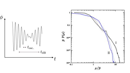
Figure 4: Left panel: a schematic illustration of the time dependence of the scalar $\phi$ at some fixed location. It has short time scale $t_{\rm osc.}=2\pi/m$ oscillations (around $\phi=0$), and long time scale $t_{\rm dB}=2\pi/(mv^{2})$ modulations. In practice, $t_{\rm dB}\gg t_{\rm osc.}$. Right panel: the one-point probability distribution of density in two wave dark matter halos. Here, $P(\rho)d\rho$ gives the probability that the density $\rho$ takes the values within the interval $d\rho$ and $\bar{\rho}$ is the (local) mean density. The solid lines are measured from numerical wave simulations of two halos that form from mergers of smaller seed halos and gravitational collapse. The blue line (II) is for a case where the halo is well-mixed, and the black line (I) is for a case where the halo retains some memory of the initial conditions. The blue dotted line shows the analytic prediction from the random phase halo model, $\bar{\rho}P(\rho)=e^{-\rho/\bar{\rho}}$, which describes case II well. The black dotted line is an approximate fit to case I: $\bar{\rho}P(\rho)=0.9\,e^{-1.06(\rho/\bar{\rho})^{2}}+0.1\,e^{-0.42(\rho/\bar{\rho})}$. Figure adapted from Hui et al. (2020).

The time variation of $\phi$ at a fixed location is depicted in the left panel of Figure 4. In addition, $\phi$ fluctuates spatially because $\psi$ does, on the de Broglie length scale $\lambda_{\rm dB}$ (Equation 1 and Figure 1). In other words, because the halo is composed of a superposition of waves of largely random phases, the wavefunction $\psi$ is essentially a stochastic field, which imprints $\sim t_{\rm dB}$ temporal modulations and $\sim\lambda_{\rm dB}$ spatial fluctuations on the axion $\phi$. Existing experiments are sensitive to a wide range of axion masses, from $m\sim 10^{-22}$ to $10^{-3}$ eV, though with significant gaps (Graham et al., 2015, Irastorza & Redondo, 2018, Sikivie, 2020). In many cases, time scales from $t_{\rm osc.}$ to $t_{\rm dB}$ and beyond are accessible to experiments.

A simple starting point for thinking about the stochastic fluctuations is the random phase halo model, spelled out in Equation 25: $\psi$ consists of a set of plane waves each with an amplitude $A_{\vec{k}}$ that depends on momentum $\vec{k}$, and a random phase. A simple distribution of momentum would be $A_{\vec{k}}\propto e^{-k^{2}/k_{0}^{2}}$, essentially an isothermal one, though other distributions are possible. In the random phase model, $\psi$ is a Gaussian random field obeying:

$$\langle\psi(t_{1},\vec{x}_{1})\psi^{*}(t_{2},\vec{x}_{2})\rangle=\sum_{\vec{k}}A_{\vec{k}}^{2}\,e^{i\vec{k}\cdot(\vec{x}_{1}-\vec{x}_{2})-i\omega_{k}(t_{1}-t_{2})}\quad,\quad\langle\psi(t_{1},\vec{x}_{1})\psi(t_{2},\vec{x}_{2})\rangle=0\,.$$ (45)

The higher point correlation functions obey Wick’s theorem, expressible as products of the two-point function. From this, all statistical properties of the axion $\phi$ follow, such as:

$$\langle\phi(t_{1},\vec{x}_{1})\phi(t_{2},\vec{x}_{2})\rangle={1\over 2m}\left(\langle\psi(t_{1},\vec{x}_{1})\psi^{*}(t_{2},\vec{x}_{2})\rangle e^{-im(t_{1}-t_{2})}+{\,\rm c.c.}\right)\,,$$ (46)

where ${\,\rm c.c.}$ represents complex conjugate. The Gaussian random nature of $\psi$ tells us the one-point probability distribution is Gaussian, specifically a two-dimensional one since $\psi$ has real and imaginary parts i.e. the Gaussian probability density ${\,\rm exp}[-|\psi|^{2}/(2\Gamma^{2})]$, where $\Gamma^{2}\equiv\sum_{\vec{k}}A_{\vec{k}}^{2}/2$, should come with the measure $d{\rm Re}\psi\,d{\rm Im}\psi=2\pi|\psi|d|\psi|$. In other words,

$$d|\psi|{|\psi|\over\Gamma^{2}}{\,\rm exp}\left[-{|\psi|^{2}\over 2\Gamma^{2}}\right]\,,$$ (47)

gives the probability that $|\psi|$ takes the values within the interval $d|\psi|$ (Centers et al., 2019). It can be checked that this is properly normalized. Recalling the density is $\rho=m|\psi|^{2}$, so average density is $\bar{\rho}=m\langle|\psi|^{2}\rangle=m^{2}\langle\phi^{2}\rangle=2m\Gamma^{2}$, the one-point distribution of density is thus:

$${d\rho\over\bar{\rho}}e^{-\rho/\bar{\rho}}\,.$$ (48)

There is a non-negligible probability for the density to fluctuate to low values, indeed all the way to zero (i.e. at sites of complete destructive interference or vortices). The right panel of Figure 4 shows a comparison of this analytic prediction with results from numerical simulations of two halos that form from mergers and gravitational collapse, taken from Hui et al. (2020). The analytic prediction works reasonably well, especially in the case (II) where the halo is well mixed. It works less well in the case (I) where some memory of the initial conditions persists—the halo has coherent substructures in the form of subhalos. See also Veltmaat et al. (2018) for correlation function measurements from numerical simulations.

The stochastic nature of the axion field $\phi$ and its derivatives has rich implications for axion detection. For instance, given the average local density $\bar{\rho}$ ($\sim 0.4{\,\rm GeV/cm^{3}}$), an axion experiment would sample from the whole distribution of $\rho$’s depicted in Figure 4, if time scales longer than the de Broglie time $t_{\rm dB}$ were accessible. In particular, there would be a non-negligible probability of sampling $\rho<\bar{\rho}$. As pointed out by Centers et al. (2019), experimental constraints on the axion couplings, such as $g_{\gamma}$ or $g_{\Psi}$, should take this into account. The full implications remain to be explored—depending on the experiment of interest, the relevant correlation function can be obtained by taking suitable derivatives of Equation 46.

Moreover, the stochastic nature of $\phi$ suggests it would be useful to measure correlation functions. For instance, the signal for ADMX (Du et al., 2018a) is often expressed in terms of the power output in a microwave cavity, which is proportional to $\phi^{2}$, or $\phi^{2}$ averaged over the rapid, frequency $m$ oscillations. One can consider the following correlation function in time (coincident location):

$$\langle\phi(t_{1})^{2}\phi(t_{2})^{2}\rangle-\langle\phi^{2}\rangle^{2}={1\over m^{2}}|\langle\psi(t_{1})\psi^{*}(t_{2})\rangle|^{2}={\bar{\rho}^{2}\over m^{4}}\left(1+{k_{0}^{4}(t_{1}-t_{2})^{2}\over 16m^{2}}\right)^{-3/2}\,,$$ (49)

where we have implicitly averaged $\phi^{2}(t)$ over the rapid oscillations, and assumed the random phase model. Here, $k_{0}$ is the rms (3D) momentum times $2/\sqrt{3}$, following from the distribution $A_{\vec{k}}^{2}\propto e^{-2k^{2}/k_{0}^{2}}$. This correlation function can be measured in a microwave cavity experiment. The characteristic power-law decay at large time separation might be helpful in pulling signal out of noisy data. Some experiments measure $\dot{\phi}$ by searching for a time varying magnetic flux produced by the oscillating axion in the presence of an external magnetic field, such as ABRACADABRA (Kahn et al., 2016, Ouellet et al., 2019). Others are sensitive to $\vec{\nabla}\phi$, such as CASPEr (Graham & Rajendran, 2013, Budker et al., 2014) or spin pendulum experiments (Terrano et al., 2019). The idea is to measure the spin precession around the direction picked out by $\vec{\nabla}\phi$, using the axion-fermion coupling (Equation 9). Correlation functions thereof can be obtained by differentiating Equation 46.

More generally, with a network of detectors, one can measure the correlation function in space-time:

$$\langle\phi(t_{1},\vec{x}_{1})^{2}\phi(t_{2},\vec{x}_{2})^{2}\rangle-\langle\phi^{2}\rangle^{2}={\bar{\rho}{}^{2}\over m^{4}}\left(1+\frac{k_{0}^{4}(t_{1}-t_{2})^{2}}{16m^{2}}\right)^{-3/2}\exp\left(-\frac{4k_{0}^{2}m^{2}\lvert\vec{x}_{1}-\vec{x}_{2}\rvert^{2}}{16m^{2}+k_{0}^{4}(t_{1}-t_{2})^{2}}\right)\,,$$ (50)

where again we have implicitly averaged over the rapid oscillations. The difference in dependence on time-separation versus space-separation originates from the fact $\omega_{k}$, the frequency for a Fourier mode, goes as $k^{2}$ rather than $k$. The idea of using a network of detectors, much like an interferometry array in radio astronomy, has been discussed in Pustelny et al. (2013) for GNOME, and in Derevianko (2018), Foster et al. (2018), Roberts et al. (2017), Savalle et al. (2019), Centers et al. (2019), Hui et al. (2020), Foster et al. (2020b). Experiments that measure the rotation of photon polarization in an axion background naturally measures $\phi$ at points separated in time and/or space (Liu et al., 2019, DeRocco & Hook, 2018, Martynov & Miao, 2020).

It is worth pointing out that different experiments respond differently to the passing of a vortex. As discussed in Section 4.4, at the location of a vortex, $\psi$ vanishes but its gradient generically does not. This implies experiments that probe $\phi$ or $\dot{\phi}$ have a vanishing signal while those that probe $\vec{\nabla}\phi$ have a non-vanishing one. Perhaps more interesting is how the generic existence of vortices (one vortex ring per de Broglie volume) points to interesting structures in the phase of the axion oscillations. Plugging $\psi=\sqrt{\rho/m}\,e^{i\theta}$ into Equation 43, the axion field $\phi$ can be expressed as:

$$\phi(t,\vec{x})=m^{-1}\sqrt{2\rho(t,\vec{x})}{\,\rm cos\,}\left[mt-\theta(t,\vec{x})\right]\,.$$ (51)

Dark matter detection, for good reasons, generally focuses on measuring the amplitude of the axion oscillations, which tells us about the density of dark matter $\rho$. The arguments in Section 4.4 tell us wave interference generically produces non-trivial structures in the oscillation phase $\theta(t,\vec{x})$ i.e. winding around vortices. It would be useful to explore how such winding could be measured, how it might be exploited to enhance detection sensitivity. Doing so likely requires a network of detectors, possibly combining different detection techniques that get at different derivatives of $\phi$ (Hui et al., 2020).

6 Discussion—theory exploration, numerical simulations, astrophysical probes and experimental detection

We have reviewed the particle physics motivations for considering wave dark matter, and the observational and experimental implications, with the axion as the prime example. We close with a list of open questions and directions for further research.

Theory exploration. The dark matter sector could well be as rich as the visible sector, with different kinds of particles. This has a certain plausibility in string theory, which generically predicts a variety of axions. Most of them would be too massive to be a suitable dark matter candidate. But if one of them is light enough to be dark matter, perhaps there maybe more (Arvanitaki et al., 2010, Bachlechner et al., 2019, Luu et al., 2020)? And if these light axions are coupled, how is the relic abundance computation modified? What is the impact on galactic substructures if there is a mixture of wave and particle dark matter, or a mixture of wave dark matter of different masses (Schwabe et al., 2020)? If the axion as a field exists during inflation, it has inevitable isocurvature fluctuations—if the energy scale of inflation is high enough to saturate the existing isocurvature bound, what are the implications for structure formation (Section 5.1)?

Numerical simulations. There is a great need for more and better simulations of wave dark matter structure formation. Some of the existing constraints at the ultra-light end of the spectrum ($10^{-22}-10^{-20}$ eV, fuzzy dark matter) rely on the halo or subhalo mass function that has not been checked with wave simulations (Section 5.3). Current estimates of the halo/subhalo mass function account for the wave nature of dark matter primarily through its impact on the initial condition i.e. the primordial power spectrum (Section 5.2). It is important to quantify how the wave dynamics affects the subsequent evolution. Further simulations would also be useful for interpreting constraints from galaxy density profiles (by including the effects of baryons and tidal forces), and constraints from the Lyman-alpha forest (by exploring the variety of fluctuations from the ionizing background, reionization history and galactic winds). There is also room for improvement in numerical algorithm: it is challenging to carry out wave simulations in large boxes with the requisite de-Broglie-scale resolution (Section 4.3). The hybrid scheme of Veltmaat et al. (2018) is one promising approach. In addition, there is a need for more simulations of the early universe. If the Peccei-Quinn symmetry is broken after inflation, large fluctuations are expected to lead to axion star formation (Kolb & Tkachev, 1993). An accurate mass function of such objects, accounting for the effect of subsequent mergers (Eggemeier & Niemeyer, 2019), would be very useful. The axion in question can span a large range in mass and need not be ultra-light (Sections 4.2 and 5.4).

Astrophysical probes. A striking prediction of wave dark matter is the interference substructures inside a halo. These are order unity density fluctuations on the scale of the de Broglie wavelength. The density can even vanish, where complete destructive interference occurs. These are locations of vortices—a unique wave phenomenon (Section 4.4). Such interference patterns are distinct from subhalos as a form of halo substructure. Some observational signatures, for ultra-light masses, have been worked out, such as the scattering of stars and gravitational lensing (Section 5.3). Recent measurements of the density power spectrum along globular cluster tidal streams GD-1 and Palomar 5, from Gaia and Pan-STARRS data, suggest consistency with scattering by subhalos in conventional cold dark matter (Bovy et al., 2017, Banik et al., 2019a, b). Are the same measurements consistent with fuzzy dark mater? To answer this question, one must account for scattering by both the subhalo contents (Schutz, 2020) and the interference substructures (Dalal et al., 2020). In addition, it is important to clarify to what extent the tidal stream density fluctuations can be attributed to the tidal disruption process itself (Kuepper et al., 2010, Ibata et al., 2020). More measurements spanning different orbital radii would be helpful in differentiating between models: scattering by interference substructures is expected to be more important at small radii relative to scattering by subhalos (Dalal et al., 2020). It is also worth noting there are other statistics that might have different sensitivity to the mass and compactness of subhalos (e.g. Bonaca et al., 2018). Improvement in stellar stream data is expected from further Gaia data release and the upcoming Vera Rubin Observatory (Ivezić et al., 2019).

Anomalous flux ratios between gravitationally lensed images have been used to constrain substructures in galaxy lenses (Hezaveh et al., 2016b, Hsueh et al., 2020, Gilman et al., 2019, Dai et al., 2020). See Section 5.3. Typically these constraints are obtained by fitting the data with a parametrized model of subhalos, which is then checked against the prediction of conventional cold dark matter. For fuzzy dark matter, two issues should be addressed. One is a proper wave computation of the subhalo mass function, discussed earlier. The other is the inclusion of wave interference substructures as an additional source of flux anomaly (Chan et al., 2020, Hui et al., 2020). This is a promising technique given the expected improvement in lensing data, e.g. from ALMA (Vlahakis et al., 2015, Hezaveh et al., 2016b).

Observations of the high redshift ($z>5$) universe have the potential to probe the linear power spectrum on small scales, and therefore constrain fuzzy dark matter, as discussed in Section 5.2. Promising future data include those from the James Webb Space Telescope (Gardner et al., 2006, Hirano et al., 2018) and 21cm experiments (DeBoer et al., 2017, Weltman et al., 2020, Bowman et al., 2018). To take full advantage of these data, the fuzzy dark matter predictions for early structure formation should be refined using wave simulations in larger boxes (Mocz et al., 2019, May & Springel, 2021).

Another area where more data are needed is the study of dynamical friction. The Fornax dwarf galaxy is the main example where there is possibly a dynamical friction problem—that its globular clusters survive in its halo despite efficient dynamical friction (Tremaine, 1976, Oh et al., 2000). One resolution is to invoke fuzzy dark matter to weaken dynamical friction, though it appears core stalling might also do the job (see Sections 4.5 and 5.3). Data on more such systems would be instructive.

Detection experiments. The interference substructures are a robust prediction of wave dark matter, regardless of the dark matter mass. Away from the ultra-light end of the spectrum, the corresponding de Broglie wavelength is small, making the interference substructures challenging to observe astrophysically. But the substructures remain relevant for axion detection experiments which are sensitive to much smaller scales. The axion field is effectively stochastic, in a halo made out of a superposition of waves with random phases. At a minimum, this stochastic nature should be accounted for in deriving constraints. Moreover, the stochastic nature motivates the measurement of correlation functions of the axion field. The correlation can involve both time and space separations, further motivating the idea of a network of detectors, like in radio interferometry. An under-explored area is the information contained in the phase of the axion oscillations (Equation 51). That vortices generically exist tells us there are non-trivial structures in the phase, such as winding. An interesting question is whether searching for such structures might help extract signal out of noisy data (Section 5.6).

DISCLOSURE STATEMENT

The author is not aware of any affiliations, memberships, funding, or financial holdings that might be perceived as affecting the objectivity of this review.

References

- Abbott & Sikivie (1983) Abbott L, Sikivie P. 1983. Phys. Lett. B 120:133–136
- Aghanim et al. (2020) Aghanim N, et al. 2020. Astron. Astrophys. 641:A6
- Agrawal et al. (2020) Agrawal P, Hook A, Huang J. 2020. JHEP 07:138
- Akiyama et al. (2019) Akiyama K, et al. 2019. Astrophys. J. Lett. 875:L5
- Alexander et al. (2019) Alexander S, Bramburger JJ, McDonough E. 2019. Phys. Lett. B 797:134871
- Alexander & Cormack (2017) Alexander S, Cormack S. 2017. JCAP 1704:005
- Alexander et al. (2020) Alexander S, Gleyzer S, McDonough E, Toomey MW, Usai E. 2020. Astrophys. J. 893:15
- Allali & Hertzberg (2020) Allali I, Hertzberg MP. 2020. JCAP 07:056
- Alonso-Álvarez & Jaeckel (2018) Alonso-Álvarez G, Jaeckel J. 2018. JCAP 10:022
- Amendola & Barbieri (2006) Amendola L, Barbieri R. 2006. Phys. Lett. B642:192–196
- Amin et al. (2012) Amin MA, Easther R, Finkel H, Flauger R, Hertzberg MP. 2012. Phys. Rev. Lett. 108:241302
- Amorisco & Evans (2012) Amorisco N, Evans N. 2012. Mon. Not. Roy. Astron. Soc. 419:184–196
- Amorisco & Loeb (2018) Amorisco NC, Loeb A. 2018. arXiv:1808.00464
- Anastassopoulos et al. (2017) Anastassopoulos V, et al. 2017. Nature Phys. 13:584–590
- Annulli et al. (2020) Annulli L, Cardoso V, Vicente R. 2020. Phys. Rev. D 102:063022
- Aoki & Mukohyama (2016) Aoki K, Mukohyama S. 2016. Phys. Rev. D 94:024001
- Armengaud et al. (2017) Armengaud E, Palanque-Delabrouille N, Yèche C, Marsh DJ, Baur J. 2017. Mon. Not. Roy. Astron. Soc. 471:4606–4614
- Arvanitaki et al. (2017) Arvanitaki A, Baryakhtar M, Dimopoulos S, Dubovsky S, Lasenby R. 2017. Phys. Rev. D 95:043001
- Arvanitaki et al. (2010) Arvanitaki A, Dimopoulos S, Dubovsky S, Kaloper N, March-Russell J. 2010. Phys. Rev. D81:123530
- Arvanitaki et al. (2020) Arvanitaki A, Dimopoulos S, Galanis M, Lehner L, Thompson JO, Van Tilburg K. 2020. Phys. Rev. D 101:083014
- Arvanitaki & Dubovsky (2011) Arvanitaki A, Dubovsky S. 2011. Phys. Rev. D83:044026
- Axenides et al. (1983) Axenides M, Brandenberger RH, Turner MS. 1983. Phys. Lett. B 126:178–182
- Bachlechner et al. (2019) Bachlechner TC, Eckerle K, Janssen O, Kleban M. 2019. JCAP 1909:062
- Bai & Hamada (2018) Bai Y, Hamada Y. 2018. Phys. Lett. B 781:187–194
- Baldeschi et al. (1983) Baldeschi MR, Ruffini R, Gelmini GB. 1983. Phys. Lett. 122B:221–224
- Bamber et al. (2020) Bamber J, Clough K, Ferreira PG, Hui L, Lagos M. 2020. arXiv:2011.07870
- Banik et al. (2019a) Banik N, Bovy J, Bertone G, Erkal D, de Boer T. 2019a. arXiv:1911.02662
- Banik et al. (2019b) Banik N, Bovy J, Bertone G, Erkal D, de Boer T. 2019b. arXiv:1911.02663
- Banik & Sikivie (2013) Banik N, Sikivie P. 2013. Phys. Rev. D88:123517
- Bar et al. (2018) Bar N, Blas D, Blum K, Sibiryakov S. 2018. Phys. Rev. D98:083027
- Bar et al. (2020) Bar N, Blum K, D’Amico G. 2020. Phys. Rev. D 101:123025
- Bar et al. (2019a) Bar N, Blum K, Eby J, Sato R. 2019a. Phys. Rev. D 99:103020
- Bar et al. (2019b) Bar N, Blum K, Lacroix T, Panci P. 2019b. JCAP 07:045
- Bar-Or et al. (2019) Bar-Or B, Fouvry JB, Tremaine S. 2019. Astrophys. J. 871:28
- Barausse et al. (2014) Barausse E, Cardoso V, Pani P. 2014. Phys. Rev. D 89:104059
- Bardeen et al. (1972) Bardeen JM, Press WH, Teukolsky SA. 1972. Astrophys. J. 178:347
- Barkana et al. (2001) Barkana R, Haiman Z, Ostriker JP. 2001. Astrophys. J. 558:482
- Barranco et al. (2012) Barranco J, Bernal A, Degollado JC, Diez-Tejedor A, Megevand M, et al. 2012. Phys. Rev. Lett. 109:081102
- Baumann (2011) Baumann D. 2011. Inflation. In Theoretical Advanced Study Institute in Elementary Particle Physics: Physics of the Large and the Small
- Baumann et al. (2019) Baumann D, Chia HS, Porto RA. 2019. Phys. Rev. D 99:044001
- Bekenstein (1972a) Bekenstein J. 1972a. Phys. Rev. D 5:2403–2412
- Bekenstein (1972b) Bekenstein JD. 1972b. Phys. Rev. D 5:1239–1246
- Bennett et al. (2013) Bennett CL, Larson D, Weiland JL, Jarosik N, Hinshaw G, et al. 2013. ApJS 208:20
- Berezhiani et al. (2019) Berezhiani L, Elder B, Khoury J. 2019. JCAP 10:074
- Berezhiani & Khoury (2015a) Berezhiani L, Khoury J. 2015a. Phys. Rev. D92:103510
- Berezhiani & Khoury (2015b) Berezhiani L, Khoury J. 2015b. Phys. Rev. D92:103510
- Bezerra et al. (2014) Bezerra VB, Vieira HS, Costa AA. 2014. Class. Quant. Grav. 31:045003
- Bialynicki-Birula et al. (2000) Bialynicki-Birula I, Bialynicka-Birula Z, Śliwa C. 2000. Phys. Rev. A 61:032110
- Binney & Tremaine (2008) Binney J, Tremaine S. 2008. Galactic Dynamics, 2nd ed. Princeton, NJ, Princeton University Press
- Bird et al. (2016) Bird S, Cholis I, Muñoz JB, Ali-Haïmoud Y, Kamionkowski M, et al. 2016. Phys. Rev. Lett. 116:201301
- Blas et al. (2020) Blas D, Caputo A, Ivanov MM, Sberna L. 2020. Phys. Dark Univ. 27:100428
- Bonaca et al. (2018) Bonaca A, Hogg DW, Price-Whelan AM, Conroy C. 2018. arXiv:1811.03631
- Bovy et al. (2017) Bovy J, Erkal D, Sanders JL. 2017. Mon. Not. Roy. Astron. Soc. 466:628–668
- Bovy & Tremaine (2012) Bovy J, Tremaine S. 2012. Astrophys. J. 756:89
- Bowman et al. (2018) Bowman JD, Rogers AEE, Monsalve RA, Mozdzen TJ, Mahesh N. 2018. Nature 555:67–70
- Brax et al. (2020) Brax P, Cembranos JA, Valageas P. 2020. Phys. Rev. D 101:023521
- Brook & Coles (2009) Brook MN, Coles P. 2009. arXiv:0902.0605
- Budker et al. (2014) Budker D, Graham PW, Ledbetter M, Rajendran S, Sushkov A. 2014. Phys. Rev. X4:021030
- Burkert (2020) Burkert A. 2020. arXiv:2006.11111
- Buschmann et al. (2020) Buschmann M, Foster JW, Safdi BR. 2020. Phys. Rev. Lett. 124:161103
- Calabrese & Spergel (2016) Calabrese E, Spergel DN. 2016. Mon. Not. Roy. Astron. Soc. 460:4397–4402
- Caputo et al. (2019) Caputo A, Sberna L, Frias M, Blas D, Pani P, et al. 2019. Phys. Rev. D 100:063515
- Carroll & Field (1997) Carroll SM, Field GB. 1997. Phys. Rev. Lett. 79:2394–2397
- Carroll et al. (1990) Carroll SM, Field GB, Jackiw R. 1990. Phys. Rev. D 41:1231
- Cen et al. (2009) Cen R, McDonald P, Trac H, Loeb A. 2009. Astrophys. J. 706:L164–L167
- Centers et al. (2019) Centers GP, et al. 2019. arXiv:1905.13650
- Chambers et al. (2019) Chambers KC, Magnier EA, Metcalfe N, Flewelling HA, Huber ME, et al. 2019. arXiv:1612.05560
- Chan et al. (2020) Chan JH, Schive HY, Wong SK, Chiueh T, Broadhurst T. 2020. Phys. Rev. Lett. 125:111102
- Chavanis (2011) Chavanis PH. 2011. Phys. Rev. D84:043531
- Chavanis (2019) Chavanis PH. 2019. Eur. Phys. J. Plus 134:352
- Chen et al. (2017) Chen SR, Schive HY, Chiueh T. 2017. Mon. Not. Roy. Astron. Soc. 468:1338–1348
- Chiba (2002) Chiba M. 2002. Astrophys. J. 565:17
- Chiueh et al. (2011) Chiueh T, Woo TP, Jian HY, Schive HY. 2011. Journal of Physics B 44:115101
- Chluba et al. (2019) Chluba J, et al. 2019. arXiv:1909.01593
- Choi & Im (2016) Choi K, Im SH. 2016. JHEP 01:149
- Church et al. (2019) Church BV, Ostriker JP, Mocz P. 2019. Mon. Not. Roy. Astron. Soc. 485:2861–2876
- Clough et al. (2018) Clough K, Dietrich T, Niemeyer JC. 2018. Phys. Rev. D 98:083020
- Clough et al. (2019) Clough K, Ferreira PG, Lagos M. 2019. Phys. Rev. D100:063014
- Clowe et al. (2006) Clowe D, Bradač M, Gonzalez AH, Markevitch M, Randall SW, et al. 2006. ApJ 648:L109–L113
- Co et al. (2020) Co RT, Hall LJ, Harigaya K. 2020. Phys. Rev. Lett. 124:251802
- Cole et al. (2012) Cole DR, Dehnen W, Read JI, Wilkinson MI. 2012. Mon. Not. Roy. Astron. Soc. 426:601
- Cookmeyer et al. (2020) Cookmeyer J, Grin D, Smith TL. 2020. Phys. Rev. D 101:023501
- Croft et al. (1998) Croft R, Weinberg DH, Katz N, Hernquist L. 1998. Astrophys. J. 495:44–62
- Croft (2004) Croft RA. 2004. Astrophys. J. 610:642–662
- Dai et al. (2020) Dai L, Kaurov AA, Sharon K, Florian MK, Miralda-Escudé J, et al. 2020. Mon. Not. Roy. Astron. Soc. 495:3192–3208
- Dalal et al. (2020) Dalal N, Bovy J, Hui L, Li X. 2020. arXiv:2011.13141
- Dalal & Kochanek (2002) Dalal N, Kochanek CS. 2002. Astrophys. J. 572:25–33
- D’Aloisio et al. (2018) D’Aloisio A, McQuinn M, Davies FB, Furlanetto SR. 2018. Mon. Not. Roy. Astron. Soc. 473:560–575
- Damour et al. (1976) Damour T, Deruelle N, Ruffini R. 1976. Lett. Nuovo Cim. 15:257–262
- Davies & Mocz (2020) Davies EY, Mocz P. 2020. Mon. Not. Roy. Astron. Soc. 492:5721–5729
- Davoudiasl & Denton (2019) Davoudiasl H, Denton PB. 2019. Phys. Rev. Lett. 123:021102
- Davoudiasl & Murphy (2017) Davoudiasl H, Murphy CW. 2017. Phys. Rev. Lett. 118:141801
- De Martino et al. (2020) De Martino I, Broadhurst T, Tye SHH, Chiueh T, Schive HY. 2020. Phys. Dark Univ. 28:100503
- DeBoer et al. (2017) DeBoer DR, et al. 2017. Publ. Astron. Soc. Pac. 129:045001
- Derevianko (2018) Derevianko A. 2018. Phys. Rev. A97:042506
- DeRocco et al. (2020) DeRocco W, Graham PW, Rajendran S. 2020. Phys. Rev. D 102:075015
- DeRocco & Hook (2018) DeRocco W, Hook A. 2018. Phys. Rev. D 98:035021
- Desjacques et al. (2018) Desjacques V, Kehagias A, Riotto A. 2018. Phys. Rev. D 97:023529
- Detweiler (1980) Detweiler SL. 1980. Phys. Rev. D22:2323–2326
- Dietrich & Clough (2019) Dietrich T, Clough K. 2019. Phys. Rev. D 100:083005
- Dine (2000) Dine M. 2000. TASI lectures on the strong CP problem. In Theoretical Advanced Study Institute in Elementary Particle Physics (TASI 2000): Flavor Physics for the Millennium
- Dine (2016) Dine M. 2016. Supersymmetry and String Theory: Beyond the Standard Model. Cambridge University Press
- Dine & Fischler (1983) Dine M, Fischler W. 1983. Phys. Lett. B 120:137–141
- Dine et al. (1981) Dine M, Fischler W, Srednicki M. 1981. Phys. Lett. B 104:199–202
- Dolan (2007) Dolan SR. 2007. Phys. Rev. D76:084001
- Du et al. (2018a) Du N, et al. 2018a. Phys. Rev. Lett. 120:151301
- Du et al. (2017) Du X, Behrens C, Niemeyer JC. 2017. Mon. Not. Roy. Astron. Soc. 465:941–951
- Du et al. (2018b) Du X, Schwabe B, Niemeyer JC, Bürger D. 2018b. Phys. Rev. D 97:063507
- Dvali & Zell (2018) Dvali G, Zell S. 2018. JCAP 07:064
- Easther et al. (2009) Easther R, Giblin John T. J, Hui L, Lim EA. 2009. Phys. Rev. D 80:123519
- Eby et al. (2016a) Eby J, Kouvaris C, Nielsen NG, Wijewardhana L. 2016a. JHEP 02:028
- Eby et al. (2016b) Eby J, Suranyi P, Wijewardhana L. 2016b. Mod. Phys. Lett. A 31:1650090
- Edwards et al. (2018) Edwards F, Kendall E, Hotchkiss S, Easther R. 2018. JCAP 1810:027
- Eggemeier & Niemeyer (2019) Eggemeier B, Niemeyer JC. 2019. Phys. Rev. D 100:063528
- Ellis & Olive (1987) Ellis JR, Olive KA. 1987. Phys. Lett. B 193:525
- Endlich & Penco (2017) Endlich S, Penco R. 2017. JHEP 05:052
- Fairbairn et al. (2018) Fairbairn M, Marsh DJE, Quevillon J, Rozier S. 2018. Phys. Rev. D 97:083502
- Fan (2016) Fan J. 2016. Phys. Dark Univ. 14:84–94
- Fedderke et al. (2019) Fedderke MA, Graham PW, Rajendran S. 2019. Phys. Rev. D 100:015040
- Felder & Tkachev (2008) Felder GN, Tkachev I. 2008. Comput. Phys. Commun. 178:929–932
- Fetter (2008) Fetter AL. 2008. Laser Physics 18:1–11
- Feynman et al. (1963) Feynman RP, Leighton RB, Sands M. 1963. The Feynman Lectures on Physics. Addison Wesley Longman
- Ficarra et al. (2019) Ficarra G, Pani P, Witek H. 2019. Phys. Rev. D 99:104019
- Foster et al. (2020a) Foster JW, Kahn Y, Macias O, Sun Z, Eatough RP, et al. 2020a. Phys. Rev. Lett. 125:171301
- Foster et al. (2020b) Foster JW, Kahn Y, Nguyen R, Rodd NL, Safdi BR. 2020b. arXiv:2009.14201
- Foster et al. (2018) Foster JW, Rodd NL, Safdi BR. 2018. Phys. Rev. D97:123006
- Freeman (1970) Freeman K. 1970. Astrophys. J. 160:811
- Friedberg et al. (1987a) Friedberg R, Lee T, Pang Y. 1987a. Phys. Rev. D 35:3640
- Friedberg et al. (1987b) Friedberg R, Lee T, Pang Y. 1987b. Phys. Rev. D 35:3658
- Garcia-Bellido & Ruiz Morales (2017) Garcia-Bellido J, Ruiz Morales E. 2017. Phys. Dark Univ. 18:47–54
- Gardner et al. (2006) Gardner JP, et al. 2006. Space Sci. Rev. 123:485
- Garny et al. (2020) Garny M, Konstandin T, Rubira H. 2020. JCAP 04:003
- Giblin et al. (2010) Giblin John T. J, Hui L, Lim EA, Yang IS. 2010. Phys. Rev. D 82:045019
- Gilman et al. (2020) Gilman D, Birrer S, Nierenberg A, Treu T, Du X, Benson A. 2020. Mon. Not. Roy. Astron. Soc. 491:6077–6101
- Gilman et al. (2019) Gilman D, Birrer S, Treu T, Nierenberg A, Benson A. 2019. Mon. Not. Roy. Astron. Soc. 487:5721–5738
- Glauber (1963) Glauber RJ. 1963. Phys. Rev. 130:2529–2539
- Goerdt et al. (2006) Goerdt T, Moore B, Read J, Stadel J, Zemp M. 2006. Mon. Not. Roy. Astron. Soc. 368:1073–1077
- Gondolo & Silk (2000) Gondolo P, Silk J. 2000. Nucl. Phys. B Proc. Suppl. 87:87–89
- Goodman (2000) Goodman J. 2000. New Astron. 5:103
- Gorghetto et al. (2020) Gorghetto M, Hardy E, Villadoro G. 2020. arXiv:2007.04990
- Graham et al. (2015) Graham PW, Irastorza IG, Lamoreaux SK, Lindner A, van Bibber KA. 2015. Ann. Rev. Nucl. Part. Sci. 65:485–514
- Graham et al. (2016a) Graham PW, Kaplan DE, Mardon J, Rajendran S, Terrano WA. 2016a. Phys. Rev. D 93:075029
- Graham et al. (2016b) Graham PW, Mardon J, Rajendran S. 2016b. Phys. Rev. D 93:103520
- Graham & Rajendran (2013) Graham PW, Rajendran S. 2013. Phys. Rev. D88:035023
- Green et al. (1988) Green MB, Schwarz J, Witten E. 1988. SUPERSTRING THEORY. VOL. 2: LOOP AMPLITUDES, ANOMALIES AND PHENOMENOLOGY
- Grilli di Cortona et al. (2016) Grilli di Cortona G, Hardy E, Pardo Vega J, Villadoro G. 2016. JHEP 01:034
- Grillmair & Dionatos (2006) Grillmair CJ, Dionatos O. 2006. Astrophys. J. Lett. 643:L17–L20
- Guth et al. (2015) Guth AH, Hertzberg MP, Prescod-Weinstein C. 2015. Phys. Rev. D92:103513
- Guzman & Urena-Lopez (2006a) Guzman F, Urena-Lopez L. 2006a. Astrophys. J. 645:814–819
- Guzman & Urena-Lopez (2006b) Guzman FS, Urena-Lopez LA. 2006b. Astrophys. J. 645:814–819
- Halverson et al. (2017) Halverson J, Long C, Nath P. 2017. Phys. Rev. D96:056025
- Hannuksela et al. (2019) Hannuksela OA, Wong KW, Brito R, Berti E, Li TG. 2019. Nature Astron. 3:447–451
- Harari & Sikivie (1992) Harari D, Sikivie P. 1992. Phys. Lett. B 289:67–72
- Harrison et al. (2003) Harrison R, Moroz I, Tod KP. 2003. Nonlinearity 16:101–122
- Helfer et al. (2019) Helfer T, Lim EA, Garcia MA, Amin MA. 2019. Phys. Rev. D 99:044046
- Helfer et al. (2017) Helfer T, Marsh DJE, Clough K, Fairbairn M, Lim EA, Becerril R. 2017. JCAP 03:055
- Hertzberg & Schiappacasse (2018) Hertzberg MP, Schiappacasse ED. 2018. JCAP 1808:028
- Hezaveh et al. (2016a) Hezaveh Y, Dalal N, Holder G, Kisner T, Kuhlen M, Perreault Levasseur L. 2016a. JCAP 1611:048
- Hezaveh et al. (2016b) Hezaveh YD, et al. 2016b. Astrophys. J. 823:37
- Higaki et al. (2014) Higaki T, Jeong KS, Takahashi F. 2014. Phys. Lett. B 734:21–26
- Hills et al. (2018) Hills R, Kulkarni G, Meerburg PD, Puchwein E. 2018. Nature 564:E32–E34
- Hinshaw et al. (2013) Hinshaw G, et al. 2013. Astrophys. J. Suppl. 208:19
- Hirano et al. (2018) Hirano S, Sullivan JM, Bromm V. 2018. Mon. Not. Roy. Astron. Soc. 473:L6–L10
- Hložek et al. (2017) Hložek R, Marsh DJE, Grin D, Allison R, Dunkley J, Calabrese E. 2017. Phys. Rev. D 95:123511
- Hlozek et al. (2015) Hlozek R, Grin D, Marsh DJE, Ferreira PG. 2015. Phys. Rev. D91:103512
- Hoekstra et al. (2004) Hoekstra H, Yee HK, Gladders MD. 2004. Astrophys. J. 606:67–77
- Hook (2019) Hook A. 2019. PoS TASI2018:004
- Hook et al. (2018) Hook A, Kahn Y, Safdi BR, Sun Z. 2018. Phys. Rev. Lett. 121:241102
- Horbatsch & Burgess (2012) Horbatsch M, Burgess C. 2012. JCAP 05:010
- Hsueh et al. (2020) Hsueh JW, Enzi W, Vegetti S, Auger M, Fassnacht CD, et al. 2020. Mon. Not. Roy. Astron. Soc. 492:3047–3059
- Hu et al. (2000) Hu W, Barkana R, Gruzinov A. 2000. Phys. Rev. Lett. 85:1158–1161
- Hui (1999) Hui L. 1999. Astrophys. J. 516:519–526
- Hui & Gnedin (1997) Hui L, Gnedin NY. 1997. Mon. Not. Roy. Astron. Soc. 292:27
- Hui et al. (2020) Hui L, Joyce A, Landry MJ, Li X. 2020
- Hui et al. (2019) Hui L, Kabat D, Li X, Santoni L, Wong SSC. 2019. JCAP 1906:038
- Hui et al. (2017) Hui L, Ostriker JP, Tremaine S, Witten E. 2017. Phys. Rev. D95:043541
- Ibata et al. (2002) Ibata R, Lewis G, Irwin M. 2002. Mon. Not. Roy. Astron. Soc. 332:915
- Ibata et al. (2020) Ibata R, Thomas G, Famaey B, Malhan K, Martin N, Monari G. 2020. The Astrophysical Journal 891:161
- Ibata et al. (2016) Ibata RA, Lewis GF, Martin NF. 2016. The Astrophysical Journal 819:1
- Inoue (2011) Inoue S. 2011. Mon. Not. Roy. Astron. Soc. 416:1181–1190
- Irastorza & Redondo (2018) Irastorza IG, Redondo J. 2018. Prog. Part. Nucl. Phys. 102:89–159
- Iršič et al. (2017) Iršič V, Viel M, Haehnelt MG, Bolton JS, Becker GD. 2017. Phys. Rev. Lett. 119:031302
- Iršič et al. (2020) Iršič V, Xiao H, McQuinn M. 2020. Phys. Rev. D 101:123518
- Ivanov et al. (2019) Ivanov M, Kovalev Y, Lister M, Panin A, Pushkarev A, et al. 2019. JCAP 02:059
- Ivezić et al. (2019) Ivezić v, et al. 2019. Astrophys. J. 873:111
- Jacobson (1999) Jacobson T. 1999. Phys. Rev. Lett. 83:2699–2702
- Jedamzik (2020) Jedamzik K. 2020. JCAP 09:022
- Johnston et al. (2002) Johnston KV, Spergel DN, Haydn C. 2002. Astrophys. J. 570:656
- Kahn et al. (2016) Kahn Y, Safdi BR, Thaler J. 2016. Phys. Rev. Lett. 117:141801
- Kain & Ling (2010) Kain B, Ling HY. 2010. Phys. Rev. D82:064042
- Kaplan & Rattazzi (2016) Kaplan DE, Rattazzi R. 2016. Phys. Rev. D 93:085007
- Kaplinghat et al. (2020) Kaplinghat M, Ren T, Yu HB. 2020. JCAP 06:027
- Kato & Soda (2020) Kato R, Soda J. 2020. JCAP 09:036
- Kaup (1968) Kaup DJ. 1968. Phys. Rev. 172:1331–1342
- Keating et al. (2018) Keating LC, Puchwein E, Haehnelt MG. 2018. Mon. Not. Roy. Astron. Soc. 477:5501–5516
- Khmelnitsky & Rubakov (2014) Khmelnitsky A, Rubakov V. 2014. JCAP 1402:019
- Kim (1979) Kim JE. 1979. Phys. Rev. Lett. 43:103
- Kim & Marsh (2016) Kim JE, Marsh D. 2016. Phys. Rev. D93:025027
- Kobayashi et al. (2017) Kobayashi T, Murgia R, De Simone A, Iršič V, Viel M. 2017. Phys. Rev. D 96:123514
- Kogut et al. (2019) Kogut A, Abitbol M, Chluba J, Delabrouille J, Fixsen D, et al. 2019. arXiv:1907.13195
- Kolb & Long (2020) Kolb EW, Long AJ. 2020. arXiv:2009.03828
- Kolb & Tkachev (1993) Kolb EW, Tkachev II. 1993. Phys. Rev. Lett. 71:3051–3054
- Kolb & Tkachev (1996) Kolb EW, Tkachev II. 1996. Astrophys. J. Lett. 460:L25–L28
- Kolb & Turner (1990) Kolb EW, Turner MS. 1990. The Early Universe. vol. 69
- Konoplya & Zhidenko (2006) Konoplya RA, Zhidenko A. 2006. Phys. Rev. D73:124040
- Kuepper et al. (2010) Kuepper A, Kroupa P, Baumgardt H, Heggie D. 2010. Mon. Not. Roy. Astron. Soc. 401:105
- Kulkarni & Ostriker (2020) Kulkarni M, Ostriker JP. 2020. arXiv:2011.02116
- Lancaster et al. (2020) Lancaster L, Giovanetti C, Mocz P, Kahn Y, Lisanti M, Spergel DN. 2020. JCAP 01:001
- Lentz et al. (2020) Lentz EW, Quinn TR, Rosenberg LJ. 2020. Nucl. Phys. B 952:114937
- Lesgourgues et al. (2002) Lesgourgues J, Arbey A, Salati P. 2002. New Astron. Rev. 46:791–799
- Levkov et al. (2018) Levkov D, Panin A, Tkachev I. 2018. Phys. Rev. Lett. 121:151301
- Li et al. (2019) Li X, Hui L, Bryan GL. 2019. Phys. Rev. D99:063509
- Li et al. (2021) Li X, Hui L, Yavetz TD. 2021. Phys. Rev. D 103:023508
- Li et al. (2020) Li Z, Shen J, Schive HY. 2020. arXiv:2001.00318
- Lidz & Hui (2018) Lidz A, Hui L. 2018. Phys. Rev. D 98:023011
- Lin et al. (2018) Lin SC, Schive HY, Wong SK, Chiueh T. 2018. Phys. Rev. D 97:103523
- Linde (1985) Linde AD. 1985. Phys. Lett. B 158:375–380
- Liu & Ng (2017) Liu GC, Ng KW. 2017. Phys. Dark Univ. 16:22–25
- Liu et al. (2019) Liu H, Elwood BD, Evans M, Thaler J. 2019. Phys. Rev. D100:023548
- Lora et al. (2012) Lora V, Magana J, Bernal A, Sanchez-Salcedo FJ, Grebel EK. 2012. JCAP 1202:011
- Lue et al. (1999) Lue A, Wang LM, Kamionkowski M. 1999. Phys. Rev. Lett. 83:1506–1509
- Lund (1991) Lund F. 1991. Physics Letters A 159:245 – 251
- Luscher (1981) Luscher M. 1981. Nucl. Phys. B180:317–329
- Luu et al. (2020) Luu HN, Tye SHH, Broadhurst T. 2020. Phys. Dark Univ. 30:100636
- Lyth (1990) Lyth DH. 1990. Phys. Lett. B 236:408–410
- Macedo et al. (2013) Macedo CF, Pani P, Cardoso V, Crispino LCB. 2013. Phys. Rev. D 88:064046
- Madelung (1927) Madelung E. 1927. Zeitschrift für Physik 40:322–326
- Mao & Schneider (1998) Mao Sd, Schneider P. 1998. Mon. Not. Roy. Astron. Soc. 295:587–594
- Marsh (2016) Marsh DJE. 2016. Phys. Rept. 643:1–79
- Marsh et al. (2013) Marsh DJE, Grin D, Hlozek R, Ferreira PG. 2013. Phys. Rev. D 87:121701
- Marsh & Niemeyer (2019) Marsh DJE, Niemeyer JC. 2019. Phys. Rev. Lett. 123:051103
- Marsh & Silk (2014) Marsh DJE, Silk J. 2014. Mon. Not. Roy. Astron. Soc. 437:2652–2663
- Martynov & Miao (2020) Martynov D, Miao H. 2020. Phys. Rev. D 101:095034
- Mathur et al. (2020) Mathur A, Rajendran S, Tanin EH. 2020. Phys. Rev. D 102:055015
- May & Springel (2021) May S, Springel V. 2021. arXiv:2101.01828
- Mayle et al. (1988) Mayle R, Wilson JR, Ellis JR, Olive KA, Schramm DN, Steigman G. 1988. Phys. Lett. B 203:188–196
- McDonald et al. (2005a) McDonald P, Seljak U, Cen R, Bode P, Ostriker JP. 2005a. Mon. Not. Roy. Astron. Soc. 360:1471–1482
- McDonald et al. (2005b) McDonald P, et al. 2005b. Astrophys. J. 635:761–783
- McKee et al. (2015) McKee CF, Parravano A, Hollenbach DJ. 2015. ApJ 814:13
- Metcalf & Madau (2001) Metcalf RB, Madau P. 2001. Astrophys. J. 563:9
- Mirizzi et al. (2008) Mirizzi A, Raffelt GG, Serpico PD. 2008. Lect. Notes Phys. 741:115–134
- Mishra-Sharma et al. (2020) Mishra-Sharma S, Van Tilburg K, Weiner N. 2020. Phys. Rev. D 102:023026
- Mocz & Succi (2015) Mocz P, Succi S. 2015. Phys. Rev. E91:053304
- Mocz et al. (2017) Mocz P, Vogelsberger M, Robles VH, Zavala J, Boylan-Kolchin M, et al. 2017. Mon. Not. Roy. Astron. Soc. 471:4559–4570
- Mocz et al. (2019) Mocz P, et al. 2019. Phys. Rev. Lett. 123:141301
- Mondino et al. (2020) Mondino C, Taki AM, Van Tilburg K, Weiner N. 2020
- Nadler et al. (2020) Nadler E, et al. 2020. arXiv:2008.00022
- Nielsen & Olesen (1973) Nielsen HB, Olesen P. 1973. Nucl. Phys. B61:45–61
- Niemeyer (2019) Niemeyer JC. 2019. Prog. Part. Nucl. Phys. :103787
- Nodland & Ralston (1997) Nodland B, Ralston JP. 1997. Phys. Rev. Lett. 78:3043–3046
- Nori & Baldi (2018) Nori M, Baldi M. 2018. Mon. Not. Roy. Astron. Soc. 478:3935–3951
- Nori et al. (2019) Nori M, Murgia R, Iršič V, Baldi M, Viel M. 2019. Mon. Not. Roy. Astron. Soc. 482:3227–3243
- Oñorbe et al. (2019) Oñorbe J, Davies F, Lukić Z, Hennawi J, Sorini D. 2019. Mon. Not. Roy. Astron. Soc. 486:4075–4097
- Oh et al. (2000) Oh KS, Lin D, Richer HB. 2000. ApJ 531:727–738
- Oman et al. (2019) Oman KA, Marasco A, Navarro JF, Frenk CS, Schaye J, Benítez-Llambay A. 2019. Mon. Not. Roy. Astron. Soc. 482:821–847
- Oman et al. (2015) Oman KA, et al. 2015. Mon. Not. Roy. Astron. Soc. 452:3650–3665
- Onsager (1949) Onsager L. 1949. Il Nuovo Cimento 6:279–287
- Ostriker & Peebles (1973) Ostriker JP, Peebles PJE. 1973. ApJ 186:467–480
- Ouellet et al. (2019) Ouellet JL, et al. 2019. Phys. Rev. Lett. 122:121802
- Padmanabhan (2021) Padmanabhan N. 2021. in preparation
- Palanque-Delabrouille et al. (2013) Palanque-Delabrouille N, et al. 2013. Astron. Astrophys. 559:A85
- Palenzuela et al. (2017) Palenzuela C, Pani P, Bezares M, Cardoso V, Lehner L, Liebling S. 2017. Phys. Rev. D 96:104058
- Peccei & Quinn (1977) Peccei RD, Quinn HR. 1977. Phys. Rev. Lett. 38:1440–1443
- Peebles (2000) Peebles PJE. 2000. Astrophys. J. 534:L127
- Porayko et al. (2018) Porayko NK, et al. 2018. Phys. Rev. D98:102002
- Pozo et al. (2020) Pozo A, Broadhurst T, de Martino I, Chiueh T, Smoot GF, et al. 2020. arXiv:2010.10337
- Preskill et al. (1983) Preskill J, Wise MB, Wilczek F. 1983. Phys. Lett. 120B:127–132
- Press et al. (1990) Press WH, Ryden BS, Spergel DN. 1990. Phys. Rev. Lett. 64:1084
- Press & Schechter (1974) Press WH, Schechter P. 1974. Astrophys. J. 187:425–438
- Press & Teukolsky (1972) Press WH, Teukolsky SA. 1972. Nature 238:211–212
- Prusti et al. (2016) Prusti T, de Bruijne JHJ, Brown AGA, Vallenari A, Babusiaux C, et al. 2016. Astronomy & Astrophysics 595:A1
- Pustelny et al. (2013) Pustelny S, et al. 2013. Annalen Phys. 525:659–670
- Raffelt & Seckel (1988) Raffelt G, Seckel D. 1988. Phys. Rev. Lett. 60:1793
- Raffelt & Stodolsky (1988) Raffelt G, Stodolsky L. 1988. Phys. Rev. D 37:1237
- Raffelt (2008) Raffelt GG. 2008. Lect. Notes Phys. 741:51–71
- Raffelt & Dearborn (1987) Raffelt GG, Dearborn DS. 1987. Phys. Rev. D 36:2211
- Read et al. (2006) Read JI, Goerdt T, Moore B, Pontzen A, Stadel J, Lake G. 2006. Mon. Not. Roy. Astron. Soc. 373:1451–1460
- Rindler-Daller & Shapiro (2012) Rindler-Daller T, Shapiro PR. 2012. Mon. Not. Roy. Astron. Soc. 422:135–161
- Roberts et al. (2017) Roberts BM, Blewitt G, Dailey C, Murphy M, Pospelov M, et al. 2017. Nature Commun. 8:1195
- Rogers & Peiris (2020) Rogers KK, Peiris HV. 2020. arXiv:2007.12705
- Rubin & Ford (1970) Rubin VC, Ford W. Kent J. 1970. ApJ 159:379
- Ruffini & Bonazzola (1969) Ruffini R, Bonazzola S. 1969. Phys. Rev. 187:1767–1783
- Safarzadeh et al. (2018) Safarzadeh M, Scannapieco E, Babul A. 2018. Astrophys. J. Lett. 859:L18
- Safarzadeh & Spergel (2019) Safarzadeh M, Spergel DN. 2019. arXiv:1906.11848
- Sasaki et al. (2018) Sasaki M, Suyama T, Tanaka T, Yokoyama S. 2018. Class. Quant. Grav. 35:063001
- Savalle et al. (2019) Savalle E, Roberts BM, Frank F, Pottie PE, McAllister BT, et al. 2019. arXiv:1902.07192
- Schive et al. (2014a) Schive HY, Chiueh T, Broadhurst T. 2014a. Nature Phys. 10:496–499
- Schive et al. (2020) Schive HY, Chiueh T, Broadhurst T. 2020. Phys. Rev. Lett. 124:201301
- Schive et al. (2016) Schive HY, Chiueh T, Broadhurst T, Huang KW. 2016. Astrophys. J. 818:89
- Schive et al. (2014b) Schive HY, Liao MH, Woo TP, Wong SK, Chiueh T, et al. 2014b. Phys. Rev. Lett. 113:261302
- Schlattl et al. (1999) Schlattl H, Weiss A, Raffelt G. 1999. Astropart. Phys. 10:353–359
- Schmitz & Yanagida (2018) Schmitz K, Yanagida TT. 2018. Phys. Rev. D 98:075003
- Schneider (2018) Schneider A. 2018. Phys. Rev. D 98:063021
- Schutz (2020) Schutz K. 2020. Phys. Rev. D 101:123026
- Schwabe et al. (2020) Schwabe B, Gosenca M, Behrens C, Niemeyer JC, Easther R. 2020. Phys. Rev. D 102:083518
- Schwabe et al. (2016) Schwabe B, Niemeyer JC, Engels JF. 2016. Phys. Rev. D94:043513
- Seckel & Turner (1985) Seckel D, Turner MS. 1985. Phys. Rev. D 32:3178
- Seidel & Suen (1994) Seidel E, Suen WM. 1994. Phys. Rev. Lett. 72:2516–2519
- Sheth & Tormen (1999) Sheth RK, Tormen G. 1999. Mon. Not. Roy. Astron. Soc. 308:119
- Shifman et al. (1980) Shifman MA, Vainshtein AI, Zakharov VI. 1980. Nucl. Phys. B166:493–506
- Sibiryakov et al. (2020) Sibiryakov S, Sørensen P, Yu TT. 2020. JHEP 20:075
- Sikivie (1983) Sikivie P. 1983. Phys. Rev. Lett. 51:1415–1417. [Erratum: Phys. Rev. Lett. 52, 695 (1984)]
- Sikivie (2020) Sikivie P. 2020. arXiv:2003.02206
- Sikivie & Yang (2009) Sikivie P, Yang Q. 2009. Phys. Rev. Lett. 103:111301
- Silverman & Mallett (2002) Silverman MP, Mallett RL. 2002. Gen. Rel. Grav. 34:633–649
- Sin (1994) Sin SJ. 1994. Phys. Rev. D50:3650–3654
- Sivertsson et al. (2018) Sivertsson S, Silverwood H, Read J, Bertone G, Steger P. 2018. Mon. Not. Roy. Astron. Soc. 478:1677–1693
- Smith (1936) Smith S. 1936. Astrophys. J. 83:23–30
- Spergel & Steinhardt (2000) Spergel DN, Steinhardt PJ. 2000. Phys. Rev. Lett. 84:3760–3763
- Starobinskiǐ (1973) Starobinskiǐ AA. 1973. Soviet Journal of Experimental and Theoretical Physics 37:28
- Stott & Marsh (2018) Stott MJ, Marsh DJ. 2018. Phys. Rev. D 98:083006
- Suarez & Matos (2011) Suarez A, Matos T. 2011. Mon. Not. Roy. Astron. Soc. 416:87
- Svrcek & Witten (2006) Svrcek P, Witten E. 2006. JHEP 06:051
- Terrano et al. (2015) Terrano W, Adelberger E, Lee J, Heckel B. 2015. Phys. Rev. Lett. 115:201801
- Terrano et al. (2019) Terrano WA, Adelberger EG, Hagedorn CA, Heckel BR. 2019. Phys. Rev. Lett. 122:231301
- Tremaine & Gunn (1979) Tremaine S, Gunn JE. 1979. Phys. Rev. Lett. 42:407–410
- Tremaine (1976) Tremaine SD. 1976. ApJ 203:345–351
- Turner (1983) Turner MS. 1983. Phys. Rev. D 28:1243
- Turner (1988) Turner MS. 1988. Phys. Rev. Lett. 60:1797
- Turner & Wilczek (1991) Turner MS, Wilczek F. 1991. Phys. Rev. Lett. 66:5–8
- Uhlemann et al. (2014) Uhlemann C, Kopp M, Haugg T. 2014. Phys. Rev. D90:023517
- Uhlemann et al. (2019) Uhlemann C, Rampf C, Gosenca M, Hahn O. 2019. Phys. Rev. D 99:083524
- Ullio et al. (2001) Ullio P, Zhao H, Kamionkowski M. 2001. Phys. Rev. D 64:043504
- Unruh (1976) Unruh WG. 1976. Phys. Rev. D 14:3251–3259
- Veltmaat & Niemeyer (2016) Veltmaat J, Niemeyer JC. 2016. Phys. Rev. D94:123523
- Veltmaat et al. (2018) Veltmaat J, Niemeyer JC, Schwabe B. 2018. Phys. Rev. D98:043509
- Vieira et al. (2014) Vieira HS, Bezerra VB, Muniz CR. 2014. Annals Phys. 350:14–28
- Viel et al. (2013) Viel M, Schaye J, Booth CM. 2013. Mon. Not. Roy. Astron. Soc. 429:1734
- Vlahakis et al. (2015) Vlahakis C, Hunter TR, Hodge JA, Pérez LM, Andreani P, et al. 2015. The Astrophysical Journal 808:L4
- Wagner et al. (2012) Wagner T, Schlamminger S, Gundlach J, Adelberger E. 2012. Class. Quant. Grav. 29:184002
- Walker et al. (2009) Walker MG, Mateo M, Olszewski EW, Penarrubia J, Evans N, Gilmore G. 2009. Astrophys. J. 704:1274–1287. [Erratum: Astrophys.J. 710, 886–890 (2010)]
- Weinberg et al. (2015) Weinberg DH, Bullock JS, Governato F, Kuzio de Naray R, Peter AHG. 2015. Proc. Nat. Acad. Sci. 112:12249–12255
- Weinberg (1978) Weinberg S. 1978. Phys. Rev. Lett. 40:223–226
- Weiner (2019) Weiner N. 2019. Astrophys. Space Sci. Proc. 56:153–159
- Weltman et al. (2020) Weltman A, et al. 2020. Publ. Astron. Soc. Austral. 37:e002
- Widdicombe et al. (2018) Widdicombe JY, Helfer T, Marsh DJ, Lim EA. 2018. JCAP 10:005
- Widrow & Kaiser (1993) Widrow LM, Kaiser N. 1993. Astrophys. J. 416:L71–L74
- Wilczek (1978) Wilczek F. 1978. Phys. Rev. Lett. 40:279–282
- Wong et al. (2019) Wong LK, Davis AC, Gregory R. 2019. Phys. Rev. D 100:024010
- Wu et al. (2019) Wu X, McQuinn M, Kannan R, D’Aloisio A, Bird S, et al. 2019. Mon. Not. Roy. Astron. Soc. 490:3177–3195
- Yoshino & Kodama (2014) Yoshino H, Kodama H. 2014. PTEP 2014:043E02
- Zel’Dovich (1972) Zel’Dovich YB. 1972. Soviet Journal of Experimental and Theoretical Physics 35:1085
- Zhang & Yang (2020) Zhang J, Yang H. 2020. Phys. Rev. D 101:043020
- Zhang & Chiueh (2017) Zhang UH, Chiueh T. 2017. Phys. Rev. D 96:063522
- Zhitnitsky (1980) Zhitnitsky AR. 1980. Sov. J. Nucl. Phys. 31:260. [Yad. Fiz.31,497(1980)]
- Zinner (2011) Zinner NT. 2011. Phys. Res. Int. 2011:734543
- Zwicky (1933) Zwicky F. 1933. Helv. Phys. Acta 6:110–127