Hadamard Extensions and the Identification of Mixtures of Product Distributions

Abstract

The Hadamard Extension of a matrix is the matrix consisting of all Hadamard products of subsets of its rows. This construction arises in the context of identifying a mixture of product distributions on binary random variables: full column rank of such extensions is a necessary ingredient of identification algorithms. We provide several results concerning when a Hadamard Extension has full column rank.

1 Introduction

The Hadamard product for row vectors $u=(u_{1},\ldots,u_{k})$, $v=(v_{1},\ldots,v_{k})$ is the mapping $\odot:\mathbb{R}^{k}\times\mathbb{R}^{k}\to\mathbb{R}^{k}$ given by

$$u\odot v :=(u_{1}v_{1},\ldots,u_{k}v_{k})$$

The identity for this product is the all-ones vector $\mathbbm{1}$. We associate with vector $v$ the linear operator $v_{\odot}=\operatorname{diag}(v)$, a $k\times k$ diagonal matrix, so that

$$u\cdot v_{\odot}=v\odot u.$$

Throughout this paper ${\mathbf{m}}$ is a real matrix with row set $[n]:=\{1,\ldots,n\}$ and column set $[k]$; write ${\mathbf{m}}_{i}$ for a row and ${\mathbf{m}}^{j}$ for a column.

As a matter of notation, for a matrix $Q$ and nonempty sets $R$ of rows and $C$ of columns, let $Q|_{R}^{C}$ be the restriction of $Q$ to those columns and rows (with either index omitted if all rows or columns are retained).

Definition 1.

The Hadamard Extension of ${\mathbf{m}}$, written $\mathbb{H}({\mathbf{m}})$, is the $2^{n}\times k$ matrix with rows ${\mathbf{m}}_{S}$ for all $S\subseteq[n]$, where, for $S=\{i_{1},\ldots,i_{\ell}\}$, ${\mathbf{m}}_{S}={\mathbf{m}}_{i_{1}}\odot\cdots\odot{\mathbf{m}}_{i_{\ell}}$; equivalently ${\mathbf{m}}_{S}^{j}=\prod_{i\in S}{\mathbf{m}}_{i}^{j}$. (In particular ${\mathbf{m}}_{\emptyset}=\mathbbm{1}$.)

This construction has arisen recently in learning theory [3, 8] where it is essential to source identification for a mixture of product distributions on binary random variables. We explain the connection further in Section 5. Motivated by this application, we are interested in the following two questions:

(1) If $\mathbb{H}({\mathbf{m}})$ has full column rank, must there exist a subset $R$ of the rows, of bounded size, such that $\mathbb{H}({\mathbf{m}}|_{R})$ has full column rank?

(2) In each row of ${\mathbf{m}}$, assign distinct colors to the distinct real values. Is there a condition on the coloring that ensures $\mathbb{H}({\mathbf{m}})$ has full column rank?

In answer to the first question we show in Section 2:

Theorem 2.

If $\mathbb{H}({\mathbf{m}})$ has full column rank then there is a set $R$ of no more than $k-1$ of the rows of ${\mathbf{m}}$, such that $\mathbb{H}({\mathbf{m}}|_{R})$ has full column rank.

Considering the more combinatorial second question, observe that if ${\mathbf{m}}$ possesses two identical columns then the same is true of $\mathbb{H}({\mathbf{m}})$, and so it cannot be full rank. Extending this further, suppose there are three columns $C$ in which only one row $r$ has more than one color. Then $\operatorname{Rowspace}\mathbb{H}({\mathbf{m}}|^{C})$ is spanned by $\mathbbm{1}|^{C}$ and $r|^{C}$, so again $\mathbb{H}({\mathbf{m}})$ cannot be full rank. Motivated by these necessary conditions, set:

Definition 3.

For a matrix $Q$ let $\text{NAE}(Q)$ be the set of nonconstant rows of $Q$ (NAE=“not all equal”); let ${\varepsilon}(Q|^{C})=|\text{NAE}(Q|^{C})|-|C|$; and let $\overline{{\varepsilon}}(Q)=\min_{C\neq\emptyset}{\varepsilon}(Q|^{C})$. If $\overline{{\varepsilon}}(Q)\geq-1$ we say $Q$ satisfies the NAE condition.

In answer to the second question we have the following:

Theorem 4.

If ${\mathbf{m}}$ satisfies the NAE condition then

1. There is a restriction of ${\mathbf{m}}$ to some $k-1$ rows $R$ such that $\overline{{\varepsilon}}({\mathbf{m}}|_{R})=-1$.

2. $\mathbb{H}({\mathbf{m}})$ is full column rank.

(As a consequence also $\mathbb{H}({\mathbf{m}}|_{R})$ is full column rank.)

Apparently the only well-known example of the NAE condition is when ${\mathbf{m}}$ contains $k-1$ rows which are identical and whose entries are all distinct. Then the vectors ${\mathbf{m}}_{\emptyset},{\mathbf{m}}_{\{1\}},{\mathbf{m}}_{\{1,2\}},\ldots,{\mathbf{m}}_{\{1,\ldots,k-1\}}$ form a nonsingular Vandermonde matrix. This example shows that the bound of $k-1$ in (a) is best possible.

For another example in which the NAE condition ensures that $\operatorname{rank}\mathbb{H}({\mathbf{m}})=k$, take the $(k-1)$-row matrix with ${\mathbf{m}}_{i}^{j}=1$ for $i\leq j$ and ${\mathbf{m}}_{i}^{j}=1/2$ for $i>j$. Here the NAE condition is only minimally satisfied, in that for every $\ell\leq k$ there are $\ell$ columns $C$ s.t. ${\varepsilon}({\mathbf{m}}|^{C})=-1$.

For $k>3$ the NAE condition is no longer necessary for $\mathbb{H}({\mathbf{m}})$ to have full column rank. E.g., for $k=2^{\ell}$, the $\ell\times k$ “Hamming matrix” ${\mathbf{m}}_{i}^{j}=(-1)^{j_{i}}$ where $j$ is an $\ell$-bit string $j=(j_{1},\ldots,j_{\ell})$, forms $\mathbb{H}({\mathbf{m}})=$ the Fourier transform for the group $(\mathbb{Z}/2)^{\ell}$ (often called a Hadamard matrix), which is invertible. Furthermore, almost all (in the sense of Lebesgue measure) $\lceil\lg k\rceil\times k$ matrices ${\mathbf{m}}$ form a full-rank $\mathbb{H}({\mathbf{m}})$. (This is because $\det\mathbb{H}({\mathbf{m}})$ is a polynomial in the entries of ${\mathbf{m}}$, and the previous example shows the polynomial is nonzero.) Despite this observation, the Vandermonde case, in which $k-1$ rows are required, is very typical, as it is what arises in $\mathbb{H}({\mathbf{m}})$ for a mixture model of observables $X_{i}$ that are iid conditional on a hidden variable.

2 Some Theory for Hadamard Products, and a Proof of Theorem 2

For $v\in\mathbb{R}^{k}$ and $U$ a subspace, extend the definition $v_{\odot}$ to

$$v_{\odot}(U)=\{u\cdot v_{\odot}:u\in U\}$$

and introduce the notation

$$v_{\bar{\odot}}(U)=\operatorname{span}\{U\cup v_{\odot}(U)\}.$$

We want to understand which subspaces $U$ are invariant under $v_{\bar{\odot}}$. Let $v$ have distinct values $\lambda_{1}>\ldots>\lambda_{\ell}$ for $\ell\leq k$. Let the polynomials $p_{v,i}$ ($i=1,\ldots,\ell$) of degree $\ell-1$ be the Lagrange interpolation polynomials for these values, so $p_{v,i}(\lambda_{j})=\delta_{ij}$ (Kronecker delta). Let $B(v)$ denote the partition of $[k]$ into blocks $B(v)_{(i)}=\{j:v_{j}=\lambda_{i}\}$. Let $V_{(i)}$ be the space spanned by the elementary basis vectors in $B(v)_{(i)}$, and $P_{(i)}$ the projection onto $V_{(i)}$ w.r.t. standard inner product. We have the matrix equation

$$p_{v,i}(v_{\odot})=P_{(i)}.$$

The collection of all linear combinations of the matrices $P_{(i)}$ is a commutative algebra, the $B(v)$ projection algebra, which we denote $A_{B(v)}$. The identity of the algebra is $I=\sum P_{(i)}$.

Definition 5.

A subspace of $\mathbb{R}^{k}$ respects $B(v)$ if it is spanned by vectors each of which lies in some $V_{(i)}$.

For $U$ respecting $B(v)$ write $U=\operatorname{span}(\bigcup U_{(i)})$ for $U_{(i)}\subseteq V_{(i)}$. Let $D_{(i)}=(U_{(i)})^{\perp}\cap V_{(i)}$. Then $(U_{(i)})^{\perp}=D_{(i)}\oplus\bigoplus_{j\neq i}V_{(j)}$.

Lemma 6.

Subspace $U^{\perp}$ respects $B(v)$ if $U$ does.

Proof.

In general, $(\operatorname{span}(W\cup W^{\prime}))^{\perp}=W^{\perp}\cap W^{\prime\perp}$. So $U^{\perp}=\bigcap(U_{(i)})^{\perp}=\bigoplus D_{(i)}$. ∎

Lemma 7.

Subspace $U$ respects $B(v)$ iff $U=\bigoplus(P_{(i)}U)$.

Proof.

($\Leftarrow$): Because this gives an explicit representation of $U$ as a direct sum of subspaces each restricted to some $V_{(i)}$. ($\Rightarrow$): By definition $U$ is spanned by some collection of subspaces $V^{\prime}_{(i)}\subseteq V_{(i)}$; since these subspaces are necessarily orthogonal, $U=\bigoplus V^{\prime}_{(i)}$. Moreover, since $P_{(i)}$ annihilates $V_{(j)},j\neq i$, and is the identity on $V_{(i)}$, it follows that each $V^{\prime}_{(i)}=P_{(i)}U$. ∎

Theorem 8.

Subspace $U$ is invariant under $v_{\bar{\odot}}$ iff $U$ respects $B(v)$.

Proof.

($\Leftarrow$): It suffices to show $U^{\perp}$ is invariant under $v_{\bar{\odot}}$. By the previous lemma, it is equivalent to suppose that $U^{\perp}$ respects $B(v)$. So let $d\in U^{\perp}$ and write $d=\sum d_{i},d_{i}\in D_{(i)}$. Then $v\odot d_{i}=\lambda_{i}d_{i}\in D_{(i)}$. So $v\odot d=\sum v\odot d_{i}\in\bigoplus D_{(i)}=U^{\perp}$.

($\Rightarrow$): If $U=v_{\bar{\odot}}(U)$ then these also equal $v_{\bar{\odot}}(v_{\bar{\odot}}(U))$, etc., so $U$ is an invariant space of $A_{B(v)}$, meaning, $aU\subseteq U$ for any $a\in A_{B(v)}$. In particular for $a=P_{(i)}$. So $U\supseteq\bigoplus(P_{(i)}U)$. On the other hand, since $\sum P_{(i)}=I$, $U=(\sum P_{(i)})U\subseteq\bigoplus(P_{(i)}U)$. So $U=\bigoplus(P_{(i)}U)$. Now apply Lemma 7. ∎

The symbol $\subset$ is reserved for strict inclusion.

Lemma 9.

If $S,T\subseteq[n]$ and $\operatorname{Rowspace}\mathbb{H}({\mathbf{m}}|_{S})\subset\operatorname{Rowspace}\mathbb{H}({\mathbf{m}}|_{S\cup T})$, then there is a row $t\in T$ such that $\operatorname{Rowspace}\mathbb{H}({\mathbf{m}}|_{S})\subset\operatorname{Rowspace}\mathbb{H}({\mathbf{m}}|_{S\cup\{t\}})$.

Proof.

Without loss of generality $S,T$ are disjoint. Let $T^{\prime}\subseteq T$ be a smallest set s.t. $\exists S^{\prime}\subseteq S$ s.t. ${\mathbf{m}}_{S^{\prime}}\odot{\mathbf{m}}_{T^{\prime}}\notin\operatorname{Rowspace}\mathbb{H}({\mathbf{m}}_{S})$. Select any $t\in T^{\prime}$ and write ${\mathbf{m}}_{S^{\prime}}\odot{\mathbf{m}}_{T^{\prime}}={\mathbf{m}}_{S^{\prime}}\odot{\mathbf{m}}_{T^{\prime}-\{t\}}\odot{\mathbf{m}}_{t}$. By minimality of $T^{\prime}$, ${\mathbf{m}}_{S^{\prime}}\odot{\mathbf{m}}_{T^{\prime}-\{t\}}\in\operatorname{Rowspace}\mathbb{H}({\mathbf{m}}_{S})$. But then ${\mathbf{m}}_{S^{\prime}}\odot{\mathbf{m}}_{T^{\prime}}\in\operatorname{Rowspace}\mathbb{H}({\mathbf{m}}_{S\cup\{t\}})$, so $\operatorname{Rowspace}\mathbb{H}({\mathbf{m}}|_{S})\subset\operatorname{Rowspace}\mathbb{H}({\mathbf{m}}|_{S\cup\{t\}})$. ∎

Theorem 2 is now a consequence of Lemma 9. ∎

It follows from Theorem 2 that we can check whether $\operatorname{rank}\mathbb{H}({\mathbf{m}})=k$ in time $O(n)^{k}$ by computing $\operatorname{rank}\mathbb{H}({\mathbf{m}}|_{S})$ for each $S\in\binom{[n]}{k-1}$.

3 Combinatorics of the NAE Condition: Proof of Theorem 4 (a)

Recall we are to show: 4 (a): If $\overline{{\varepsilon}}({\mathbf{m}})\geq-1$ then ${\mathbf{m}}$ has a restriction to some $k-1$ rows on which $\overline{{\varepsilon}}=-1$.

Proof.

We induct on $k$. The (vacuous) base-case is $k=1$. For $k>1$, we induct on $n$, with base-case $n=k-1$.

Supposing the Theorem fails for $k$, $k>1$, let ${\mathbf{m}}$ be a $k$-column counterexample with least $n$. Necessarily every row is in $\text{NAE}({\mathbf{m}})$, and $n>k-1\geq 1$. We will show ${\mathbf{m}}$ has a restriction ${\mathbf{m}}^{\prime}$ to $n-1$ rows, for which $\overline{{\varepsilon}}({\mathbf{m}}^{\prime})\geq-1$; this will imply a contradiction because, by minimality of ${\mathbf{m}}$, ${\mathbf{m}}^{\prime}$ has a restriction to $k-1$ rows on which $\overline{{\varepsilon}}=-1$.

If $\overline{{\varepsilon}}({\mathbf{m}})\geq 0$ then we can remove any single row of ${\mathbf{m}}$ and still satisfy $\overline{{\varepsilon}}\geq-1$.

Otherwise, $\overline{{\varepsilon}}({\mathbf{m}})=-1$, so there is a nonempty $S$ such that $|\text{NAE}({\mathbf{m}}|^{S})|=|S|-1$; choose a largest such $S$. It cannot be that $S=[k]$ (as then $n=k-1$). Arrange the rows $\text{NAE}({\mathbf{m}}|^{S})$ as the bottom $|S|-1$ rows of the matrix. As discussed earlier, for the NAE condition one may regard the distinct real values in each row of ${\mathbf{m}}$ simply as distinct colors; relabel the colors in each row above $\text{NAE}({\mathbf{m}}|^{S})$ so the color above $S$ is called “white.” (There need be no consistency among the real numbers called white in different rows.) See Figure 1.

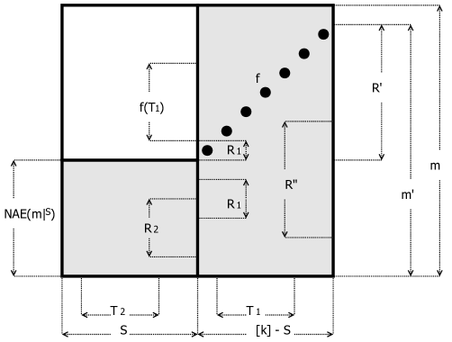
Figure 1: Argument for Theorem 4 (a). Upper-left region is white. Entries $(t,f(t))$ are not white.

Due to the maximality of $|S|$, there is no white rectangle on $\ell$ columns and $n-|S|-\ell+1$ rows inside ${\mathbf{m}}|_{[n]-\text{NAE}({\mathbf{m}}|^{S})}^{[k]-S}$ for any $\ell\geq 1$. That is to say, if we form a bipartite graph on right vertices corresponding to the columns $[k]-S$, and left vertices corresponding to the rows $[n]-\text{NAE}({\mathbf{m}}|^{S})$, with non-white cells being edges, then any subset of the right vertices of size $\ell\geq 1$ has at least $\ell+1$ neighbors within the left vertices.

By the induction on $k$ (since $S\neq\emptyset$), for the set of columns $[k]-S$ there is a set $R^{\prime\prime}$ of $k-|S|-1$ rows such that $\overline{{\varepsilon}}({\mathbf{m}}|_{R^{\prime\prime}}^{[k]-S})=-1$. Together with the rows of $\text{NAE}({\mathbf{m}}|^{S})$ this amounts to at most $k-2$ rows, so since $n\geq k$, we can find two rows outside this union; delete either one of them, leaving a matrix ${\mathbf{m}}^{\prime}$ with $n-1$ rows. This matrix has the rows $\text{NAE}({\mathbf{m}}|^{S})$ at the bottom, and $n-|S|$ remaining rows which we call $R^{\prime}$. The lemma will follow by showing that $\overline{{\varepsilon}}({\mathbf{m}}^{\prime})\geq-1$.

In ${\mathbf{m}}^{\prime}$, the induced bipartite graph on right vertices $[k]-S$ and left vertices $R^{\prime}$ has the property that any right subset of size $\ell\geq 1$ has a neighborhood of size at least $\ell$ in $R^{\prime}$. Applying Hall’s Marriage Theorem, there is an injective $f:[k]-S\to R^{\prime}$ employing only edges of the graph.

Now consider any set of columns $T$, $T=T_{1}\cup T_{2},T_{1}\subseteq[k]-S,T_{2}\subseteq S$. We need to show that ${\varepsilon}({\mathbf{m}}|^{T})\geq-1$. Let $R_{1}=\text{NAE}({\mathbf{m}}|^{T_{1}})\cap R^{\prime\prime}$, $R_{2}=\text{NAE}({\mathbf{m}}|^{T_{2}})\subseteq\text{NAE}({\mathbf{m}}|^{S})$, and note that $|R_{1}|\geq|T_{1}|-1$, $|R_{2}|\geq|T_{2}|-1$. If $T_{2}=\emptyset$ we simply use $R_{1}$. Likewise if $T_{1}=\emptyset$, we use $R_{2}$.

If both $T_{1}$ and $T_{2}$ are nonempty, $\text{NAE}({\mathbf{m}}|^{T_{2}})\subseteq\text{NAE}({\mathbf{m}}|^{S})$, and $|\text{NAE}({\mathbf{m}}|^{T_{2}})|\geq|T_{2}|-1$. Now use the matching $f$. The set of rows $f(T_{1})$ lies in $R^{\prime}$ and is therefore disjoint from $\text{NAE}({\mathbf{m}}|^{T_{2}})$. Moreover since $T_{2}\neq\emptyset$, every entry $(t,j)$ for $t\in T_{2},j\in R^{\prime}$ is white. On the other hand due to the construction of $f$, for every $t\in T_{1}$ the entry $(t,f(t))$ is non-white. Therefore every row in $f(T_{1})$ is in $\text{NAE}({\mathbf{m}}|^{T_{1}\cup T_{2}})$. So $|\text{NAE}({\mathbf{m}}|^{T_{1}\cup T_{2}})|\geq|T_{2}|-1+|T_{1}|$. Thus $\overline{{\varepsilon}}({\mathbf{m}}^{\prime})\geq-1$. ∎

4 From NAE to Rank: Proof of Theorem 4 (b)

Recall we are to show: 4 (b): $\mathbb{H}({\mathbf{m}})$ has full column rank if $\overline{{\varepsilon}}({\mathbf{m}})\geq-1$.

Proof.

The case $k=1$ is trivial. Now suppose $k\geq 2$ and that Theorem 4 (b) holds for all $k^{\prime}<k$. Any constant rows of ${\mathbf{m}}$ affect neither the hypothesis nor the conclusion, so remove them, leaving ${\mathbf{m}}$ with at least $k-1$ rows. Now pick any set, $C$, of $k-1$ columns of ${\mathbf{m}}$. By Theorem 4 (a) there are some $k-2$ rows of ${\mathbf{m}}$, call them $R^{\prime}$, on which $\overline{{\varepsilon}}({\mathbf{m}}|_{R^{\prime}}^{C})=-1$. Let $v$ be a row of ${\mathbf{m}}$ outside $R^{\prime}$. Call the rows of ${\mathbf{m}}$ apart from $v$, $R^{\prime\prime}$. Since $R^{\prime\prime}$ contains $R^{\prime}$, by induction $\dim\operatorname{Rowspace}\mathbb{H}({\mathbf{m}}|_{R^{\prime\prime}}^{C})=k-1$. Therefore $U:=\operatorname{Rowspace}\mathbb{H}({\mathbf{m}}|_{R^{\prime\prime}})\subseteq\mathbb{R}^{k}$ is of dimension at least $k-1$. We claim now that $\dim U=k$.

Suppose to the contrary that $\dim U=k-1$. If $v_{\odot}(U)\subseteq U$ then as proven earlier in Theorem 8, $U$ respects $B(v)$. Since $v$ is nonconstant, $B(v)$ is a partition of $[k]$ into $\ell\geq 2$ nonempty blocks $B(v)_{(i)}$, and $U=\bigoplus_{i=1}^{\ell}U_{(i)}$ with $U_{(i)}=P_{(i)}U_{(i)}$. So there is some $i_{0}$ for which $U_{(i_{0})}\subset V_{(i_{0})}$; specifically, $U_{(i)}=V_{(i)}$ for all $i\neq i_{0}$, and $\dim U_{(i_{0})}=\dim V_{(i_{0})}-1$. Since $|B(v)_{(i_{0})}|<k$, we know by induction that the rows of $\mathbb{H}({\mathbf{m}})$ span $V_{(i_{0})}$. Thus in fact $U=\mathbb{R}^{k}$. (Further detail for the last step: let $w\in\mathbb{R}^{k}$. Since the rows of $\mathbb{H}({\mathbf{m}})$ span $V_{(i_{0})}$, there is a $w^{\prime}\in\operatorname{Rowspace}\mathbb{H}({\mathbf{m}})$ s.t. $P_{(i_{0})}w^{\prime}=P_{(i_{0})}w$. Moreover since $U_{(i)}=V_{(i)}$ for all $i\neq i_{0}$, there is a $w^{\prime\prime}\in U$ s.t. $w^{\prime\prime}=(I-P_{(i_{0})})(w-w^{\prime})$. Then $w^{\prime}+w^{\prime\prime}\in\operatorname{Rowspace}\mathbb{H}({\mathbf{m}})$, and $w^{\prime}+w^{\prime\prime}=w$.) ∎

5 Motivation

Consider observable random variables $X_{1},\ldots,X_{n}$ that are statistically independent conditional on $H$, a hidden random variable $H$ supported on $\{1,\ldots,k\}$. (See causal diagram.)

The most fundamental case is that the $X_{i}$ are binary. Then we denote ${\mathbf{m}}_{i}^{j}=\Pr(X_{i}=1|H=j)$. The model parameters are ${\mathbf{m}}$ along with a probability distribution (the mixture distribution) $\pi=(\pi_{1},\ldots,\pi_{k})$ on $H$.

Finite mixture models were pioneered in the late 1800s in [13, 14]. The problem of learning such distributions has drawn a great deal of attention. For surveys see, e.g., [5, 17, 11, 12]. For some algorithmic papers on discrete $X_{i}$, see [9, 4, 7, 2, 6, 1, 15, 10, 3, 8]. The source identification problem is that of computing $({\mathbf{m}},\pi)$ from the joint statistics of the $X_{i}$. Put another way, the problem is to invert the multilinear moment map

$$\mu:({\mathbf{m}},\pi) \to\mathbb{R}^{2^{[n]}}$$

$$\mu({\mathbf{m}},\pi)_{S} =\Pr(X_{S}=1)\quad\text{ where }S\subseteq[n],\;X_{S}=\prod\nolimits_{i\in S}X_{i}$$

$$={\mathbf{m}}_{S}\cdot\pi^{\top}$$

The last line shows the significance of $\mathbb{H}({\mathbf{m}})$ to mixture model identification, since ${\mathbf{m}}_{S}^{j}=\Pr(X_{S}=1|H=j)$.

Connection to $\operatorname{rank}\mathbb{H}({\mathbf{m}})$.

In general $\mu$ is not injective (even allowing for permutation among the values of $H$). For instance it is clearly not injective if ${\mathbf{m}}$ has two identical columns (unless $\pi$ places no weight on those). More generally, and assuming all $\pi_{j}>0$, it cannot be injective unless $\mathbb{H}({\mathbf{m}})$ has full column rank.

One sufficient condition for injectivity, due to [16], is that there be $2k-1$ “separated” observables $X_{i}$; $X_{i}$ is separated if all ${\mathbf{m}}_{i}^{j}$ are distinct, or in our terminology, if no color recurs in ${\mathbf{m}}_{i}$. (Further [8], one can lower bound the distance between $\mu({\mathbf{m}},\pi)$ and any $\mu({\mathbf{m}}^{\prime},\pi^{\prime})$ in terms of $\min_{i,j}|{\mathbf{m}}_{i}^{j}-{\mathbf{m}}_{i}^{j^{\prime}}|$ and the distance between $({\mathbf{m}},\pi)$ and $({\mathbf{m}}^{\prime},\pi^{\prime})$.)

A weaker sufficient condition for injectivity of $\mu$, due to [8], is that for every $i\in[n]$ there exist two disjoint sets $A,B\subseteq[n]-\{i\}$ such that $\mathbb{H}({\mathbf{m}}|_{A})$ and $\mathbb{H}({\mathbf{m}}|_{B})$ have full column rank. (It is not known whether two disjoint such $A,B$ are strictly necessary, but the implied $n\leq 2k-1$ is in general best possible [15].)

References

- [1] A. Anandkumar, D. Hsu, and S. M. Kakade. A method of moments for mixture models and hidden Markov models. In Proc. 25th Ann. Conf. on Computational Learning Theory, pages 33.1–33.34, 2012.
- [2] K. Chaudhuri and S. Rao. Learning mixtures of product distributions using correlations and independence. In Proc. 21st Ann. Conf. on Computational Learning Theory, pages 9–20, 2008.
- [3] S. Chen and A. Moitra. Beyond the low-degree algorithm: mixtures of subcubes and their applications. In Proc. 51st Ann. ACM Symp. on Theory of Computing, pages 869–880, 2019.
- [4] M. Cryan, L. Goldberg, and P. Goldberg. Evolutionary trees can be learned in polynomial time in the two state general Markov model. SIAM J. Comput., 31(2):375–397, 2001. Prev. FOCS ’98.
- [5] B. S. Everitt and D. J. Hand. Mixtures of discrete distributions, pages 89–105. Springer Netherlands, Dordrecht, 1981.
- [6] J. Feldman, R. O’Donnell, and R. A. Servedio. Learning mixtures of product distributions over discrete domains. SIAM J. Comput., 37(5):1536–1564, 2008.
- [7] Y. Freund and Y. Mansour. Estimating a mixture of two product distributions. In Proc. 12th Ann. Conf. on Computational Learning Theory, pages 183–192, July 1999.
- [8] S. L. Gordon, B. Mazaheri, Y. Rabani, and L. J. Schulman. Source identification for mixtures of product distributions. arXiv:2012.14540, 2020.
- [9] M. Kearns, Y. Mansour, D. Ron, R. Rubinfeld, R. Schapire, and L. Sellie. On the learnability of discrete distributions. In Proc. 26th Ann. ACM Symp. on Theory of Computing, pages 273–282, 1994.
- [10] J. Li, Y. Rabani, L. J. Schulman, and C. Swamy. Learning arbitrary statistical mixtures of discrete distributions. In Proc. 47th Ann. ACM Symp. on Theory of Computing, pages 743–752, 2015.
- [11] B. G. Lindsay. Mixture models: theory, geometry and applications. In NSF-CBMS regional conference series in probability and statistics, pages i–163. JSTOR, 1995.
- [12] G. J. McLachlan, S. X. Lee, and S. I. Rathnayake. Finite mixture models. Annual Review of Statistics and Its Application, 6(1):355–378, 2019.
- [13] S. Newcomb. A generalized theory of the combination of observations so as to obtain the best result. American Journal of Mathematics, 8(4):343–366, 1886.
- [14] K. Pearson. Contributions to the mathematical theory of evolution III. Philosophical Transactions of the Royal Society of London (A.), 185:71–110, 1894.
- [15] Y. Rabani, L. J. Schulman, and C. Swamy. Learning mixtures of arbitrary distributions over large discrete domains. In Proc. 5th Conf. on Innovations in Theoretical Computer Science, pages 207–224, 2014.
- [16] B. Tahmasebi, S. A. Motahari, and M. A. Maddah-Ali. On the identifiability of finite mixtures of finite product measures. IEEE International Symposium on Information Theory (ISIT) 2018 and arXiv:1807.05444v1, 2018.
- [17] D. M. Titterington, A. F. M. Smith, and U. E. Makov. Statistical Analysis of Finite Mixture Distributions. John Wiley and Sons, Inc., 1985.