Data Analysis and Management (Computer Science and Engineering)

June 2020 May, 2020

Victor LempitskyAssociate Professor, PhD Yury MalkovPhD

TODOTODO, Skoltech

CNN with large memory layers

This work is centred around the recently proposed product key memory structure [46], implemented for a number of computer vision applications. The memory structure can be regarded as a simple computation primitive suitable to be augmented to nearly all neural network architectures. The memory block allows implementing sparse access to memory with square root complexity scaling with respect to the memory capacity. The latter scaling is possible due to the incorporation of Cartesian product space decomposition of the key space for the nearest neighbour search. We have tested the memory layer on the classification, image reconstruction and relocalization problems and found that for some of those, the memory layers can provide significant speed/accuracy improvement with the high utilization of the key-value elements, while others require more careful fine-tuning and suffer from dying keys. To tackle the later problem we have introduced a simple technique of memory re-initialization which helps us to eliminate unused key-value pairs from the memory and engage them in training again. We have conducted various experiments and got improvements in speed and accuracy for classification and PoseNet relocalization models.

We showed that the re-initialization has a huge impact on a toy example of randomly labeled data and observed some gains in performance on the image classification task. We have also demonstrated the generalization property perseverance of the large memory layers on the relocalization problem, while observing the spatial correlations between the images and the selected memory cells.

Chapter 1 Introduction

With the huge development of deep learning, neural networks have made significant progress in various tasks such as image classification [44], speech recognition [26], and machine translation [74]. As it was shown in [72, 54], with sufficiently large data, increasing the capacity of neural networks could lead to far superior prediction accuracy. Therefore, scaling of both training and model size has been a central problem of deep learning field in recent years. For a typical neural model where the single input data sample depends on all the parameters of the network, therefore increasing both dataset and model sizes leads to a nearly quadratic surge in the training costs [69].

Previous works [15, 12] proposed several ideas of increasing the model size with no proportional increase in a computational complexity. Most of the proposed models rely on the sparse gating mechanism which determines whenever a particular node of the graph should be calculated during the forward pass of the network. This is the type of a branching problem with a discrete decision which is being solved with REINFORCE algorithm [75]. It was applied in [8] and gave good results on MNIST dataset and CIFAR-10 [43] with a reasonable speed up.

Instead of REINFORCE estimator, one can also apply the ideas from [49, 34] by relaxing the discrete skipping decisions with reparametrization technique adoption. However, these approaches usually find sub-optimal solutions due to the approximation error introduced by the reparametrization trick [82, 1].

Other approaches rely on learning binary masks as the sparse $l_{0}$ regularization term for the final objective. Works like [53] employ a rectified sigmoid proposed in [48] to learn binary decision choices. Authors apply regularization during post-processing to quantize the weights of the network, but the idea could be used in the training phase too. Recently, the paper [58] on differentiable tabular data with neural networks has leveraged the entmax transformation [55] to learn ”hard” decisions for binary branching problem in decision trees.

Though solving the issue of scalability, models still fall short in giving promising results due to the following challenges:

• GPUs are optimized to work faster with arithmetic tasks rather than branching.

• Batching reduces the batch sizes for conditionally activated chunks, therefore complicating parallelization.

• REINFORCE estimator has a large variance, making it hard to get a strong bias during train. There are some variance reduction tricks [28, 51] that try to solve the issue but most of them skew the bias-variance trade-off with no tuning on hyperparameters applied.

• Nearly all the methods suffer from neuron dying problem - if at some moment of the training a gate is not open for any input sample, this means it is highly unlikely it will be open at any further moment since the gate receives only zero gradient.

A recent work [46] on the over-parametrized language models, on the other hand, rely on the key-value memory structures to scale the set of parameters in the neural network. Authors rely on the product key space decomposition for nearest neighbours to scale the networks with a little or no change in the performance and the memory consumption. These results encouraged us to research these methods in the computer vision applications.

As an extension of [46], we augment the product key layer with the key-value re-initialization mechanism which allows to solve the dying neuron problem. The mechanism is based on re-initialization of dead or underutilized keys-values pairs using the information from more successful key-values pairs.

Chapter 2 Related work

Memory layers in neural models Memory augmented neural networks (MANNs) augment neural networks with external memory block which allows for explicit access with differentiable write and read operations. The memory is usually implemented as a key-value differentiable dictionary [59], array-structured memory such as Turing machine (NTM) [27], or recently proposed product-key memory layers [46].

Key-value memory architectures were analyzed extensively in deep learning literature. Mostly the models are based on the architectural designs described in [73, 78] and used mainly in natural language processing field (NLP) such as document reading and question answering tasks. The key-value paired structure can be seen as a generalization of how the huge context for question answering is stored in the memory. That makes key-value memory a natural choice for these tasks. And with the recent advancements in attention models (AM) [5, 80], it is becoming the predominant concept in natural language processing literature with the usage case in nearly every NLP task.

The key-value design structure is a sparse version of attention models, and as previously described in [14, 7] the self-attention mechanism could be competitive in replacing convlolutions as a computation primitive for object detection and image classification. We hope to leverage and improve upon those ideas for computer vision applications.

There were also some works in extending the key-value structure, [25] using unbound cache model to provide better modelling of infrequent words that occur in a recent context, including the out-of-vocabulary words. This is the evidence of interpretability of learned key-value structure which provides the linear interpolation between the values of the table. Other works [39] focus on the interpretability of memory blocks by linearly interpolating baseline language models (LM) with k-nearest neighbours (k-NN) models and assessing the generalization and memorization capability of the final models. Authors report increased perplexity in all of the experiments.

Other approaches have successfully applied memory layers to store image features, more specifically for image captioning [13], image generation tasks [41], and video summarization [47].

Some neural network designs include non-differentiable memory layers with unsupervised updates. These models mostly rely on the architectural ideas of [89] and rely on contrastive loss to update the memory block. Authors of [89] have demonstrated the the efficiency of their memory block in few-shot and one-shot learning tasks, while [84] has shown the advantage of using the memory in style transfer [20] tasks with limited data. While in supervised approaches of memory usage where we are learning the mapping function between two spaces, in the unsupervised approach memory block is used for storing latent vectors with the ability to interpolate between them. This is the important property of memory blocks that is implicitly used in most of the models.

Some works incorporate memory-like structure to store a bank of weights accessing them sparsely and using k-nearest neighbours to retrieve a set of indices that allows to encode the feature vector into the discrete code. There are some promising results in auto-regressive models [79] giving high-fidelity image reconstruction results in [63]. Authors argue that the discrete representation is a more natural fit for complex reasoning, planning and predictive learning.

Moreover, memory layers were successfully incorporated in graph knowledge representation problems, with promising results in graph classification tasks [40].

Learning compact representations, ANN. Since the task of exact top-k neighbour search is expensive in practice for high dimensional embeddings, i.e. linear scale to the search set size, practitioners in the field usually resort to more scalable approximate nearest neighbours methods (ANN). Popular methods include Locality sensitive hashing (LSH) [22, 2] that relies on random space partitioning, graph methods like Navigable small world graphs (NSW) [50] and Hierarchical NSW (HNSW) [6] based on constructing the search algorithm by finding the clusters of data. Another important subset of methods utilize quantization [21, 18, 4] to reduce the memory consumption and speed up the distance calculations. Many of those methods exploit the idea of product decomposition, e.g. assumption that the space can be decomposed into a Cartesian product of low dimensional spaces.

Product decomposition in neural models Most of this thesis is inspired by the work of [46] which are showing the efficiency of using product key memory layer in language modelling tasks. Here product key is a structure that allows more efficient scaling by scarifying some expressiveness of the model. Authors find that the language model augmented with memory with only 12 layers can outperform in accuracy a baseline transformer model with 24 layers while giving two times less inference time. The [46] didn’t however address the problem of dying keys other than by adding noise to the query (via batchnorm) and was focused solely on NLP applications.

Product quantization in general has also been used in many computer vision applications, starting from scalable supervised [56] to semi-supervised [35] image retrieval tasks. There are some promising results [83] in face video generation with memory augmented Generative adversarial networks (GAN) [23].

Classification networks Huge chunk of work [76, 30, 45, 70] is done in designing the neural networks for the image classification problems. In our experiments we mainly focus on the ResNet-like [30] networks. Some recent work [77] demonstrated the SOTA results in ImageNet-2012 dataset [44] with the help of the reinforcement learning to tune the models and the whole architecture. Most of the existing neural networks for image classification rely on the convolutional block but there were some recent works suggesting the self-attention mechanism with promising results [7, 62].

Chapter 3 Methods

3.1 Product key memory

3.1.1 Design overview

The overall pipeline of the differentiable product memory layer is similar to most of the key-value data structures that are augmented into neural network models [27, 78, 73]. More specifically, product memory design in our work is heavily inspired by previously proposed architecture in [46]. Here we build models upon this design to solve classification, regression, and reconstruction computer vision tasks.

Higher view of the architecture is illustrated in Figure 3.1. The central idea is to augment baseline convolutional neural networks with sparse memory access. The input of the memory layer is the latent feature vector that describes the given input image. Depending on where we place the memory layer, the query can represent features like brightness gradients or colours with more complex patterns in later layers [87]. Therefore, the choice of memory access placement is important. Given the input query, memory block finds the distance scores by comparing it with all of the keys in the table and selecting the values associated with top-k distance scores. The scores are then used to produce the output $m(x)$ via a weighted sum over the values associated with the selected keys:

$$m(x)=\sum_{i\in\mathcal{I}}w_{i}v_{i}$$

where $\mathcal{I}$ is the set of top-k indices by distance scores, $w_{i}$ are the scores, and $v_{i}$ are the values in the memory layer.

Query generation. The memory block consists of the query generation network which is a learnable projection function $q:x\rightarrow q(x)\in\mathbb{R}^{d_{q}}$ mapping the d-dimensional input vector x into the $d_{q}$-dimensional query vector. Typical dimension sizes of the query vectors in our experiments are from 256 up to 2048.

Also, since the keys are initialized in a fixed range, we follow [46] adding BatchNorm [33] layer on the top of the query network. This allows a better overlap between the distribution of keys and queries. And as in [46] we observe higher utilization of the memory with BatchNorm enabled.

Key assignment We have a resulting query $q(x)$ that should be assigned to the closest keys with the selected metric for the distance. Let $\mathcal{K}=\{k_{1},\ldots,k_{|\mathcal{K}|}\}$ is the set of all keys, the set is composed of $|\mathcal{K}|$ $d_{q}$-dimensional vectors that are uniformly initialized in the $\mathbb{R}^{d_{q}}$ space. We can define the differentiable procedure to find a weighted sum over the value vectors (the memories associated with top-k keys). The sum is weighted by the distance scores between the subset of the top-k keys and the query value $q(x)$. Top-k procedure finds the most closest keys to the given query, i.e. maximization of the chosen similarity measure $d(\cdot,\cdot)$. The overall algorithm is:

$$\mathcal{I}=\mathcal{T}_{k}\left(d(q(x),k_{i})\right)$$

$$w=\operatorname{softmax}\left(\left\{d(q(x),k_{i})\right\}_{i\in\mathcal{I}}\right)$$

$$m(x)=\sum_{i\in\mathcal{I}}w_{i}v_{i}$$

where $\mathcal{T}_{k}$ denotes the top-k operation which finds k largest values based on the similarity measure $d(\cdot,\cdot)$. $\mathcal{I}$ denotes the index set of the most similar keys to the query $q(x)$ and $w$ represents the normalized scores associated with the selected indices. The resulting value $m(x)$ is the sum of the selected values weighted by the normalized scores. As we see due to the summation over the normalized values in the $\operatorname{softmax}$ operation, the gradients can be calculated. Note that it is not possible to find the gradient for top-1 function, since there is no summation.

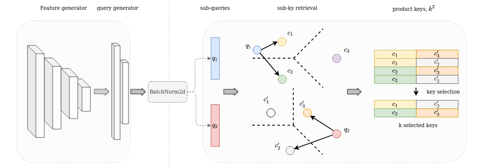
Figure 3.1: Overview of the product key-value memory design. Feature generator is the baseline image model which outputs the latent vector that is projected by the the query generator, normalized and divided into the two sub queries $q_{1}$/$q_{2}$ to work with product key values. As the result we have k selected keys and the corresponding values from $\mathcal{V}$.

Product keys We see that the bottleneck of the given procedure is the calculation of the $\mathcal{T}_{k}$ the operation which has linear complexity over the size of the key set $\mathcal{K}$, so it is hard to scale this procedure for large memory sizes. The remainder of operations are done for the reduced set of selected indices, e.g. the summation over top-k normalized weight values.

To solve the performance issue, authors of [46] propose to represents the key set in the form of two independent sets of half dimension size $d_{q}/2$ vector sets $\mathcal{K}_{1}$ and $\mathcal{K}_{2}$ which constructs the Cartesian product set of resulting values with size $|\mathcal{K}|=|\mathcal{K}_{1}|\times|\mathcal{K}_{2}|$. The query vector should also splitted into two sub-queries $q_{1}$ and $q_{2}$ to work in each of the key sets. We then find the closest keys in both sets as:

$$\mathcal{I}_{\mathcal{K}_{1}}=\mathcal{T}_{k}\left(\left\{d(q_{1}(x),k_{i}^{1})\right\}_{i\in\{1\ldots|\mathcal{K}_{1}|\}}\right),\quad\mathcal{I}_{\mathcal{K}_{2}}=\mathcal{T}_{k}\left(\left\{d(q_{2}(x),k_{j}^{(2)})\right\}_{j\in\left\{1\ldots\left|\mathcal{K}_{2}\right|\right\}}\right)$$

Then the two subsets of the keys associated with the index sets $\mathcal{I}_{\mathcal{K}_{1}}$ and $\mathcal{I}_{\mathcal{K}_{2}}$ are multiplied together to form a new Cartesian product set. We are applying the top-k operation on the newly created set and find the final subset of the top-k keys.

Choice of distance Authors in [46] experiment with the inner product as the single similarity measure for the provided experiments. We observe that using cosine similarity not only provides us with better numbers in some experiments but also gives us control over the selection process of the keys. Since the dot product is proportional to the vector norm, the key vectors with the largest vector lengths will be selected in most of the cases, while low norm vectors may be completely ignored. This means that the distance measure captures the most popular candidates, the latter can skew the similarity metric. We balance the skew by introducing the hyperparameter $\alpha$ and raising the length to an exponent $\alpha<1$ to calculate the distance as:

$$d_{cos}(q,k,\alpha)=|q|^{\alpha}|k|^{\alpha}\cos(\theta)=|q|^{\alpha}|k|^{\alpha}\frac{q^{T}k}{|q|\cdot|k|}$$ (3.1)

Multi-head mode To make the model more expressive we are using the multi-head mechanism [80] which splits queries and keys into multiple chunks of vectors to be calculated independently. The similar calculations are conducted on each head and the results are concatenated. Due to the reduced dimension of each head, the overall computational complexity of the layer is similar to the single-head attention.

Complexity Naive top-K key selection requires $\mathcal{K}$ comparisons of $d_{q}$ sized vectors, which gives us $\mathcal{O}\left(|\mathcal{K}|\times d_{\mathrm{q}}\right)$ operations overall. When using the product space $\mathcal{K}=K_{1}\times K_{2}$, we have two separate sets of keys for subspaces with significantly reduced carnality $|K_{1}|=|K_{2}|=\sqrt{|\mathcal{K}|}$. The overall complexity for the first step then is: $\mathcal{O}\left(|K_{1}|\times d_{q}/2+|K_{2}|\times d_{q}/2\right)=\mathcal{O}\left(|K_{1}|d_{q}\right)=\mathcal{O}\left(\sqrt{\mathcal{|K|}}d_{q}\right)$. The second step is performed on the reduced subset of $k\times k$ elements so it will require $\mathcal{O}\left(k^{2}\times d_{1}\right)$ operations. Therefore overall complexity is:

$$\mathcal{O}\left(\left(\sqrt{|\mathcal{K}|}+k^{2}\right)\times d_{\mathrm{q}}\right)$$

3.2 Re-initialization trick

3.2.1 Overview

While conducting our initial experiments on random data, we have observed that a toy neural network augmented with memory block struggles to fit the data with no multi-head mode enabled even though the model should have had enough capacity to fit the whole dataset. By conducting some ablation study and literature review [3] we have concluded that the problem is due to the correct initialization of the memory layer. Additionally, authors in [81] suggest that most of the heads in the attention mechanism can be pruned without serious effect on the performance. To tackle the initialization issues we are introducing the re-initialization trick that dynamically initializes unused keys during the training phase. We are describing the whole procedure below.

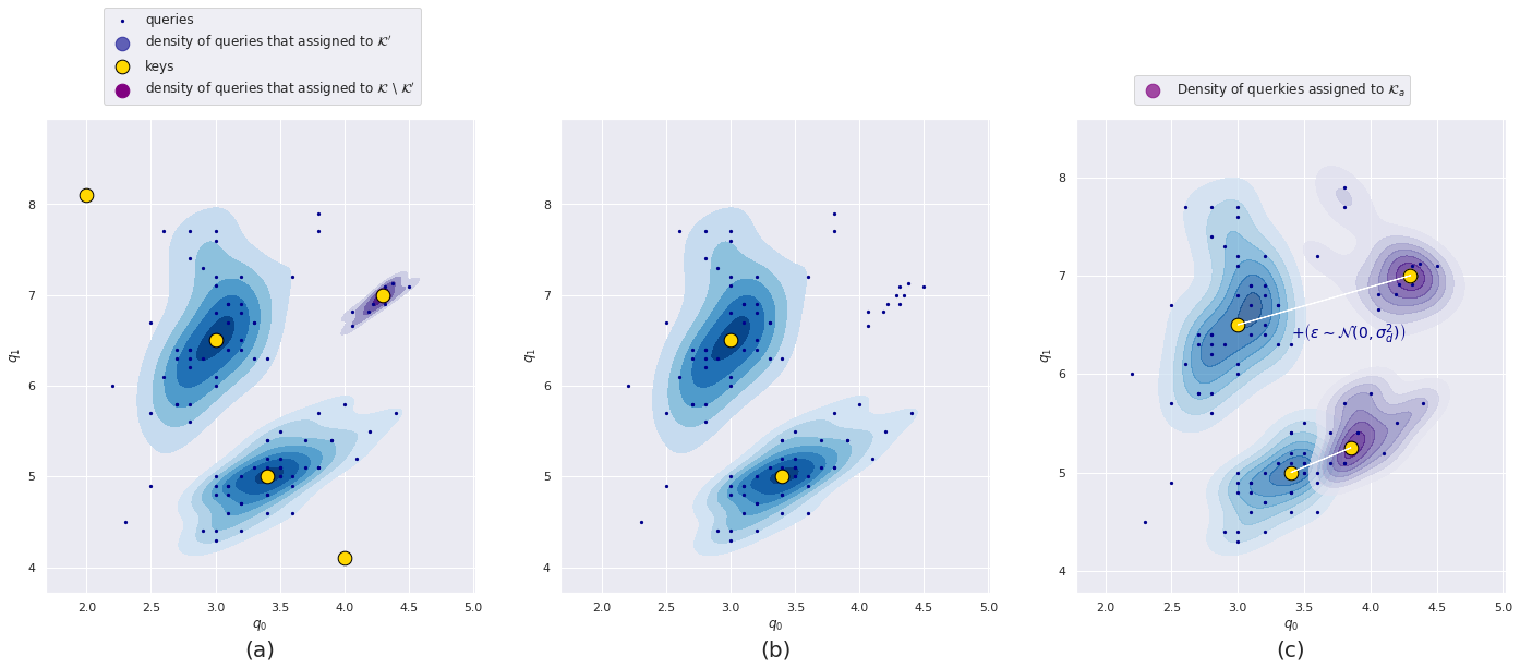
Figure 3.2: The illustration of the key re-initalization procedure. (a) We have 5 keys with three of which does not pass the threshold of being identified as the ”utilized keys”. We are removing those keys in the step (b). And in the step (c) we are initializing new keys sampled from existing ones and perturbed with an additive Gaussian noise ($\epsilon\sim\mathcal{N}(0,\sigma_{d}^{2})$).

3.2.2 Problem of dying keys

Let’s assume that we are working with the dataset of size $|\mathcal{D}|$ which is equal to the number of values in the memory $|\mathcal{M}|$. We could assume that augmenting the neural network with the memory layer could lead to the full convergence, i.e. perfect accuracy, because of the one-to-one mapping between the input and the memory elements. We hovewer did not observe this in our experiments with random data (description is in the experiments section), and classification tasks. Instead, we discover continuously reduced cardinality of the selected key set at each iteration of the optimization, reaching some fixed value $|\mathcal{K}^{\prime}|$:

$$|\mathcal{K}^{\prime}|=\alpha|\mathcal{K}|,\,\alpha\ll 1$$ (3.2)

$$\mathcal{K}^{\prime}=\left\{k_{i}\in\mathcal{K}|c_{i}>0,c_{i}\in\mathcal{C}\right\}$$ (3.3)

where $K^{\prime}$ is the set of selected keys during the inference, $\mathcal{K}$ is the set of all keys, and $c_{i}$ is the utilization of the key $k_{i}\in\mathcal{K}$ summed for the whole dataset, i.e. number of times the key $k_{i}$ was selected. In the experiments we are not able to get full utilization of the selected keys and observed low final accuracy. We call this a problem of dying keys, when the optimizer is unable to pass gradients through certain key-value pair in the memory layer, leading us to the dead keys, useless for inference but still having a computational burden.

3.2.3 Key re-sampling

To solve the problem we implement a simple trick of key re-initialization, which is being executed during the training phase at certain points. We observe that during training, the key utilization converges to some specific number, as it is given in Equation (3.2). We assume that the main reason for this is dying keys problem discussed in the previous section. For this reason, we are running the pipeline of key re-initialization when the utilization plateau is reached.

Here we describe the algorithm for a single product space key subset but the algorithm is applicable for both of key subsets. Let $\mathcal{K}$ define the set of all the keys in memory and $\mathcal{K^{\prime}}$ is the subset of utilized keys where $|\mathcal{K^{\prime}}|\ll|\mathcal{K}|$. We also introduce the hyperparameter $k_{a}$ which will control how many keys should be re-sampled at the each call of our key initialization procedure. Then we have:

$$\mathcal{I}_{a}=\left\{i|i\sim U\{0,|\mathcal{K}^{\prime}|\}\right\}$$

$$\mathcal{K}_{a}=\left\{k_{i}\in\mathcal{K}^{\prime}|i\in\mathcal{I}_{a}\right\}+\epsilon,\epsilon\sim\mathcal{N}(0,\sigma_{n}^{2})$$

$$\mathcal{K}=\mathcal{K}_{a}\cup\mathcal{K}^{\prime}$$

where $\mathcal{I}_{a}$ is the set of indices sampled uniformly from the used keys $\mathcal{K}^{\prime}$, $\mathcal{K}_{a}$ is the sampled set of utilized keys perturbed with guassian additive noise. We have an additional hyper parameter $\sigma_{n}$ that controls the noise variance of the re-initialized keys, i.e. the magnitude of difference between the original keys and re-initialized ones. Then the existing set of utilized keys are expanded by $\mathcal{K}_{a}$. The sampling mechanism we discussed above is very basic, but sampling more from the regions of high density/low density could potentially bring us more gain both in prediction accuracy and the compactness of the final representation. This, however, requires the re-initialization algorithm to be able to sample key points in the regions with higher density. Something like rejection sampling algorithms, i.e. Metroplolis-Hastings algorithm [66] could save us here, by defining the multimodal normal distribution and the utilization of the key values as the mean parameter. But because of the difficulty of tuning the rejection sampling algorithm, we plan to test those algorithm in the future and resorting to simple re-sorting discussed in the following section.

3.2.4 Re-sorting and key-value reinititalization

To give more priority on the regions of high density during sampling, we are sorting the keys in the set by the utilization coefficients $c_{i}\in\mathcal{C}$, and adapting a naive thresholding logic to eliminate the least utilized keys by removing those with the values less than the hyper parameter $d_{k}$ Then the index set calculated is:

$$\mathcal{K}_{d_{k}}=\left\{k_{i}\geq d_{k}|k_{i}\in\mathcal{K}\right\}$$

$$\mathcal{I}_{a}=\left\{i\in\{0..|K|\}|k_{i}\in\mathcal{K}_{d_{k}}\right\}$$

After we resample the keys by eliminating the least utilized, we to initialize new values $\mathcal{U}_{a}$ that will be mapped to the elements of the Cartesian product set of the new keys $\mathcal{K}_{a}$. Because of the set product, adding single key to the subset will add $|\mathcal{K}_{a}||\mathcal{K}|$ new values into the memory. For each key from the first product set, we are initializing new values associated with the resulting keys concatenated with the given key from the first set and all the existing keys in the second set. The same applies to the values associated with the second product set. The overall algorithm for the re-sampling step is demonstrated in Algo 1.

Algorithm 1 Re-initialization algorithm

1:existing set of keys $\mathcal{K}^{\{0,1\}}$, noise variance $\sigma_{n}$, utilization set $\mathcal{C}^{\{0,1\}}$, threshold parameter $d_{k}$, and the weight values $\mathcal{U}$

2:Reinitialized set of keys $\mathcal{K}$, Reinitialized values $\mathcal{U}$

3:function keysort($\mathcal{K},d_{k}$)

4: $\mathcal{K}_{d_{k}}=\left\{k_{i}\geq d_{k}|k_{i}\in\mathcal{K}\right\}$

5: return $\mathcal{K}_{d_{k}}$

6:end function

7:for $j\in\{0,1\}$ do

8:   $\mathcal{K}_{d_{k}}^{j}=\operatorname{keysort}(\mathcal{K}^{j},d_{k})$

9:   $\mathcal{U}=\mathcal{U}\setminus\left\{\mathcal{U}_{i}|i\in\left(\mathcal{K}^{j}\setminus K_{d_{k}}^{j}\right)\times\mathcal{K}^{(-j)}\right\}$

10:   $\mathcal{I}_{a}^{j}\sim U\left\{i\in\{0..|\mathcal{K}^{j}|\}|k_{i}\geq\mathcal{K}^{j}_{d_{k}}\right\}$   sample $a$ indices from the discrete distribution

11:   $\mathcal{K}_{a}^{j}=\left\{k_{i}\in\mathcal{K}^{j}|i\in\mathcal{I}_{a}^{j}\right\}+\epsilon,\epsilon\sim\mathcal{N}(0,\sigma_{n}^{2})$

12:   $\mathcal{K}^{j}=\mathcal{K}^{j}_{a}\cup\mathcal{K}^{j}_{d_{k}}$

13:   $\mathcal{U}^{\prime}=\left\{u_{i}^{\prime}\sim U|i\in[0..|\mathcal{K}_{a}^{j}||\mathcal{K}^{-j}|]\right\}$

14:   $\mathcal{U}^{j}=\mathcal{U}^{j}\cup\mathcal{U}_{a}^{j}$  We need to associate the indices of newly created values with keys

15:end for

16:$\textbf{return}\,\mathcal{K}^{\{0,1\}},\mathcal{U}$

3.2.5 Re-initialization complexity

Taking the constant complexity of random number generation we can assume that the index sampling from discrete distribution is also constant. Then the complexity of key generation for both subsets is $\mathcal{O}(d_{q}\times|\mathcal{K}_{a}|)$. The complexity for value re-sampling is $\mathcal{O}(|\mathcal{K}_{a}|\times|\mathcal{K}|\times d_{1})$ which in result give us the complexity of the whole procedure as:

$$\mathcal{O}(d_{q}\times|\mathcal{K}_{a}|)+\mathcal{O}(|\mathcal{K}_{a}|\times|\mathcal{K}|\times d_{v})$$

where $d_{v}$ is the dimension of the memory value vectors.

3.3 Classification pipeline

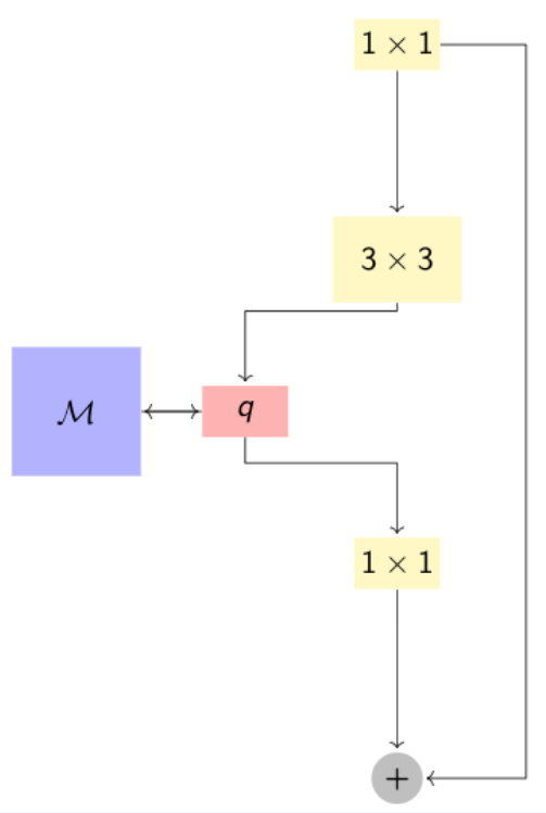
Figure 3.3: Bottleneck [30] augmented with a memory block $\mathcal{M}$.

We are augmenting various types of the classification neural networks with the memory layer defined in the sections above. ResNet [30] is the baseline architecture for most of the experiments. The first idea is to augment the Bottleneck block with the memory layer. The memory is inserted after the ($3\times 3$) kernel size convolution layer. We could also add the memory access before the middle convolution layer but we didn’t find any differences between the two methods so we just stick with the first design. We are keeping the baseline high-level architecture the same by only replacing the single Bottleneck block with the augmented version. Replacing a single layer should be enough to observe the effect of the memory, while having only a single layer with relatively low spatial size allows less carrying about the efficiency of the layer implementation.

Inspired by [32] we are also adding the memory access in squeeze-and-excitation (SE) like manner. SE is a computation block that can be built upon any transformation in the network. It consists of two parts. First, Squeeze which, given the feature map, captures the global spatial information and squeeze it into the channel descriptor. Authors use global average pooling with that goal. Second, Excitation, which employs the simple gating mechanism upon the projection of squeezed vector with a sigmoid activation. The projection is the bottleneck with two fully connected layers around the non-linearity. The bottleneck layer successfully limits the complexity of the SE block by introducing the dimensionality-reduction with ratio $r=d_{in}/d_{out}$, where $d_{in}$ is the dimension size of input vector and $d_{out}$ is the dimension size of the vector after the first projection in the bottleneck.

We setup nearly the same design but with three main differences, first, we are replacing only one block instead of every/several blocks in [32] (fewer SE blocks give worse final score). This reduces the number of parameters to be stored in the memory and the overall FLOPS required in the inference. Second, channel-wise feature response is fed to the memory instead of the MLP with two fully-connected (FC) layers around the non-linearity. This design helps us to tackle the issues of large spatial shapes of the query input and therefore softens the overall performance drop. Finally, instead of re-scaling the values of the feature map with the gating output, we are simply adding the embedding pixel-wise, i.e. replacing multiplication by addition operation and adding the embedding to each pixel of the feature map. The overall model of memory augmented squeeze-and-excitation block is illustrated in Figure 3.4.

Another option is to simply add the memory block as an additional layer between the existing ones. This way we still have the issues with large spatial shapes, especially for the earlier layers. We are testing this design type with the ImageNet dataset [44].

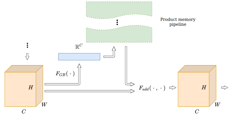
Figure 3.4: The overview of the modified squeeze-and-excitation block augmented with the memory layer. $F_{GB}$ is the function of global pooling which reduces the dimension of 3 dimensional feature map to the signle dimension, and $F_{add}$ is channel-wise addition of a resulting vector from memory to the original feature tensor.

3.4 Regression pipeline

To test the capability of the memory layer to work on regression problems, we are also experimenting with the camera relocalization problem [38]. The task is to find the camera extrinsics, i.e. the camera’s location in the real world and its direction, from the single image. Inferring the camera extrinsics is a crucial task for mobile robotics, navigation, augmented reality.

Authors of the PoseNet neural network [38] construct the simple neural model which consists of the backbone network and two additional layers that map the feature representation of the input into the pose and the direction values. First, it is the regression feature generation network as a basis for the architecture. For that purpose GoogleNet [76] is used, we are replacing it with ResNet [30] to conduct our experiments. The output of the backbone is fed to the fully connected layer, which is then regressing values for direction and orientation separately. Authors of the paper suggest to parametrize the direction with quaternions because of the overall simplicity compared to the rotational matrice, i.e. advantage in size: 4 scalars vs 9 in rotation matrix and speed since quaternion multiplication is much faster compared to a matrix-vector product used for rotation matrices. Additionally, since the rotation matrices $n\times n$ are the members of $SO(n)$ [37], they have the orthonormality property that should be preserved during the optimization, which is generally the hard problem.

Since quaternion, q, is identical to -q, this leads us to the issue of non-injectivity of the rotation value. To solve it authors normalize a quaternion rotation to a unit length:

$$\mathcal{L}_{q}(I)=\left\|\mathbf{q}-\frac{\hat{\mathbf{q}}}{\|\hat{\mathbf{q}}\|}\right\|$$

For position loss, $L_{2}$ Euclidean norm is used. Introducing scaling factor $\beta$, we can balance the overall loss, by keeping expected values of two losses approximately equal. We are not trying to tune the scaling factor in our experiments since it is not the main direction of this research, but we still experiment with a large grid of hyperparameters including various values for the scaling factor. The overall objective loss function is:

$$\operatorname{loss}(I)=\|\hat{\mathbf{x}}-\mathbf{x}\|_{2}+\beta\left\|\hat{\mathbf{q}}-\frac{\mathbf{q}}{\|\mathbf{q}\|}\right\|_{2}$$

We are experimenting with memory block by replacing the fully connected layer before the final regressor of feature size 2048. Since the data size (King’s College [38]) on which the experiments are conducted is relatively small, we are constraining ourselves with setting the memory size to 1k/10k values. We also regularize the memory layer by augmenting weights with Dropout (multiplicative binomial noise) but find far worse results.

3.5 Image reconstruction pipeline

To test the memory layers further we are working with an image reconstruction problem on the Imagenet-2012 [44] dataset. Image reconstruction is the type of dimensionality reduction problem to learn the projection function that could inject the given image into the latent representation in the compact manifold (data encoding) and then generate the image from the given latent. Autoencoder is a neural approach that helps us to tackle the problem in an unsupervised fashion. In the basic design of the autoencoders, we have two networks: encoder which maps the image into the small latent code and a decoder which generates the image from the code.

We are experimenting with several autoencoder designs but stick to: DCGAN [60] generator as the decoder network and the encoder as the custom 2D neural network consisting of five ResNet blocks. The image latent is the 1024 dimensional vector. The architectural choice of the augmentation is described in the section about the classification pipeline. We are using the basic method of augmentation by inserting an additional memory layer in the decoder network.

We observe that the location of the memory layer is important on how the memory is utilized on the train/validation sets and the final reconstruction results.

Chapter 4 Experiments

4.1 Experiments on random labels

The heart of our methodology to test the memory layers and re-initialization technique is a well-known variant of randomized test in non-parametric statistics [19, 88]. Drawing motivation from [88] we have conducted several experiments to test the ability of our memory layer to fit the randomly labelled set of data points. For this reason, we have prepared a simple data set with $N$ sample points. We are regulating the number of samples to much the memory size $M$. This is because our goal was having the one-to-one correspondence between the input data and the memory values, i.e. ideally overfitted memory layer. Sample points are the vectors uniformly generated in $\mathbb{R}^{8}$ space, i.e. points in 8 dimensional cube. There are a total of $m$ classes that are uniformly chosen for each data point. We have experimented with the data set of 100k data points with 10 classes, consequently setting $|\mathcal{M}|$ to 100k also.

Architecturally we have limited ourselves with the simplest model design with two linear projections before and after the memory layer. It is the basic architecture we could think of with no convolutional neural networks involved. Moreover, we observe that using convolutional layers allows us to fit the model to the dataset ideally. There is some research on the connection between the multi-head self-attention and convolutional layers [14], so we have tried to avoid the ambiguity and focused on the fully connected layers as the projections in our network.

Also to compare our key-value structure with classic dense layers, we have replaced memory access with very wide linear layers and point-wise non-linearity, i.e. ReLU, sigmoid. As it is described in [11], wide layer networks are a powerful memorizers, though in [86] authors are able to get great memorization for small ReLU networks also, with some initialization technique for SGD [64]. So it was interesting to see how the key-value structure memorization capability can be compared with the wide dense layers. We have used two fully connected layers with the ReLU in the middle. The weight matrix of the layers are set to project the 512-dimensional vector to the $\mathbb{R}^{15k}$ space and after applying the nonlinearity, acting as the discriminant function in the feature space divided by hyperplane decision surfaces, we are projecting the vector back to the space $\mathbb{R}^{512}$. This network of two projections and the nonlinearity in the middle is the approximation of our memory layer. This is because the k-nn function also acts as the discriminator function, more on this in [24] (Chapter 12).

We have trained our models with an Adam optimizer [42], with an initial learning rate of $10^{-3}$, and $\beta_{1}=0.9$, $\beta_{2}=0.98$. The models were implemented in Pytorch [57]. For the memory values we have chosen the SparseEmbedding structure which calculates and stores only the sparse gradients in the backward. We have chosen the SparseAdam (implemented in Pytorch) to update the sparse gradients in the memory layer. Because of the sparse updates in the memory, we have multiplied the learning rate for the sparse parameters by the factor of 10. For key parameter update, we have used the same optimizer as for the dense parameters. Due to the usage of re-initialization trick and Adam optimizer which stores the values of past gradients and square gradients, these values should also be dynamically updated. The results for the models with memory blocks and wide dense layers compared in Figure 4.1.

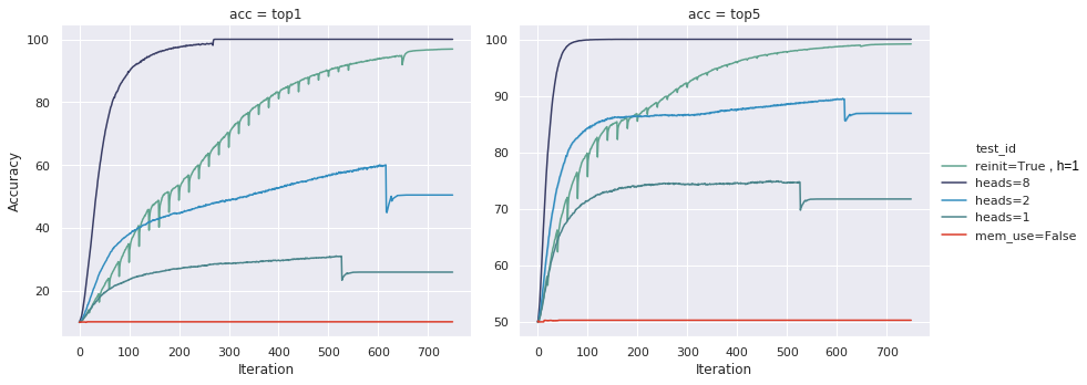
Figure 4.1: Results for the random data on the various models. The left graph is the plot for top-1 validation accuracy results, top-5 is pictured on the right. We can see that the model with no memory is not able to fit the data. Setting 8 heads for multi-head attention memory model, on the other hand, helps the model to easily fit the data. Re-initialization helps to get nearly full convergence with on only 1 head, i.e. multi-head mode disabled. Also, $h=1$ in the graph is the notation for the single head model.

In our experiments, we varied the hyper-parameters of the memory model, such as memory size, number of heads, k parameter in top-k operator, etc. We provide the results only for {$k=10$, $N=M$} hyperparameter set with different values for the number of heads $h$ and the re-initialization trick enabled/disabled since other combinations contain no interest in these experiments.

We observe that setting the number of heads to 8 gives us perfect fit to the data, i.e. full top-1 validation accuracy. As it is shown in Figure 4.1, replacing the memory layer with wide dense layer doesn’t help us with the accuracy. Lowering the number of heads, we see the declining accuracy in the validation. We speculate that this is caused by the poor initialization due to which the pair of the same keys could be selected for the two very close query vectors. Using uniform initialization to maximize the key coverage at the initial state of the model didn’t help us to resolve the issue as we have observed that the utilization of keys converged to some small subset.

To overcome the problem, we have experimented with re-initialization trick that was introduced in the chapter above. As it is seen from Figure 4.1, re-initialization helps us to get nearly ideal validation accuracy even with a single head. We are setting $\epsilon_{d}=10^{-6}$ to get the results above. We haven’t experimented much with the special scheduler for the re-initialization trick, but early experiments showed that the frequency with which the re-initialization procedure is called and the number of added keys for each call can have the significant influence on the final accuracy we get. More experiments are required in this direction.

We have conducted some additional experiments to see how the variance $\sigma_{d}$ parameter of the additive noise added to the re-initialized keys and the memory values affect the final accuracy. We are giving the results in in Figure 4.2

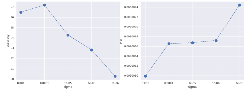
Figure 4.2: Relation between $\sigma_{d}$ hyper parameter of the Gaussian noise square variance parameter in re-initialization procedure and the values of train accuracy and loss for the random data. Setting higher $\sigma_{d}$ helps significantly, giving lower loss.

4.1.1 Results on CIFAR-10

We have implemented several architectural ideas to test the performance of memory augmented models on CIFAR-10 [43]. The first idea was to augment the bottleneck blocks [30] with the memory layer and replace the single bottleneck in the network with the modified block. We have also experimented with replacing multiple bottlenecks blocks but didn’t find anything reasonable to stick with it in the experiments because of the overall increased inference time we have observed.

The logic behind the bottleneck augmentation is given in the chapter above. Here we describe the architectural choices we’ve made to incorporate the augmented bottleneck in the most optimal way possible taking into consideration the inference time and the final validation accuracy. The real hurdle during the experiments was the speed issues of the inference. It didn’t allow us to set up experiments with more broader set of models because of the time limitations and the general difficulty of running large grids rapidly for slower models. We were able to partly mitigate the issues by using a lower spatial size of the query input. Taking all this into the consideration, we have chosen the last layer to be augmented with the memory layer as it gave us the smallest spatial size possible in the ResNet-type network. We have abandoned the experiments with larger spatial sizes in classification experiments for CIFAR-10 since the balance between the performance and the accuracy wasn’t reasonable. But we still have conducted experiments with larger spatial sizes with the autoregressive models, the results are available in the sections below.

We have chosen the ResNet-50 [30] to be the baseline network for the experimental models. The baseline consists of two projections and 16 Bottleneck blocks in the middle. We have added the memory layer in the 14th Bottleneck block and have illustrate the results in Figure 4.3. The training loop design described in [30] have been implemented with the SGD [65] optimizer, learning rate of $10^{-1}$ weight decay of $0.0001$ and momentum equal to $0.9$. Since the model contained the sparse parameters, we weren’t able to use the standard implementation of the SGD optimizer in PyTorch [57]. For that, we have implemented the SparseSGD optimizer with disabled weight decay. As for the momentum, to our knowledge, there is no mathematical ground of using it to accelerate sparse gradients, but we have still set it to 0.9 in all of our experiments. More information on the sparse SGD can be found here [17].

We have adopted the weight initialization as in [29] and the batch normalization (BN) [33]. The augmentation is the same as in [30] with 4-pixel padding on each side of the image and 32$\times$ 32 crop randomly sampled from the padded image and random horizontal flip. All of the experiments have been conducted with the memory size of 100k, top-k operator parameter k of 30 and no dropout on the retrieved indices applied. Setting the memory size to 100k we have two sets of product keys of size 100, $|\mathcal{K}_{1}|=|\mathcal{K}_{2}|=100$.

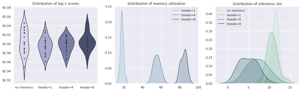
Figure 4.3: Comparison of the top-1 scores, memory utilization and the inference speed for the model with no memory augmentation and three memory augmented models with the number of heads in the set of {1, 4, 8}. There are 20 runs for the each experiment with the different initial seeds. As it can be observed, there is no evident increase in the accuracy while the performance of the models with the heads is much worse compared to the baseline models. Inference values are calculated on GTX-1080Ti cards with fp32 mode, the results are approximate.

We have calculated the distributions of top-1 scores for 20 runs with different seed values. As it is seen in the Figure 4.3 we weren’t able to gain any improvements in the accuracy scores with the memory augmentation, while the performance of the memory model, i.e. iterations per second in the train, decreases significantly and continues to decrease with the higher number of heads. We have also calculated the distributions of the memory utilization and observed that for larger heads we see the increase in the overall utilization. These findings mirror the results in [46].

Evaluation metrics for memory layer. As the simple evaluation metric of how well the memory is being utilized during the training phase, we have calculated the memory usage score which represents the fraction of accessed values $\#\{\mathcal{C}_{i}\neq 0\}$, where $\mathcal{C}_{i}\in\mathcal{C}$ is the number of the times the key $\mathcal{K}_{i}$ is accessed summed for the whole validation set. Authors in [46] also use Kullback-Leibler (KL) [68] divergence between the distribution of summed values of the softmax results for the whole validation dataset with a uniform distribution. We have implemented the KL divergence metric in our experiments and found it giving more accurate numbers with the small changes of the real memory utilization. But in the given results here we have constrained our experiments to the first evaluation metric because of its simplicity and the numerical interpretability.

So as we can see in Figure 4.3 the utilization of the memory is increasing with a larger number of heads. These findings were consistent during all the experiments with the classification networks.

As the results failed on the BottleNeck blocks, we have changed the focus to other architectures. Since we had the problem with the performance due to the large spatial size, we have decided to limit ourselves with the image of spatial size $1\times 1$ as the input query for the memory layer. Therefore in the next experiments, we have leverage the architectural design of Squeeze-and-Excitation [32] with some changes that were described in the chapter above.

For the experiments with the modified SE blocks, we have chosen the Resnet-20 as the baseline network. We have kept the training pipeline the same but modified the scheduler replacing it with the ReduceLRonPlateau with the reduction factor of $0.1$. All the experiments with the memory layer enabled have been run with a memory size of 100k, top-k k parameter of 30 and no dropout on the selected indices. We have listed the most interesting results in the Table 4.1

	accuracy, top1	inference, ms	FLOPs	utilization, %
ResNet-20	92.73(92.46$\pm$0.15)	6.7ms	$\sim$40.92M	-
SE-ResNet-20	93.31(93.16$\pm$0.13)	7.4ms	$\sim$41.49M	-
ResNet-110	93.63(93.41$\pm$0.18)	25ms	$\sim$254.98M	-
ResNet-20+WL, $d_{w}=15k$	92.23	7.2ms	$\sim$43M	-
ResNet-20+Memory, scalar, h=8	92.42	19.5ms	$\sim$41.05M	1-2%
ResNet-20+Memory, cosine, $\alpha=0.9$, h=8	92.45	19.5ms	$\sim$41.05M	1-2%
ResNet-20+Memory/RI, scalar, h=8	93.16	19.5ms	$\sim$41.05M	60-75%
ResNet-20+Memory/RI, cosine, $\alpha=0.9$, h=4	93.02	12ms	$\sim$41.05M	40-50%
ResNet-20+Memory/RI, cosine, $\alpha=0.9$, h=8	93.51(93.34$\pm$0.14)	19.5ms	$\sim$41.05M	60-75%

Table 4.1: Results for the modified SE blocks. WL is the table notation for the wide linear layer that replaces the memory layer, $d_{w}$ defines respectably the row and column of the projections matrices in MLP (with the row vector in the linear operator). Overall we see better results on Resnet-20 with the memory layer and with re-initialization trick we have superior memory utilization rate. Cosine similarity helps us to nearly reach the accuracy values of ResNet-100. Inference values are calculated on GTX-1080Ti cards with fp32 mode, the results are approximate.

As we can see the re-initialization trick helps us with the utilization of the memory which in turn gives us better top-1 accuracy overall. We have also compared the memory block with the very wide MLP that consists of two large projections matrices and the pointwise nonlinearity in the middle. We are setting the row/column of two matrices to $d_{k}=15\text{k}$, meaning that we have two linear operators $W_{1}\in\mathbb{R}^{d_{k}\times d_{in}}$ and $W_{2}\in\mathbb{R}^{d_{in}\times d_{k}}$ that map the input vector $v\in\mathbb{R}^{d_{in}}$ to the $d_{k}$ dimensional vector, applies ReLU pointwise and project back to the vector $v^{\prime}\in\mathbb{R}^{d_{in}}$. We can see in Table 4.1 that adding the large MLP doesn’t affect the performance at the level compared to the memory layers. It is because the GPUs can easily parallelize the matrix multiplication while stumbling with the operations that require random access to the main memory[36] . We see this as the fundamental problem of the approach with the sparse memories.

We haven’t conducted experiments with augmenting the ResNet-110 network with a memory layer because the goal of these experiments was to understand how the memory layer can help us with the very small networks to bit results of large ones. And since the inference speed of the small models was inferior compared to ResNet and SE-ResNet blocks we have changed our focus to different applications. But more experiments should be conducted to determine whenever ResNet-100+M results compares to the results of SE-ResNet-100 both in the final prediction scores and the performance.

Analysis of memory layer. To find how good the introduced memory can generalize to the given images and overall get the better picture on how the properties of a convolutional neural network, e.g shift-invariance, are maintained with the memory augmentation, we have conducted more experiments in which we have randomly cropped the small region (4$\times$4) of a sample image from the validation and compared the accessed keys for the cropped and the original image. We see in Figure (4.4) that the small perturbation of the input data has insignificant affect on how the keys selected. Therefore we could assume that the generalization properties of the memory networks are maintained that could be crucial in other applications, e.g. pose regression on smaller datasets for which we have conducted additional experiments.

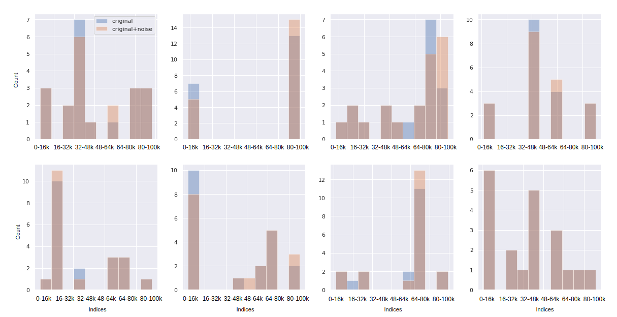
Figure 4.4: We picture the key access distribution for each head. As we see there is a little perturbation in the distribution when we apply the random region crop in the input image.

4.1.2 Experiments on ImageNet

We have conducted further experiments on the ImageNet-2012 dataset [67], assuming that the large size of the train set of the ImageNet would be more natural fit for our memory layer. The only issue was time limitations we had and the hard task of tuning the optimizer for the memory layer. Since it takes 90 epochs for the ImageNet to finish training with Resnet-50 and on NVIDIA M40 GPU it takes 14 days [85], the experiments with the size of 224$\times$224 weren’t reasonable. And since we have decided to increase the spatial size of the query input in the memory, the inference performance of the models plummeted. Therefore we have decided to resize the sizes of the images in train and validation to 64$\times$64 and run the pipeline. We kept the same augmentation pipeline as in [30].

First steps were to run the ResNet-50 augmented with the memory layer and compare it with the baseline results. The augmentation logic we have chosen for the ImageNet experiments were simpler. We have inserted the additional layer before the 44th layer of the network, where the image has the 7$\times$7 spatial size, this meant that the queries consisted of 49 feature vectors that are batched together to be fed to the memory layer. The memory size of the experiments was set to 256k, we have looked at the top-30 indices during the memory access and the batch size was set to 256. As the distance metric, we have chosen the cosine similarity with $\alpha=1$. We haven’t used dropout on the retrieved indices. SGD [65] was chosen as the optimizer with the initial learning rate of $10^{-1}$, weight decay for dense parameters of 0.0001 and momentum of 0.9. We haven’t set the weight decay for memory parameters because of the inferior results, more experiments should be conducted to find the reason for this.

The results are given in 4.2.

	accuracy, top1	utilization	FLOPs	inference, ms
ResNet-50, 64$\times$64	61.45 (61.24$\pm$0.12)	-	$\sim$338M	11ms
ResNet-50+M, 64$\times$64, skip=True,heads=8	61.61	$\sim$98%	$\sim$382M	23ms
ResNet-50+M, 64$\times$64, skip=True,heads=8, $\text{lr}_{key}$=$10^{2}$	61.82 (61.59$\pm$0.17)	$\sim$96%	$\sim$382M	23ms
ResNet-50+M, 64$\times$64, skip=True,heads=8, $\text{lr}_{key}$=$10^{3}$	60.85	$\sim$86%	$\sim$382M	23ms
ResNet-50+M, 64$\times$64, skip=False,heads=8	54.12	$\sim$15%	$\sim$382M	23ms
ResNet-50, 32$\times$32, skip=True	42.81	-	$\sim$86.1M	6ms
ResNet-50+M, 32$\times$32, skip=True,heads=8	43.49	$\sim$98%	$\sim$100M	12ms
ResNet-50+M, 32$\times$32, skip=False,heads=8	35.68	$\sim$18%	$\sim$100M	12ms

Table 4.2: The results on the Resnet-50 and Imagenet. We have tested a number of the hyper parameters to find the best train strategy for the memory models. For now we dont see the clear picture on optimization issues.

We can see from the table that there is a small increase in the validation accuracy for the models augmented with the memory layer but the large drop in the performance (inference in the table). This is not a reasonable way of incorporating the memories with the classification models and that is why we have tried to analyze how the values in the memory were used in the inference and how did they change during the training phase. We hoped to find a way of increasing the accuracy of memory augmented models by tweaking the training pipeline. For that we have logged the gradients of the keys, memory values, memory utilization and standard deviation of the keys during the training phase.

We have observed that for the activated residual connection on the memory layer, skip=True in Figure 4.5, gradients were overall higher both for memory and key values. The utilization of the skip=True was way higher reaching almost 100%, while the skip=False run plummeted to nearly 20%. What is most interesting is that the standard deviations of the keys in skip=True were not even during all training iterations. Our first assumption of the reason for this phenomena was the low learning keys for the key parameters. Further experiments are needed to tune the learning rate parameters. As a first step, we have conducted more experiments with super-convergence [71] to find the top value learning rate for key parameters in a single cycle train. We have observed that the super-convergence leaarning rate schedule reaches $10^{6}$ before the overall loss starts to increase.

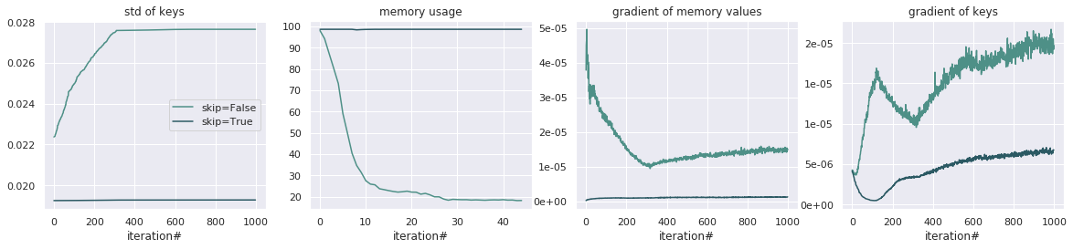
Figure 4.5: Change in values of the standard deviation of keys, memory usage, gradient of memory values, and key gradients during a training phase.

We are not aware of all the underlining issues that do not allow us to get the learning rate in a reasonable range. Maybe setting the learning rate value to $10^{6}$ is logical too, but for now, we don’t know that yet. Also, we require the augmented models to get a way better final accuracy results taking into the consideration the performance issues of the memory blocks and the amount of the additional parameters introduced into the network, i.e. $|\mathcal{M}|\cdot(d_{q}+d_{v})$ where $d_{v}$ is the dimension of values in the memory. Because of this we stop our analysis here and acknowledge the need for more experiments.

4.2 Memory in PoseNet

We have conducted some experiments on PoseNet [38] for 6-DOF camera relocalization. As it was mentioned in the previous chapter, authors of the paper have used the GoogleNet [76] the backbone for feature extraction. We have replaced it in a favour of ResNet-34 and run several models tuning the hyperparameter set, especially the scaling factor $\beta$. The Adam was the optimizer choice in these experiments. We have set the initial learning rate of $10^{-3}$ which decreases every 80 epoch. The weight decay for the dense parameters, i.e. all the parameters except the key and value vectors in the memory layer, was set to $2\times 10^{-4}$. In all the results listed, we set weight decay of memory layer to zero, Setting higher values for the weight decay was the plan of our initial experiments also, as we have hoped to provide some regularization for the values in the memory, but even the smallest weight decay failed to give us any reasonable results. We acknowledge that the additional work should be done here to find the reason behind this issue. We have set the memory size to 1k/10k and compared the results. Overall we have trained the models to the 250th epoch and have observed the plateau in the train loss.

We have initiated the experiments on the King’s College outdoor relocalization [38] which is the dataset with the images from Cambridge landmark. There are overall 1220 images in the train set and nearly 350 in the validation set. The small train set size has discouraged us to apply larger memory sizes $|\mathcal{M}|$. Since the validation set is relatively large, we have assumed that the validation accuracy could give us an overview of how good the memory layers generalize to the dataset. For the augmentation part, we have resized the images to 256$\times$256 and applied a random crop of 224$\times$224, the same set of transformations have been done in the validation. We have set the batch size of the train set to 75 and run the experiments, the results are listed in Table 4.3.

	validation	train loss	inference	FLOPs	utiliazation
$L_{r}(q_{1},q_{2})=\left\|\mathbf{q}_{1}-\mathbf{q}_{2}\right\|,q^{0}_{i}\in\mathbb{R}^{+}$
PN (PoseNet), $\beta=1$	3.02m, 3.17∘	37.5	5.6ms	$\sim$3B	-
PN, $\beta=0.1$	1.57m, 5.73∘	6.57	5.6ms	$\sim$3B	-
PN+LM, $\beta=1$	3.24m, 3.43∘	34.5	5.8ms	$\sim$(3B+10M)	-
PN+M, heads=1, $\beta=1$, $|\mathcal{M}|=1k$	3.47m, 3.49∘	10.81	6ms	$\sim$(3B+16k)	20-30%
PN+M, heads=16, $\beta=1$, $|\mathcal{M}|=1k$, dp=0.3	4.43m, 7.23∘	14.27	13ms	$\sim$(3B+16k)	95-100%
PN+M, heads=16, $\beta=1$, $|\mathcal{M}|=1k$	2.19m, 2.99∘	7.94	13ms	$\sim$(3B+16k)	95-100%
PN+M, heads=16, $\beta=0.1$, $|\mathcal{M}|=1k$	1.47m, 5.02∘	1.76	13ms	$\sim$(3B+16k)	95-100%
PN+M, heads=16, $\beta=0.1$, $|\mathcal{M}|=10k$	1.44m, 4.98∘	1.68	15ms	$\sim$(3B+50k)	50-55%
$L_{r}(q_{1},q_{2})=\min\left\{\left\|\mathbf{q}_{1}-\mathbf{q}_{2}\right\|,\left\|\mathbf{q}_{1}+\mathbf{q}_{2}\right\|\right\}$
PN (PoseNet), $\beta=1$	2.86m, 3.42∘	33.1	5.6ms	$\sim$3B	-
PN, $\beta=0.1$	1.59m, 5.36∘	6.45	5.6ms	$\sim$3B	-
PN+M, heads=16, $\beta=1$, $|\mathcal{M}|=1k$	1.87m, 2.53∘	7.41	13ms	$\sim$(3B+16k)	80-95%
PN+M, heads=16, $\beta=0.1$, $|\mathcal{M}|=1k$	1.42m, 4.38∘	1.63	13ms	$\sim$(3B+16k)	80-95%

Table 4.3: Results on the King’s College dataset, $\mathrm{trans}$ and $\mathrm{rot}$ are the translation and rotation errors respectively. We see a huge decrease in the loss on the train set for the networks with memory augmentation but also the increase in the inference time. Inference values calculated on the GTX-1080Ti with the batch size of 1.

We have compared the memory networks with the wide MLP layer that is defined as LM in the table. As in the classification experiments, the MLP layer consists of the two projection matrices and the nonlinearity between. First projections matrix maps the input vector $v_{in}\in\mathbb{R}^{d_{in}}$ to the $\mathbb{R}^{2k}$ then applying ReLU on the result we project the vector back to $\mathbb{R}^{d_{in}}$. We are using the residual on the MLP. As it can be seen from the table replacing the memory with MLP increases the train and the validation results both for rotation and positional losses. For now, we don’t understand why the replacement of the memory layer with the MLP can’t compete in the final score with the memory block augmentation.

Overall we have seen the huge decrease in the train loss for memory models, while the validation loss, though decreased both for rotation and position loss, didn’t give us as a steep decrease in the value as we have expected. We assume that the more elaborate regularization technique could be applied here. But for now we have applied the naive dropout regularization on retrieved keys which didn’t give us any promising results (dp=0.3 for dropout rate in the Table 4.3).

Though getting better numbers overall we are seeing the huge inference time increase for all the models augmented with the memory.

4.2.1 Analysis of the memory layer

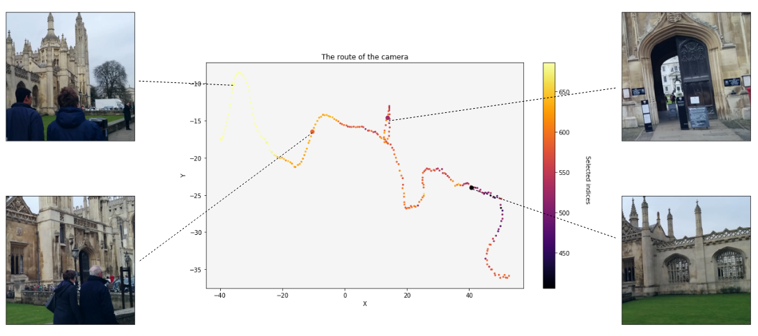
Figure 4.6: The camera path and the four sample images captures in the given coordinates. We see the correlation between the traveled distance and the indices selected.

To get a better picture of how the memory layer is utilized in regressing the position coordinates, we have plotted the distribution of the accessed keys for each image. We have scattered 200 first images in the validation set by their x,y coordinates. We have set the colour for each point ranging it from 0 to $|\mathcal{M}|$. To calculate the colour for a particular image we have gathered the key indices that were used in the forward operation, averaged and rounded to the nearest integer. The results are given in Figure 4.6.

We see that there is a correlation between the distance passed by the camera and the colours of the point, as they get darker with more distance, i.e. use lower key indices. We could assume that the memory can capture the spatial differences between the images and interpret them in the right manner.

4.3 Image reconstruction experiments

We have conducted several experiments to test the performance of the memory layers in the reconstruction tasks. For that, we have constructed a naive encoder-decoder neural network with the memory augmentation in the decoder. The overall overview of the architecture is described above.

We have experiment with the various types of memory placement: right after the latent vector (mem_idx=0), after the first layer in the decoder (mem_idx=1) and so on. We have used the Adam [42] optimizer with the initial learning rate of $10^{-3}$ and $\beta_{1}=0.9$, $\beta_{2}=0.98$. ImageNet samples were resized to 64 $\times$ 64 before training the model. We have chosen $L_{2}$ norm as the objective. Also, we used the memory size of 100k, k parameter top-k procedure of 30 and disabled dropout. The results are given in the Table 4.4.

	train loss	validation loss	inference, ms	utilization, %
Baseline	0.092	0.0076	4.3ms	-
Baseline+M, heads=1, mem_idx=0	0.0773	0.0056	4.3ms	0-10
Baseline+M, heads=4, mem_idx=0	0.075	0.0045	5ms	10-20
Baseline+M, heads=8, mem_idx=0	0.0734	0.0044	6.3ms	20-40
Baseline+M, heads=1, mem_idx=1	0.0721	0.0042	12.1ms	40-50
Baseline+M, heads=4, mem_idx=1	0.0693	0.0037	15.4ms	50-60
Baseline+M, heads=8, mem_idx=1	0.0675	0.0035	17.7ms	60-65
Baseline+M, heads=1, mem_idx=2	0.0628	0.0026	21.4ms	85-90
Baseline+M, heads=4, mem_idx=2	0.0544	0.0019	26.7ms	90-100

Table 4.4: Reconstruction results after 1600 iterations. The memory utilization numbers are approximate since the amount of experiments conducted was low. The inference speed is calculated on GTX-1080Ti with batch size of 1.

We see the steady decline in the train and validation losses with increasing the number of heads and the index of the layer of the decoder where the memory is being inserted, mem_idx. Utilization numbers increase which again supports the experiments we have conducted before. As the inference time giving us the degraded performance with mem_idx=2. This didn’t allow us to conduct more experiments with large spatial shapes of the input images. We include some reconstruction examples from the validation set in Figure 4.7.

The overall pipeline and the more details on the final architecture will be given in the released code. For now, it is important to get an understating of the overall reconstruction improvements with the memory augmentation and if it is reasonable to be used with the performance issues in mind.

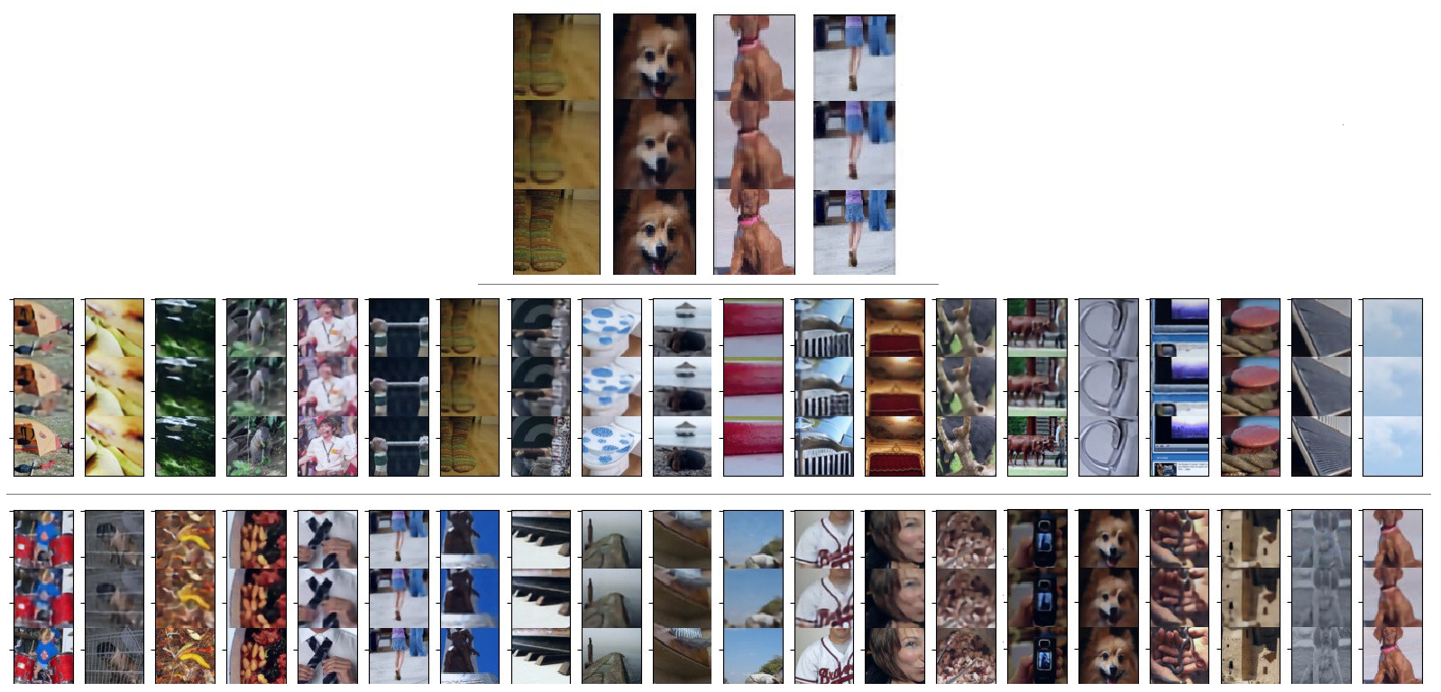
Figure 4.7: Reconstruction results. Top row images in each section are the reconstruction results with the memory augmented autoencoder with mem_idx=2 and heads=8, the middle are the output of the baseline autoencoder while the final row are the input images. We see that there are some little details that are captured using the memory layer.

4.4 Other experiments

We have also applied other experiments with memory usage in distillation [31], implicit shape modelling [10] and NERF (Representing Scenes as Neural Radiance Fields for View Synthesis) [52]. Overall, for now we can conclude that the large batch sizes of these models’ training pipelines, i.e. point coordinate samples for implicit modeling and the sampled rays for view synthesis in NERF, is the hurdle which won’t allow the memory to be used in the most efficient way, because of the difficulty of the random access parallelization with modern GPUs. Though we see some potential in knowledge distillation from very large models and more work should be conducted in this direction.

Chapter 5 Conclusion

This work analyzes the usage of product key-value memory in computer vision applications with a deep dive into the problems like image classification, regression (in the context of the camera relocalization, and the image reconstruction). We have found that for some of the problems the product key memory layer was able to provide significant speed/accuracy improvements with the high utilization of the key-value elements, while others require more careful fine-tuning and an efficient regularization strategy. We also find that the ”dying keys” affect the image classification problems. To help us tackle with it, we introduce a simple technique of memory re-initialization which helps us to eliminate ”unused” key-value pairs from the memory and cleverly re-initialize new keys that, with high probability, will be used in next iterations of training.

We show that the re-initialization has a huge impact on a toy example of randomly labelled data and observe some gains in performance on the image classification tasks.

In addition to the promising results in the experiments with the camera relocalization, we have also shown that the choice of the set of memory accessed indices in the inference depends on the spatial correlations of the input images. This signals us about the perseverance of the generalization property of the memory layer with no additional regularization required. Still, validation results didn’t meet our expectations and at this point, we could only assume that more work is required in defining more elaborate regularization strategies.

We hope that the re-initialization training strategy could be applied in large language models with exaggerated number of heads [61, 16, 9]. As we have analyzed, smaller number of heads gave a significant boost in performance.

References

- [1] Davide Abati, Jakub Tomczak, Tijmen Blankevoort, Simone Calderara, Rita Cucchiara, and Babak Ehteshami Bejnordi. Conditional channel gated networks for task-aware continual learning, 2020.
- [2] Alexandr Andoni, Piotr Indyk, Thijs Laarhoven, Ilya Razenshteyn, and Ludwig Schmidt. Practical and optimal lsh for angular distance. In C. Cortes, N. D. Lawrence, D. D. Lee, M. Sugiyama, and R. Garnett, editors, Advances in Neural Information Processing Systems 28, pages 1225–1233. Curran Associates, Inc., 2015.
- [3] Joris Baan, Maartje ter Hoeve, Marlies van der Wees, Anne Schuth, and Maarten de Rijke. Understanding multi-head attention in abstractive summarization. arXiv preprint arXiv:1911.03898, 2019.
- [4] Artem Babenko and Victor Lempitsky. The inverted multi-index. IEEE transactions on pattern analysis and machine intelligence, 37(6):1247–1260, 2014.
- [5] Dzmitry Bahdanau, Kyunghyun Cho, and Yoshua Bengio. Neural machine translation by jointly learning to align and translate. arXiv preprint arXiv:1409.0473, 2014.
- [6] Dmitry Baranchuk, Artem Babenko, and Yury Malkov. Revisiting the inverted indices for billion-scale approximate nearest neighbors. In The European Conference on Computer Vision (ECCV), September 2018.
- [7] Irwan Bello, Barret Zoph, Ashish Vaswani, Jonathon Shlens, and Quoc V. Le. Attention augmented convolutional networks. In The IEEE International Conference on Computer Vision (ICCV), October 2019.
- [8] Emmanuel Bengio, Pierre-Luc Bacon, Joelle Pineau, and Doina Precup. Conditional computation in neural networks for faster models. arXiv preprint arXiv:1511.06297, 2015.
- [9] Tom B. Brown, Benjamin Mann, Nick Ryder, Melanie Subbiah, Jared Kaplan, Prafulla Dhariwal, Arvind Neelakantan, Pranav Shyam, Girish Sastry, Amanda Askell, Sandhini Agarwal, Ariel Herbert-Voss, Gretchen Krueger, Tom Henighan, Rewon Child, Aditya Ramesh, Daniel M. Ziegler, Jeffrey Wu, Clemens Winter, Christopher Hesse, Mark Chen, Eric Sigler, Mateusz Litwin, Scott Gray, Benjamin Chess, Jack Clark, Christopher Berner, Sam McCandlish, Alec Radford, Ilya Sutskever, and Dario Amodei. Language models are few-shot learners, 2020.
- [10] Zhiqin Chen and Hao Zhang. Learning implicit fields for generative shape modeling. 2019 IEEE/CVF Conference on Computer Vision and Pattern Recognition (CVPR), Jun 2019.
- [11] Heng-Tze Cheng, Mustafa Ispir, Rohan Anil, Zakaria Haque, Lichan Hong, Vihan Jain, Xiaobing Liu, Hemal Shah, Levent Koc, Jeremiah Harmsen, and et al. Wide & deep learning for recommender systems. Proceedings of the 1st Workshop on Deep Learning for Recommender Systems - DLRS 2016, 2016.
- [12] Kyunghyun Cho and Yoshua Bengio. Exponentially increasing the capacity-to-computation ratio for conditional computation in deep learning. arXiv preprint arXiv:1406.7362, 2014.
- [13] Cesc Chunseong Park, Byeongchang Kim, and Gunhee Kim. Attend to you: Personalized image captioning with context sequence memory networks. In The IEEE Conference on Computer Vision and Pattern Recognition (CVPR), July 2017.
- [14] Jean-Baptiste Cordonnier, Andreas Loukas, and Martin Jaggi. On the relationship between self-attention and convolutional layers. In International Conference on Learning Representations, 2020.
- [15] Andrew Davis and Itamar Arel. Low-rank approximations for conditional feedforward computation in deep neural networks. 2013.
- [16] Jacob Devlin, Ming-Wei Chang, Kenton Lee, and Kristina Toutanova. Bert: Pre-training of deep bidirectional transformers for language understanding. arXiv preprint arXiv:1810.04805, 2018.
- [17] Xiaohan Ding, Xiangxin Zhou, Yuchen Guo, Jungong Han, Ji Liu, et al. Global sparse momentum sgd for pruning very deep neural networks. In Advances in Neural Information Processing Systems, pages 6379–6391, 2019.
- [18] M. Douze, H. Jegou, and C. Schmid. Product quantization for nearest neighbor search. IEEE Transactions on Pattern Analysis & Machine Intelligence, 33(01):117–128, jan 2011.
- [19] Eugene Edgington and Patrick Onghena. Randomization Tests. Statistics: A Series of Textbooks and Monographs. Addison-Wesley, Reading, Massachusetts, 2007.
- [20] Leon A Gatys, Alexander S Ecker, and Matthias Bethge. A neural algorithm of artistic style. arXiv preprint arXiv:1508.06576, 2015.
- [21] Tiezheng Ge, Kaiming He, Qifa Ke, and Jian Sun. Optimized product quantization for approximate nearest neighbor search. In The IEEE Conference on Computer Vision and Pattern Recognition (CVPR), June 2013.
- [22] Aristides Gionis, Piotr Indyk, and Rajeev Motwani. Similarity search in high dimensions via hashing. VLDB, 1999.
- [23] Ian Goodfellow, Jean Pouget-Abadie, Mehdi Mirza, Bing Xu, David Warde-Farley, Sherjil Ozair, Aaron Courville, and Yoshua Bengio. Generative adversarial nets. In Z. Ghahramani, M. Welling, C. Cortes, N. D. Lawrence, and K. Q. Weinberger, editors, Advances in Neural Information Processing Systems 27, pages 2672–2680. Curran Associates, Inc., 2014.
- [24] GFosta H. Granlund and Hans Knutsson. Signal Processing for Computer Vision. Kluwer Academic Publishers, USA, 1995.
- [25] Edouard Grave, Moustapha M Cisse, and Armand Joulin. Unbounded cache model for online language modeling with open vocabulary. In I. Guyon, U. V. Luxburg, S. Bengio, H. Wallach, R. Fergus, S. Vishwanathan, and R. Garnett, editors, Advances in Neural Information Processing Systems 30, pages 6042–6052. Curran Associates, Inc., 2017.
- [26] A. Graves, A. Mohamed, and G. Hinton. Speech recognition with deep recurrent neural networks. In 2013 IEEE International Conference on Acoustics, Speech and Signal Processing, pages 6645–6649, 2013.
- [27] Alex Graves, Greg Wayne, and Ivo Danihelka. Neural turing machines. arXiv preprint arXiv:1410.5401, 2014.
- [28] Evan Greensmith, Peter L. Bartlett, and Jonathan Baxter. Variance reduction techniques for gradient estimates in reinforcement learning. In T. G. Dietterich, S. Becker, and Z. Ghahramani, editors, Advances in Neural Information Processing Systems 14, pages 1507–1514. MIT Press, 2002.
- [29] Kaiming He, Xiangyu Zhang, Shaoqing Ren, and Jian Sun. Delving deep into rectifiers: Surpassing human-level performance on imagenet classification. In Proceedings of the IEEE international conference on computer vision, pages 1026–1034, 2015.
- [30] Kaiming He, Xiangyu Zhang, Shaoqing Ren, and Jian Sun. Deep residual learning for image recognition. In Proceedings of the IEEE conference on computer vision and pattern recognition, pages 770–778, 2016.
- [31] Geoffrey Hinton, Oriol Vinyals, and Jeff Dean. Distilling the knowledge in a neural network. arXiv preprint arXiv:1503.02531, 2015.
- [32] Jie Hu, Li Shen, and Gang Sun. Squeeze-and-excitation networks. In IEEE Conference on Computer Vision and Pattern Recognition, 2018.
- [33] Sergey Ioffe and Christian Szegedy. Batch normalization: Accelerating deep network training by reducing internal covariate shift. In Francis Bach and David Blei, editors, Proceedings of the 32nd International Conference on Machine Learning, volume 37 of Proceedings of Machine Learning Research, pages 448–456, Lille, France, 07–09 Jul 2015. PMLR.
- [34] Eric Jang, Shixiang Gu, and Ben Poole. Categorical reparameterization with gumbel-softmax. 2017.
- [35] Young Kyun Jang and Nam Ik Cho. Generalized product quantization network for semi-supervised hashing. arXiv preprint arXiv:2002.11281, 2020.
- [36] Alexander V Kashkovsky, Anton A Shershnev, and Pavel V Vashchenkov. Aspects of gpu perfomance in algorithms with random memory access. In AIP Conference Proceedings, volume 1893, page 030047. AIP Publishing LLC, 2017.
- [37] Alex Kendall and Roberto Cipolla. Geometric loss functions for camera pose regression with deep learning. In Proceedings of the IEEE Conference on Computer Vision and Pattern Recognition, pages 5974–5983, 2017.
- [38] Alex Kendall, Matthew Grimes, and Roberto Cipolla. Posenet: A convolutional network for real-time 6-dof camera relocalization. In Proceedings of the 2015 IEEE International Conference on Computer Vision (ICCV), ICCV ’15, page 2938–2946, USA, 2015. IEEE Computer Society.
- [39] Urvashi Khandelwal, Omer Levy, Dan Jurafsky, Luke Zettlemoyer, and Mike Lewis. Generalization through memorization: Nearest neighbor language models. In International Conference on Learning Representations, 2020.
- [40] Amir Hosein Khasahmadi, Kaveh Hassani, Parsa Moradi, Leo Lee, and Quaid Morris. Memory-based graph networks. In International Conference on Learning Representations, 2020.
- [41] Youngjin Kim, Minjung Kim, and Gunhee Kim. Memorization precedes generation: Learning unsupervised GANs with memory networks. In International Conference on Learning Representations, 2018.
- [42] Diederick P Kingma and Jimmy Ba. Adam: A method for stochastic optimization. In International Conference on Learning Representations (ICLR), 2015.
- [43] Alex Krizhevsky. Learning multiple layers of features from tiny images. Technical report, 2009.
- [44] Alex Krizhevsky, Ilya Sutskever, and Geoffrey E Hinton. Imagenet classification with deep convolutional neural networks. In F. Pereira, C. J. C. Burges, L. Bottou, and K. Q. Weinberger, editors, Advances in Neural Information Processing Systems 25, pages 1097–1105. Curran Associates, Inc., 2012.
- [45] Alex Krizhevsky, Ilya Sutskever, and Geoffrey E Hinton. Imagenet classification with deep convolutional neural networks. In F. Pereira, C. J. C. Burges, L. Bottou, and K. Q. Weinberger, editors, Advances in Neural Information Processing Systems 25, pages 1097–1105. Curran Associates, Inc., 2012.
- [46] Guillaume Lample, Alexandre Sablayrolles, Marc' Aurelio Ranzato, Ludovic Denoyer, and Herve Jegou. Large memory layers with product keys. In H. Wallach, H. Larochelle, A. Beygelzimer, F. d'Alché-Buc, E. Fox, and R. Garnett, editors, Advances in Neural Information Processing Systems 32, pages 8548–8559. Curran Associates, Inc., 2019.
- [47] Sangho Lee, Jinyoung Sung, Youngjae Yu, and Gunhee Kim. A memory network approach for story-based temporal summarization of 360° videos. In The IEEE Conference on Computer Vision and Pattern Recognition (CVPR), June 2018.
- [48] Christos Louizos, Max Welling, and Diederik P. Kingma. Learning sparse neural networks through regularization. In International Conference on Learning Representations, 2018.
- [49] Chris J. Maddison, Andriy Mnih, and Yee Whye Teh. The concrete distribution: A continuous relaxation of discrete random variables. 2016. cite arxiv:1611.00712.
- [50] Y. A. Malkov and D. A. Yashunin. Efficient and robust approximate nearest neighbor search using hierarchical navigable small world graphs. IEEE Transactions on Pattern Analysis and Machine Intelligence, 42(4):824–836, 2020.
- [51] Hongzi Mao, Shaileshh Bojja Venkatakrishnan, Malte Schwarzkopf, and Mohammad Alizadeh. Variance reduction for reinforcement learning in input-driven environments. In International Conference on Learning Representations, 2019.
- [52] Ben Mildenhall, Pratul P Srinivasan, Matthew Tancik, Jonathan T Barron, Ravi Ramamoorthi, and Ren Ng. Nerf: Representing scenes as neural radiance fields for view synthesis. arXiv preprint arXiv:2003.08934, 2020.
- [53] Markus Nagel, Rana Ali Amjad, Mart van Baalen, Christos Louizos, and Tijmen Blankevoort. Up or down? adaptive rounding for post-training quantization, 2020.
- [54] Behnam Neyshabur, Zhiyuan Li, Srinadh Bhojanapalli, Yann LeCun, and Nathan Srebro. Towards understanding the role of over-parametrization in generalization of neural networks. arXiv preprint arXiv:1805.12076, 2018.
- [55] Vlad Niculae, André F. T. Martins, Mathieu Blondel, and Claire Cardie. Sparsemap: Differentiable sparse structured inference, 2018.
- [56] Qingqun Ning, Jianke Zhu, Zhiyuan Zhong, Steven CH Hoi, and Chun Chen. Scalable image retrieval by sparse product quantization. IEEE Transactions on Multimedia, 19(3):586–597, 2016.
- [57] Adam Paszke, Sam Gross, Francisco Massa, Adam Lerer, James Bradbury, Gregory Chanan, Trevor Killeen, Zeming Lin, Natalia Gimelshein, Luca Antiga, Alban Desmaison, Andreas Kopf, Edward Yang, Zachary DeVito, Martin Raison, Alykhan Tejani, Sasank Chilamkurthy, Benoit Steiner, Lu Fang, Junjie Bai, and Soumith Chintala. Pytorch: An imperative style, high-performance deep learning library. In H. Wallach, H. Larochelle, A. Beygelzimer, F. d'Alché-Buc, E. Fox, and R. Garnett, editors, Advances in Neural Information Processing Systems 32, pages 8024–8035. Curran Associates, Inc., 2019.
- [58] Sergei Popov, Stanislav Morozov, and Artem Babenko. Neural oblivious decision ensembles for deep learning on tabular data. In International Conference on Learning Representations, 2020.
- [59] Alexander Pritzel, Benigno Uria, Sriram Srinivasan, Adrià Puigdomènech Badia, Oriol Vinyals, Demis Hassabis, Daan Wierstra, and Charles Blundell. Neural episodic control. In Doina Precup and Yee Whye Teh, editors, Proceedings of the 34th International Conference on Machine Learning, volume 70 of Proceedings of Machine Learning Research, pages 2827–2836, International Convention Centre, Sydney, Australia, 06–11 Aug 2017. PMLR.
- [60] Alec Radford, Luke Metz, and Soumith Chintala. Unsupervised representation learning with deep convolutional generative adversarial networks. arXiv preprint arXiv:1511.06434, 2015.
- [61] Alec Radford, Jeff Wu, Rewon Child, David Luan, Dario Amodei, and Ilya Sutskever. Language models are unsupervised multitask learners. 2019.
- [62] Prajit Ramachandran, Niki Parmar, Ashish Vaswani, Irwan Bello, Anselm Levskaya, and Jonathon Shlens. Stand-alone self-attention in vision models. arXiv preprint arXiv:1906.05909, 2019.
- [63] Ali Razavi, Aaron van den Oord, and Oriol Vinyals. Generating diverse high-fidelity images with vq-vae-2. In H. Wallach, H. Larochelle, A. Beygelzimer, F. d'Alché-Buc, E. Fox, and R. Garnett, editors, Advances in Neural Information Processing Systems 32, pages 14866–14876. Curran Associates, Inc., 2019.
- [64] Herbert E. Robbins. A stochastic approximation method. Annals of Mathematical Statistics, 22:400–407, 2007.
- [65] Herbert E. Robbins. A stochastic approximation method. Annals of Mathematical Statistics, 22:400–407, 2007.
- [66] Christian P. Robert. The metropolis-hastings algorithm. arXiv preprint arXiv:1504.01896, 2015.
- [67] Olga Russakovsky, Jia Deng, Hao Su, Jonathan Krause, Sanjeev Satheesh, Sean Ma, Zhiheng Huang, Andrej Karpathy, Aditya Khosla, Michael Bernstein, et al. Imagenet large scale visual recognition challenge. International journal of computer vision, 115(3):211–252, 2015.
- [68] Igal Sason and Sergio Verdu. -divergence inequalities. IEEE Transactions on Information Theory, 62(11):5973–6006, Nov 2016.
- [69] Noam Shazeer, Azalia Mirhoseini, Krzysztof Maziarz, Andy Davis, Quoc Le, Geoffrey Hinton, and Jeff Dean. Outrageously large neural networks: The sparsely-gated mixture-of-experts layer. 2017.
- [70] Karen Simonyan and Andrew Zisserman. Very deep convolutional networks for large-scale image recognition. arXiv preprint arXiv:1409.1556, 2014.
- [71] Leslie N. Smith and Nicholay Topin. Super-convergence: very fast training of neural networks using large learning rates. Artificial Intelligence and Machine Learning for Multi-Domain Operations Applications, May 2019.
- [72] S Spigler, M Geiger, S d’Ascoli, L Sagun, G Biroli, and M Wyart. A jamming transition from under-to over-parametrization affects generalization in deep learning. Journal of Physics A: Mathematical and Theoretical, 52(47):474001, 2019.
- [73] Sainbayar Sukhbaatar, arthur szlam, Jason Weston, and Rob Fergus. End-to-end memory networks. In C. Cortes, N. D. Lawrence, D. D. Lee, M. Sugiyama, and R. Garnett, editors, Advances in Neural Information Processing Systems 28, pages 2440–2448. Curran Associates, Inc., 2015.
- [74] Ilya Sutskever, Oriol Vinyals, and Quoc V Le. Sequence to sequence learning with neural networks. In Z. Ghahramani, M. Welling, C. Cortes, N. D. Lawrence, and K. Q. Weinberger, editors, Advances in Neural Information Processing Systems 27, pages 3104–3112. Curran Associates, Inc., 2014.
- [75] Richard S Sutton, David A. McAllester, Satinder P. Singh, and Yishay Mansour. Policy gradient methods for reinforcement learning with function approximation. In S. A. Solla, T. K. Leen, and K. Müller, editors, Advances in Neural Information Processing Systems 12, pages 1057–1063. MIT Press, 2000.
- [76] Christian Szegedy, Wei Liu, Yangqing Jia, Pierre Sermanet, Scott Reed, Dragomir Anguelov, Dumitru Erhan, Vincent Vanhoucke, and Andrew Rabinovich. Going deeper with convolutions. In Computer Vision and Pattern Recognition (CVPR), 2015.
- [77] Mingxing Tan and Quoc Le. EfficientNet: Rethinking model scaling for convolutional neural networks. In Kamalika Chaudhuri and Ruslan Salakhutdinov, editors, Proceedings of the 36th International Conference on Machine Learning, volume 97 of Proceedings of Machine Learning Research, pages 6105–6114, Long Beach, California, USA, 09–15 Jun 2019. PMLR.
- [78] Chen-Tse Tsai, Wen-tau Yih, Chris J.C. Burges, and Scott Wen-tau Yih. Web-based question answering: Revisiting askmsr. Technical Report MSR-TR-2015-20, April 2015.
- [79] Aaron van den Oord, Oriol Vinyals, and koray kavukcuoglu. Neural discrete representation learning. In I. Guyon, U. V. Luxburg, S. Bengio, H. Wallach, R. Fergus, S. Vishwanathan, and R. Garnett, editors, Advances in Neural Information Processing Systems 30, pages 6306–6315. Curran Associates, Inc., 2017.
- [80] Ashish Vaswani, Noam Shazeer, Niki Parmar, Jakob Uszkoreit, Llion Jones, Aidan N Gomez, Ł ukasz Kaiser, and Illia Polosukhin. Attention is all you need. In I. Guyon, U. V. Luxburg, S. Bengio, H. Wallach, R. Fergus, S. Vishwanathan, and R. Garnett, editors, Advances in Neural Information Processing Systems 30, pages 5998–6008. Curran Associates, Inc., 2017.
- [81] Elena Voita, David Talbot, Fedor Moiseev, Rico Sennrich, and Ivan Titov. Analyzing multi-head self-attention: Specialized heads do the heavy lifting, the rest can be pruned. Proceedings of the 57th Annual Meeting of the Association for Computational Linguistics, 2019.
- [82] Xin Wang, Fisher Yu, Zi-Yi Dou, Trevor Darrell, and Joseph E. Gonzalez. Skipnet: Learning dynamic routing in convolutional networks. Lecture Notes in Computer Science, page 420–436, 2018.
- [83] Ran Yi, Zipeng Ye, Juyong Zhang, Hujun Bao, and Yong-Jin Liu. Audio-driven talking face video generation with learning-based personalized head pose. arXiv preprint arXiv:2002.10137, 2020.
- [84] Seungjoo Yoo, Hyojin Bahng, Sunghyo Chung, Junsoo Lee, Jaehyuk Chang, and Jaegul Choo. Coloring with limited data: Few-shot colorization via memory augmented networks. In The IEEE Conference on Computer Vision and Pattern Recognition (CVPR), June 2019.
- [85] Yang You, Zhao Zhang, James Demmel, Kurt Keutzer, and Cho-Jui Hsieh. Imagenet training in 24 minutes. arXiv preprint arXiv:1709.05011, 2017.
- [86] Chulhee Yun, Suvrit Sra, and Ali Jadbabaie. Small relu networks are powerful memorizers: a tight analysis of memorization capacity. In H. Wallach, H. Larochelle, A. Beygelzimer, F. d'Alché-Buc, E. Fox, and R. Garnett, editors, Advances in Neural Information Processing Systems 32, pages 15558–15569. Curran Associates, Inc., 2019.
- [87] Matthew D. Zeiler and Rob Fergus. Visualizing and understanding convolutional networks. Lecture Notes in Computer Science, page 818–833, 2014.
- [88] Chiyuan Zhang, Samy Bengio, Moritz Hardt, Benjamin Recht, and Oriol Vinyals. Understanding deep learning requires rethinking generalization. arXiv preprint arXiv:1611.03530, 2016.
- [89] Łukasz Kaiser, Ofir Nachum, Aurko Roy, and Samy Bengio. Learning to remember rare events. arXiv preprint arXiv:1703.03129, 2017.