Connecting the formation of stars and planets.
I – Spectroscopic characterization of host stars with TIGRE

Abstract

In search for a connection between the formation of stars and the formation of planets, a new semi-automatic spectral analysis method using iSpec was developed for the TIGRE telescope installed in Guanajuato, Mexico. TIGRE is a 1.2m robotic telescope, equipped with an Echelle spectrograph (HEROS), with a resolution R $\simeq 20000$. iSpec is a synthetic spectral fitting program for stars that allows to determine in an homogeneous way their fundamental parameters: effective temperature, $T_{\rm eff}$, surface gravity, $\log g$, metallicities, $[M/H]$ and $[Fe/H]$, and rotational velocity, $V\sin i$. In this first article we test our method by analysing the spectra of 46 stars, host of exoplanets, obtained with the TIGRE.

En la búsqueda de una conexión entre la formación estelar y planetaria, se desarrolló un nuevo método semiautomático de análisis espectral estelar usando iSpec, para el telescopio TIGRE, instalado en Guanajuato, México. El TIGRE es un telescopio robótico de 1.2m, el cuál está equipado con el espectrógrafo Echelle HEROS, que tiene una resolución R $\sim 20,000$. iSpec es un programa de ajuste espectral sintético para estrellas que permite determinar de manera homogénea sus parámetros fundamentales: temperatura efectiva, $T_{\rm eff}$, gravedad superficial, $\log g$, metalicidades, $[M/H]$ y $[Fe/H]$, y velocidad de rotación, $V\sin i$. En este artículo, probamos nuestro método, analizando una muestra de 46 estrellas observadas por el TIGRE que albergan exoplanetas.

stars: fundamental parameters stars: rotation stars: formation stars: planetary systems

0.1 Introduction

Since the discovery of the first planet orbiting another star in the 1990s, the number of confirmed exoplanets had steadily increased reaching in November of last year 4133. The urgent tasks with which we are faced now are determining the compositions of these exoplanets and understanding how they formed. However, although that should have been straightforward (Seager, 2010), the detection of new types of planets had complicated the matter, changing in a crucial way our understanding of the formation of planetary systems around stars like the Sun.

The first new type of planets to be discovered was the “hot Jupiters” (HJs; Mayor & Queloz, 1995), which are gas giants like Jupiter and Saturn, but with extremely small periods, $P<10$ days, consistent with semi-major axes smaller than $a_{p}=0.05$ AU. The existence of HJs is problematic because according to the model of formation of the solar system they can only form in the protoplanetary disk (PPD) where it is cold enough for volatile compounds such as water, ammonia, methane, carbon dioxide and monoxide to condense into solid ice grains (Plummer et al., 2005). In the solar system, this happens beyond the ice-line, which is located close to 3 AU (Martin & Livio, 2012). This implies that HJs must have formed farther out in the cold regions of the PPD, then migrated close to their stars (Lin et al., 1996). Subsequent discoveries have then shown that far from being exceptional, artifacts of an observational bias, HJs turned out to be very common around Sun-like stars, suggesting that large scale migration is a standard feature of the planet formation process (Butler et al., 2000; Udry & Santos, 2007).

Two other new types of planets discovered are the “Super-Earths” (Leconte et al., 2009; Valencia et al., 2006; Martin & Livio, 2015; Chabrier et al., 2009) and the “mini-Neptunes” (Gandolfi et al., 2017). These too were found to be common and very close to their stars, which, consequently, also makes them “hot”. Their discoveries are important for two reasons. The first reason is that it makes the alternative “in situ” model for the formation of HJs (e.g., Boss, 1997) a special model, since it cannot explain the large mass range and diversity of the “hot” exoplanets observed (Super-Earths and mini-Neptunes in situ models are discussed in Raymond et al., 2008; Chiang & Laughlin, 2013). The second reason is that it was recently established by Lee et al. (2017) that their numbers around their host stars fall rapidly for periods $P<10$ days ($\sim 0.09$ AU), which, assuming Keplerian orbits, clearly implies they all formed farther out (beyond 0.1 AU) and have migrated inward, but with a good many disappearing into their stars. This, once again, put large scale migration at the front scene of the planet formation process.

This brings us to the present fundamental question in planet formation theory (Anand et al., 2004): what explains the fact that large scale migration did not happen in the solar system? Or, in other words, assuming all planets form in a PPD around a low mass star (Nomura et al., 2016; van der Marel et al., 2018; Pérez et al., 2019), what difference would make migration more important in one case and less important in another (see discussion in Walsh et al., 2011)?

Integrating the migration process into a consistent model of planets formation is an extremely active and fast evolving field of research (a recent review of this important subject can be find in Raymond & Morbidelli, 2020). In the cases of the HJs, two migration mechanisms are accepted now as most probable (Dawson & Johnson, 2018): (1) disk migration, where the planet forms beyond the ice-line then migrates inward by loosing its orbit angular momentum to the PPD (see thorough reviews in Baruteau et al., 2014; Armitage, 2020), and (2) high-eccentricity migration, according to which the planet first gains a high eccentricity through interactions with other planets, which makes it to pass very close to its star where it looses its orbit angular momentum by tidal interactions (this is a more complicated process, involving different mechanisms; e.g., Rasio & Ford, 1996; Weidenschilling & Marzari, 1996; Marzari & Weidenschilling, 2002; Chatterjee et al., 2008; Nagasawa et al., 2008; Beaugé & Nesvorný, 2012). However, what is not clear in these two models is what importance must be put on the characteristics of the PPD, its mass, size, depth and composition?

According to PPD formation theory, there are two possible mass scenarios (Armitage, 2020): the minimum mass model, between 0.01 to 0.02 M_⊙, which suggests that the PPD initial mass is only sufficient to explain the masses of the planets that formed within it, and the maximum mass model, which suggests the mass could have been much higher, close to 0.5 M_⊙. Consequently, more massive PPD (compared to the Solar system) might have either favored the formation of more massive planets (consistent with PPD observations, see Fig. 2 and discussion in Raymond & Morbidelli, 2020) or a higher number of planets. The problem is that this makes both migration mechanisms equally probable (also, the masses observed seem too low; also related to Fig. 2 in Raymond & Morbidelli, 2020). Another caveat is that the solar system is a multiple planet system where migration on large scale did not happen.

In terms of angular momentum, the differences between the minimum and maximum mass model for the PPD might also be important. By definition, the angular momentum of a planet is given by the relation (e.g., Berget & Durrance, 2010):

$$J_{p}={M_{p}}\sqrt{GM_{*}a_{p}(1-e^{2}_{p})}$$ (1)

where $M_{p}$ and $M_{*}$ are the masses of the planet and its host star, $a_{p}$ is the semi-major axis of the planet and $e_{p}$ its eccentricity. This suggests that within the maximum mass model more massive planets would also be expected to have higher orbital angular momentum (through their PPD) and, consequently, to have lost a larger amount of their angular momentum during large scale migration ($a_{p}\rightarrow 0$). This implies that the efficiency of the migration mechanism must increase with the mass of the planet (or its PPD). In principle, such requirement might be one way to distinguish which migration process is more realistic. However, the problem is bounded to be more complicated. First, stars rotate much more slowly than expected assuming conservation of angular momentum during their formation (McKee & Ostriker, 2007). Second, defining the angular momentum of a planetary system as $J_{sys}=J_{*}+\Sigma J_{p}$ where $\Sigma J_{p}$ is the sum of the angular momentum of all the planets and $J_{*}$ the angular momentum of the host star (cf. Berget & Durrance, 2010), the angular momentum of massive planets (even after migration, assuming $a_{p}\neq 0$) will always dominate over the angular momentum of its host stars. That is, $J_{*}/\Sigma J_{p}<1$, and this is despite the enormous lost of angular momentum of the star during its formation. This implies that a sort of coupling must exist between the angular momentum of the stars and their planets through their PPDs. Understanding the nature of this coupling, therefore, is an important step in understanding how the PPD and the planets forming in it are connected to the formation of their stars. This, on the other hand, requires completing our information about the stars and the planets rotating around them.

In the case of the planets, the two most successful detection techniques, the radial velocity (RV) and transit (Tr) methods, yield estimates of the mass of a planet, $M_{p}$, and its radius, $R_{p}$, as well as the semi-major axis, $a_{p}$, and the eccentricity of its orbit, $e_{p}$. The first two parameters constrain their composition and formation process in the PPD, while the last two give information about their migration. By combining the four parameters we can also retrieve the angular momentum of the orbits of the planets (cf. Eq. 1). In the case of the stars the most important characteristics that can be derived from their spectra are the effective temperature, $T_{eff}$, the surface gravity, $\log g$, the metallicities, [M/H] or [Fe/H], and the rotational velocity, $V\sin i$. The first two can be used in combination with their magnitudes and distances (using GAIA parallaxes) to determine their radii and masses, which taken in combination with the rotational velocity yield the angular momentum (or spin) of the star, $J_{*}$:

$$J_{*}=\gamma_{*}M_{*}R_{*}V^{rot}_{*}$$ (2)

where $M_{*}$, $R_{*}$ and $\gamma_{*}$ are the star mass, radius and moment of inertia (which depends on the mass of the star; cf. Irwin, 2015), and $V^{rot}_{*}=V\sin i/\sin i$ is the equatorial rotation velocity (where $i$ is the inclination angle of the rotation axis relative to our line of sight).

To understand how the formation of planets is connected with the formation of their host stars, we must, consequently, make an effort in determining in parallel with the discovery of the former the physical characteristics of the latter. Present data banks for exoplanets (e.g., Kepler and now TESS, with 51 confirmed discoveries, and future survey like PLATO) require a lot of follow up observations and analysis for the host stars, which are usually done using large diameter telescopes equipped with high resolution spectrographs. However, for the brightest stars (TESS targets, for example, being 30-100 times brighter than KEPLER stars), the use of smaller diameter telescopes equipped with lower resolution spectrographs might be more efficient in acquiring the information. Moreover, although high resolution spectra is justified when one uses the standard spectral analysis method, which is based on modeling the equivalent width (EW) of spectral lines, this might not be necessary when one uses the synthetic spectral analysis (e.g., Valenti & Fischer, 2005), which consists in fitting observed spectra to grids of synthetic spectra with well determined physical characteristics that can be produced at different spectral resolutions. Another problem in using large aperture telescopes for host stars follow up is that since these telescopes are in high demand (for faint objects), data are collected on short duration runs by different groups using (although the same analysis method) different techniques and codes, which introduce discrepancies between the results (Hinkel et al., 2014, 2016; Blanco-Cuaresma, 2014; Jófre et al., 2017). This suggests that a follow up using a dedicated telescope and applying only one method of analysis could produce more homegeneous data (one effort to homogenize data is the Stars With ExoplanETs CATalog or SWEET-Cat for short; Sousa et al., 2008). For these reasons we developed a new method based on stellar spectral analysis for data obtained with the TIGRE telescope (Telescopio Internacional de Guanajuato Robótico Espectroscópico) that is installed at our institution in Guanajuato.

TIGRE is a 1.2 m fully robotic telescope located at the La Luz Observatory (in central Mexico) at an altitude of 2,400 m; a more detailed description can be found in Schmitt et al. (2014). Its principal instrument is the fibre-fed echelle spectrograph HEROS (Heidelberg Extended Range Optical Spectrograph), which yields a spectral resolution $R\sim 20,000$, covering a spectral range from 3800 Å  to 8800 Å. The queue observing mode and automatic reduction pipeline already implemented for this telescope allow to optimized the observation and reduction process, producing high homogeneous data rapidly and confidently. To optimize the analysis process, we have developed a semi-automatic method that allows us to derive efficiently the most important physical characteristics of the stars: $T_{eff}$, $\log g$, [M/H], [Fe/H], and $V\sin i$. This was done by applying the synthetic spectral fitting technique as offered by the code iSpec (Blanco-Cuaresma, 2014), which was shown to yield results that are comparable to results in the literature that were obtained through different methods and codes (Blanco-Cuaresma, 2019).

The goal of this first article is to explain our spectral analysis method based on iSpec and compare results obtained by TIGRE with data taken from the literature. In an accompanying paper (Flor-Torres et al., hereafter paper II) we will present a preliminary study, based on our own observational results, about the coupling of the angular momentum of the exoplanets and their host stars.

0.2 Sample of host stars with exoplanets observed with TIGRE

Our initial target list for a pilot project was built from the revised compendium of confirmed exoplanets in the Exoplanet Orbit Database (hereafter Exoplanets.org, selecting all the stars with spectral type F, G or K, located on the main sequence (based on their luminosities and colors), and for which a confirmed planet with well determined mass, radius, and semi-major axis was reported. Note that we did not apply a restriction to single systems, since from the point of view of the angular momentum we verified that only the major planet of a system counts (like Jupiter in our solar system). To optimize our observation with TIGRE, we restricted further our target list by retaining only host stars that have a magnitude V $\leq 10.5$, obtaining a much shorter list of 65 targets.

Our observed sample consists of 46 stars, host of 59 exoplanets, which were observed by TIGRE in queue mode. In Table 1 the stars observed are given a running number (col. 1) which is used to identified them in the different graphics. The magnitude in V of each star and its distance as calculated from Gaia parallaxes are given in col. 3 and 4 respectively. Also shown are the exposure time, in col. 5, and signal to noise (S/N) in col. 6, as measured in the red part of the spectrum. The last column gives the main references found in the literature with data about the host stars and their planetary systems.

The HEROS spectrograph on TIGRE is coupled to two ANDOR CCDs, cooled by thermocouple (Peltier cooling to -100 C): blue iKon-L camera DZ936N-BBB and red iKon-L camera DZ936N-BV. This yields for each star two spectra, one in the blue, covering a spectral range from 3800 Å  to 5750 Å, and one in the red, covering a spectral range from 5850 Å to 8750 Å. All the data were automatically reduced by the TIGRE/HEROS standard pipeline, which applies automatically all the necessary steps to extract Echelle spectra (Hempelmann et al., 2016; Mittag et al., 2016): bias subtraction, flat fielding, cosmic ray correction, order definition and extraction and wavelength calibration, which was carried out by means of Th-Ar lamp spectra taken at the beginning and end of each night. Finally, we applied a barycentric correction and as a final reduction step, corrected each spectrum for telluric lines using the code Molecfit developed by Smette et al. (2015). After verification of the results of the reduction process, we decided to concentrate our spectral analysis only on the red part of the spectra where the S/N is higher.

Table 1: Stars observed with the TIGRE

Id. #	Star	Magnitude	Distance	Exp. time	S/N	Ref.
		(V)	(pc)	(min)		(as found in exoplanets.org)
1	*KELT-6	10.3	242.4	97.1	54	Damasso et al. (2015)
2	*HD 219134	5.6	6.5	8.0	139	Motalebi et al. (2015)
3	*KEPLER-37	9.8	64.0	93.2	75	Batalha et al. (2013)
4	HD 46375	7.8	29.6	108.0	107	Marcy et al. (2000)
5	HD 75289	6.4	29.1	37.8	99	Udry et al. (2000)
6	HD 88133	8.0	73.8	116.0	94	Fischer et al. (2005)
7	HD 149143	7.9	73.4	108.0	93	Fischer et al. (2006); da Silva et al. (2006)
8	HAT-P-30	10.4	215.3	100.9	59	Johnson et al. (2011)
9	KELT-3	9.8	211.3	92.5	68	Pepper et al. (2013)
10	KEPLER-21	8.3	108.9	29.4	83	Borucki et al. (2011)
11	KELT-2A	8.7	134.6	54.3	95	Beatty et al. (2012)
12	HD86081	8.7	104.2	61.4	100	Johnson et al. (2006)
13	WASP-74	9.8	149.8	96.5	73	Hellier et al. (2015)
14	HD 149026	8.1	76.0	37.4	98	Sato et al. (2005)
15	HD 209458	7.6	48.4	40.0	98	Henry et al. (2000); Charbonneau et al. (2000)
16	BD-10 3166	10.0	84.6	100.8	72	Butler et al. (2000)
17	HD 189733	7.6	19.8	33.1	102	Bouchy et al. (2005)
18	HD 97658	7.7	21.6	35.0	123	Howard et al. (2011)
19	HAT-P-7	10.5	344.5	43.5	32	Pál et al. (2008)
20	KELT-7	8.5	137.2	47.2	93	Bieryla et al. (2015)
21	HAT-P-14	10.0	224.1	84.0	57	Torres et al. (2010)
22	WASP-14	9.7	162.8	74.6	66	Joshi et al. (2009)
23	HAT-P-2	8.7	128.2	70.0	69	Bakos et al. (2007)
24	WASP-38	9.4	136.8	75.8	82	Barros et al. (2011)
25	HD 118203	8.1	92.5	41.5	92	da Silva et al. (2006)
26	HD 2638	9.4	55.0	104.6	82	Moutou et al. (2005)
27	WASP-13	10.4	229.0	123.7	51	Skillen et al. (2009)
28	WASP-34	10.3	132.6	136.8	62	Smalley et al. (2011)
29	WASP-82	10.1	277.8	98.1	51	West et al. (2016)
30	HD17156	8.2	78.3	46.3	98	Fischer et al. (2007)
31	XO-3	9.9	214.3	70.8	60	Johns-Krull et al. (2008)
32	HD 33283	8.0	90.1	53.4	101	Johnson et al. (2006)
33	HD 217014	5.5	15.5	40.0	254	Mayor & Queloz (1995)
34	HD 115383	5.2	17.5	4.0	105	Kuzuhara et al. (2013)
35	HAT-P-6	10.5	277.5	125.0	49	Noyes et al. (2008)
36	*HD 75732	6.0	12.6	28.7	141	Marcy et al. (2002)
37	HD 120136	4.5	15.7	9.3	174	Butler et al. (2000)
38	WASP-76	9.5	195.3	91.1	73	West et al. (2016)
39	Hn-Peg	6.0	18.1	8.0	99	Luhman et al. (2007)
40	WASP-8	9.9	90.2	150.0	81	Queloz et al. (2010)
41	WASP-69	9.9	50.0	90.0	76	Anderson et al. (2014)
42	HAT-P-34	10.4	251.1	105.0	56	Bakos et al. (2012)
43	HAT-P-1	9.9	159.7	75.0	60	Bakos et al. (2007)
44	WASP-94 A	10.1	212.5	105.0	58	Neveu-VanMalle et al. (2014)
45	WASP-111	10.3	300.5	90.0	58	Anderson et al. (2014)
46	HAT-P-8	10.4	212.8	150.0	74	Latham et al. (2009)
An * in front of the name of the star identified multiple planetary systems.

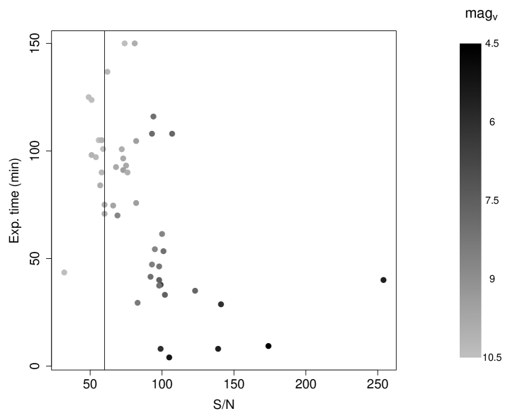
Figure 1: S/N as a function of exposure time for our sample, limited to stars with magnitude limit V $\leq 10.5$. Note that the exposure time was adjusted to reach S/N $\geq\leavevmode\nobreak\ 60$ in less than two hours.

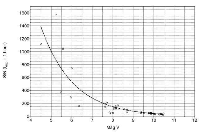
Figure 2: Exponential growth curve giving the S/N expected after one hour exposure time for stars with different magnitudes.

In Fig. 1 we traced the S/N obtained as a function of the exposure time. For each star the total exposure time during observation was adjusted to reach S/N $\geq 60$. Note that this result only depends on the telescope diameter, the fiber transmission, the spectrograph resolution (we used R = 20,000, but the resolution is adjustable in iSpec) and the photometric conditions (explaining most of the variance).The average exposure time was 74 s for an average S/N $\sim 87$, which makes observation with TIGRE a very efficient process.

To determine how faint a follow up with TIGRE could be done efficiently, we traced in Fig. 2 an exponential growth curve based on our data, determining the S/N expected in one hour for stars with different magnitudes. One can see that a star with 10.5 mag in V would be expected to have a S/N near 30 (or 60 in 2 hours). The lower we could go would be S/N $\sim 10$ which would be reached in one hour by a 12.5 mag star (or 2 hours for 13 mag star). Since it is not clear how low the S/N of a star could be to be efficiently analysed using the synthetic-spectra method, we judged safer to adopt a limit S/N of 60, which can be reach within two hours using TIGRE. This justify the magnitude limit, V $\leq 10.5$, adopted for this pilot project. Our observations suggest that a 1.2 m telescope could contribute significantly to follow up of exoplanet surveys like TESS, searching for small rocky planets around bright stars (stars much brighter than KEPLER stars), and in the near future PLATO, which will search for Earth-like planets in the habitable zones of one million nearby Solar type stars.

0.3 Spectral analysis using iSpec

Our spectral analysis was developed using the synthetic spectral fitting technique offered by the code iSpec (version 2016.11.18; Blanco-Cuaresma, 2014, 2019). In brief, this technique consists in comparing an observed spectrum with synthetic spectra interpolated from pre-computed grids, calculated using different radiative transfer codes, and applying a least-square minimization algorithm to converge towards the closest approximation possible. In Fig. 3 we show one example of a synthetic spectral fit for the star HD 46375. The fit has a rms 0.0319, which is relatively good considering HEROS intermediate resolution (Piskunov & Valenti, 2017). Due to the low resolution of our spectra we can fit at the same time in an homogeneous manner the intensity and spectral profiles of more than 100 lines (compared to a few 10s at high resolution; e.g., Valenti & Fischer, 2005). The best fit then allows to determine five important atmospheric parameters: i.e., the effective temperature, $T_{eff}$, the surface gravity, $\log g$, two indexes of metallicities, $[M/H]$ and $[Fe/H]$, and the rotational velocity, $V\sin i$.

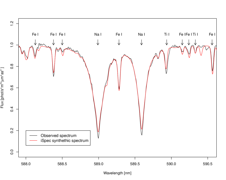
Figure 3: Example of the result for the synthetic spectral fitting method in iSpec. The star is HD 46375, the observed spectrum is in blue and the fitted spectrum in red, with a rms of 0.0319.

To optimize our analysis a crucial step of our method consisted in applying iSpec to a TIGRE spectrum from the Sun (as reflected by the Moon). Our main goal was to determine a subset of spectral lines and segments that best reproduces the physical characteristics of our star. Although this step is time consuming, because each line and segment have to be tested incrementally by running iSpec, once these lines and segments are established, the analysis of stars becomes straightforward and efficient, the full process taking only a few minutes to converge on a modern desktop computer. Starting with the whole line-list available in the VALD database (Kupka et al., 1999, 2011), we kept only 122 lines in the red for which we defined specific segments in Table LABEL:tab:B1 in the appendix 0.6. As we already verified in Eisner et al. (2020), these lines and segments can also be used in iSpec as a standard basis for observations obtained with different telescopes and (once adjusted for the resolution) other spectrographs.

Our initial analysis of the Sun also allowed us to decide which solar abundance, atmospheric model and radiative transfer code were optimal. We adopted the solar abundance of Asplund et al. (2009), the ATLAS atmospheric model of Kurucz (2005) and the radiative transfer code SPECTRUM of Gray & Corbally (1994). Another parameter that turned out to be important using iSpec is a correction for limb darkening, which we fixed to a value of 0.6 (Hestroffer & Magnan, 1998; Blanco-Cuaresma, 2019).

After working out the analysis of the Sun, we found an unexpected difficulty in obtaining the rotation velocity, $V\sin i$, for our stars. The problem comes from the fact that in low mass stars the turbulence velocity $V_{mic}$ and $V_{mac}$ have values comparable to $V\sin i$ (Doyle et al., 2014), and there is consequently no fail-proof recipe how to “constrain” these velocities using the synthetic method. One way to approach this problem (following different researchers in the field) is in adopting ad hoc values based on theory or observation (Gray, 1984a, b; Fischer & Valenti, 2005; Bruntt et al., 2010; Tsantaki et al., 2014; Doyle et al., 2014). For our analysis, we decided to adopt empirical values. For $V_{mac}$ we used the relation (Doyle et al., 2014):

$$V_{mac}=a+b\Delta T+c\Delta T^{2}-2.00(\log g-4.44)$$ (3)

where $\Delta T=(T_{eff}-5777)$, $a=3.21$, $b=2.33\times 10^{-3}$ and $c=2.00\times 10^{-6}$. For $V_{mic}$ we used the relation (Tsantaki et al., 2014):

$$V_{mic}=6.932\times 10^{-4}T_{eff}-0.348\log g-1.437$$ (4)

Note that neither authors give uncertainties on these values. However, Doyle et al. (2014) suggested generic uncertainties of the order of $\pm\ 0.27$ km/s and $\pm\ 0.15$ for $V_{mac}$ and $V_{mic}$ respectively, which we adopted for our study.

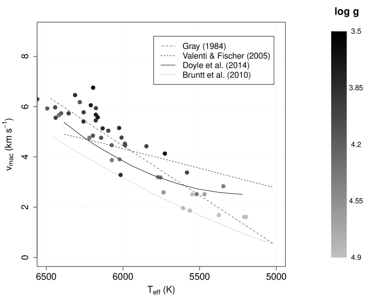
Figure 4: Values of $V_{mac}$ adopted for our analysis with iSpec as function of our results for $T_{eff}$.

In Fig. 4 we show the final values of $V_{mac}$ obtained in our analysis. Traced over the data, we draw the different relations proposed in the literature to fix this parameter. At high temperatures ($T_{eff}>5800$ K), one can see that our values for $V_{mac}$ are well above the upper limit determined by (Valenti & Fischer, 2005), while at low temperatures, the values are well above the lower limit determined by (Bruntt et al., 2010). In general, our results for $V_{mac}$ are consistent with the values expected based on the relation proposed by (Gray, 1984b).

Our final result for the Sun is shown in Table 2. These values were obtained after only ten iterations, using the parameters of the Sun as initial guess and fixing $V_{mac}$ and $V_{mic}$ using Eq. 3 and Eq. 4. For comparison sake, we also included in Table 2 the values adopted for the Gaia Benchmark stars. Although our best fit reproduces well the physical characteristics of the Sun, the uncertainty estimated by iSpec for $V\sin i$ is relatively high. But this, as we already explained, is expected considering the problem related to $V_{mic}$ and $V_{mac}$. The different solutions (as shown in Fig. 4) in solving this problem might explain, for example, why the macro turbulence we used for the Sun is lower than what was used by Gaia. In Doyle et al. (2014), the authors already noted a similar difference, by comparing the values they obtained by their relation with results reported by Fischer & Valenti (2005), where $V_{mac}$ were systematically higher by as much as $0.54\ {\rm km\ s^{-1}}$. However, adding this difference (as a systematic correction) to make our result for $V_{mac}$ closer to the value proposed in the Gaia Benchmark, did not lower the uncertainties on $V\sin i$ obtained with iSpec. Therefore, considering that our method easily reproduce the value of $V\sin i$ for the Sun, we judged more realistic to keep a high uncertainty on this parameter. Besides, the question is possibly more complex, considering the uncertainty on the existence of a $J-M$ relation, $J_{*}\propto M^{\alpha}$, for low mass stars (Herbst et al., 2007) and taking into account that $V\sin i$ might also depend on the age of the star (that is, decreasing with the age; Kraft, 1967; Wilson, 1963; Skumanich, 1972).

Table 2: Results for the Solar spectrum using iSpec

Char.	iSpec	Sun*
$T_{eff}$	$5571\pm 30$ K	$5571$ K
$\log g$	$4.44\pm 0.04$ dex	$4.44$ dex
$[M/H]$	$0.00\pm 0.03$	$0$
$[Fe/H]$	$0.00\pm 0.03$	$0$
$V\sin i$	$1.60\pm 1.45$ km/s	$1.60$ km/s
$V_{mic}$	$1.02$ km/s	$1.07$ km/s
$V_{mac}$	$3.19$ km/s	$4.21$ km/s
rms of fit	$0.0289$
*Gaia benchmark Stars values(Blanco-Cuaresma, 2019)

For the analysis of the stars, our semi-automatic method can be resumed in the following way. We first run iSpec using the parameters of the Sun as initial input. This implies calculating $V_{mac}$ and $V_{mic}$ using Eq. 3 and Eq. 4, keeping these values fixed and leaving all the other parameters free. The results of the first run give us new values of $T_{eff}$ and $\log g$ based on which we calculate new initial values for $V_{mac}$ and $V_{mic}$ before running iSpec a second time.

To verify our solutions, for each star we use the final value of $T_{eff}$ to calculate its mass and radius (first we get the mass, then the corresponding radius) using the mass-luminosity relation for stars with masses between 0.43 $M_{\odot}$ and 2 $M_{\odot}$ (Wang & Zhong, 2018):

$$\frac{M}{M_{\odot}}=(\frac{L}{L_{\odot}})^{1/4}=\frac{T_{eff}}{T_{\odot}}(\frac{R}{R_{\odot}})^{1/2}$$ (5)

where $L$ is the bolometric luminosity as determined from its magnitude in V and distance calculated from Gaia in Table 1. Then, we verified that the value of $\log g$ given by iSpec is consistent with the mass and radius obtained using the relation (Eq. 7 in Valenti & Fischer, 2005):

$$\log(M/M_{\odot})=\log(g_{*})+2\log(R/R_{\odot})-4.437$$ (6)

In general, we obtained consistent values for $\log g$, within the generic errors suggested by Doyle et al. (2014). However, for height stars, we found discrepant masses, the masses obtained using Eq. 6 being higher than the masses using Eq. 5. To solve this problem we found important to better constrain the initial value of $\log g$ before running iSpec a second time. The reason for this constrain is physically clear, since, as shown by Eq. 5 and Eq. 6, $\log g$ is coupled to $T_{eff}$. In Valenti & Fischer (2005), for example, the authors took into account this coupling by first fixing the initial value of $T_{eff}$ related to the B-V color of the star, then used a generic $\log g$ consistent with this temperature. In our case we decided to use as initial parameters for the second run the value of $T_{eff}$ obtained from the first run with iSpec (which use the values of the Sun as first guesses) and to use as second guess the value of $\log g$ given by Eq. 6 that makes the two masses consistent. This also implies recalculating $V_{mac}$ and $V_{mic}$ for this new values, which, as before, are kept fix running iSpec. The unique consequence of adding this constrain for the height stars with discrepant masses was to lower the final values of their $\log(g)$, all the other parameters being equal. For each star, our method requires only two runs of ten iterations each, which amounts to about 30 minutes CPU time on a fast desktop computer. This makes our analysis process quite efficient.

0.4 Results: characterization of the host stars of exoplanets observed with TIGRE

Table 3: Physical parameters of the host stars of exoplanets in our sample, as determined with iSpec.

No.	Name of star	$T_{eff}$	$\Delta{\rm T_{eff}}$	$logg$	$\Delta{\log g}$	[M/H]	$\Delta{[M/H]}$	$[Fe/H]$	$\Delta{[Fe/H]}$	$V\sin i$	$\Delta{V\sin i}$	$V_{mic}$	$V_{mac}$	rms	R∗	$\Delta{\rm R_{*}}$	M∗	$\Delta{\rm M_{*}}$
		(K)	(K)							(km/s)	(km/s)	(km/s)	(km/s)		($R_{\odot}$)	($R_{\odot}$)	($M_{\odot}$)	($M_{\odot}$)
1	KELT-6	6176	24	4.03	0.05	$-0.38$	0.02	$-0.14$	0.03	6.52	0.82	1.44	5.28	0.0292	1.71	0.20	1.22	0.20
2	HD 219134	5209	13	4.90	0.00	0.00	0.02	0.02	0.01	7.09	0.30	0.47	1.61	0.0318	0.54	0.09	0.77	0.09
3	KEPLER-37	5520	19	4.50	0.04	$-0.40$	0.02	$-0.28$	0.02	6.62	0.50	0.82	2.62	0.0317	0.71	0.15	0.88	0.15
4	HD 46375	5345	22	4.47	0.04	$-0.05$	0.01	0.11	0.01	2.01	0.73	0.71	2.52	0.0319	0.83	0.01	0.88	0.02
5	HD 75289	6196	23	4.16	0.06	0.16	0.02	0.42	0.02	4.11	0.56	1.41	5.10	0.0291	1.27	0.01	1.14	0.03
6	HD 88133	5582	16	4.05	0.03	0.15	0.01	0.34	0.01	1.98	0.76	1.02	3.61	0.0344	1.80	0.01	1.12	0.02
7	HD 149143	6067	20	4.36	0.04	0.17	0.02	0.48	0.02	3.53	0.61	1.25	4.22	0.0316	1.64	0.10	1.19	0.10
8	HAT-P-30	6177	30	3.81	0.08	0.06	0.04	0.15	0.03	8.88	0.60	1.52	5.72	0.0324	1.51	0.19	1.19	0.19
9	KELT-3	6404	26	4.20	0.05	0.02	0.03	0.24	0.02	8.51	0.57	1.54	5.93	0.0294	1.77	0.16	1.28	0.16
10	KEPLER-21	6256	31	4.02	0.06	$-0.07$	0.03	0.11	0.03	7.38	0.57	1.50	5.63	0.0317	1.96	0.10	1.28	0.10
11	KELT-2A	6164	22	3.74	0.05	$-0.04$	0.03	0.19	0.02	7.28	0.51	1.53	5.81	0.0315	2.01	0.10	1.27	0.10
12	HD86081	6015	19	3.94	0.06	0.14	0.02	0.38	0.02	4.01	0.57	1.36	4.88	0.0314	1.63	0.13	1.18	0.13
13	WASP-74	5727	14	3.70	0.03	0.14	0.02	0.22	0.02	8.24	0.38	1.25	4.58	0.0341	1.57	0.15	1.11	0.16
14	HD 149026	6096	14	4.06	0.02	0.25	0.02	0.38	0.02	5.28	0.49	1.38	4.92	0.0302	1.51	0.10	1.17	0.10
15	HD 209458	5988	17	4.17	0.06	$-0.22$	0.03	$-0.01$	0.02	2.96	0.86	1.26	4.33	0.0282	1.25	0.10	1.10	0.10
16	BD-10 3166	5578	23	4.64	0.04	0.22	0.01	0.39	0.02	6.88	0.38	0.82	2.43	0.0361	0.82	0.17	0.92	0.17
17	HD 189733	5374	18	4.89	0.04	$-0.04$	0.01	0.09	0.01	2.75	0.60	0.59	1.70	0.0287	0.60	0.01	0.82	0.02
18	HD 97658	5468	20	4.68	0.04	$-0.39$	0.01	$-0.17$	0.01	1.87	0.85	0.72	2.20	0.0320	0.62	0.01	0.84	0.02
19	HAT-P-7	6270	46	3.95	0.12	$-0.01$	0.07	0.43	0.05	5.70	1.44	1.53	5.82	0.0312	2.21	0.19	1.32	0.20
20	KELT-7	6508	38	3.95	0.13	$-0.19$	0.01	0.15	0.04	45.2	1.39	1.70	6.96	0.0269	2.01	0.15	1.34	0.17
21	HAT-P-14	6490	35	4.12	0.07	$-0.11$	0.04	0.09	0.03	8.86	0.65	1.63	6.53	0.0293	1.69	0.15	1.28	0.16
22	WASP-14	6195	24	3.60	0.04	$-0.33$	0.03	$-0.23$	0.03	1.47	2.11	1.60	6.21	0.0298	1.50	0.15	1.19	0.15
23	HAT-P-2	6439	24	4.05	0.05	0.15	0.03	0.29	0.03	20.66	0.58	1.62	6.41	0.0254	1.79	0.10	1.29	0.10
24	WASP-38	6178	18	3.95	0.04	$-010$	0.03	0.15	0.02	7.47	0.54	1.47	5.44	0.0301	1.49	0.13	1.18	0.13
25	HD 118203	5847	31	4.06	0.06	0.04	0.01	0.19	0.02	4.16	0.58	1.20	4.14	0.0321	2.04	0.10	1.21	0.10
26	HD 2638	5564	18	4.90	0.00	0.14	0.02	0.38	0.02	3.30	0.62	0.71	1.88	0.0355	0.72	0.13	0.89	0.13
27	WASP-13	6025	29	3.89	0.03	$-0.01$	0.03	0.12	0.03	2.35	1.30	1.39	5.01	0.0344	1.62	0.20	1.18	0.20
28	WASP-34	5771	27	4.44	0.04	$-0.31$	0.03	0.00	0.03	1.60	1.39	1.02	3.20	0.0326	1.08	0.20	1.02	0.20
29	WASP-82	6257	28	3.96	0.08	$-0.05$	0.04	0.22	0.03	2.86	1.23	1.52	5.75	0.0331	2.16	0.17	1.31	0.18
30	HD17156	5985	22	4.10	0.05	$-0.06$	0.01	0.09	0.02	3.02	0.78	1.29	4.46	0.0303	1.58	0.10	1.16	0.10
31	XO-3	6281	30	4.16	0.10	$-0.12$	0.04	$-0.19$	0.03	20.2	0.73	1.47	5.45	0.0270	1.83	0.16	1.27	0.16
32	HD 33283	5877	16	3.81	0.03	0.05	0.02	0.32	0.02	4.39	0.47	1.31	4.72	0.0320	1.99	0.09	1.21	0.09
33	HD 217014	5755	12	4.43	0.03	$-0.30$	0.01	$-0.01$	0.02	0.40	1.43	1.01	3.18	0.0312	1.16	0.19	1.04	0.19
34	HD 115383	5891	19	4.19	0.04	$-0.16$	0.02	0.22	0.02	8.11	0.40	1.19	4.00	0.0285	1.41	0.01	1.11	0.02
35	HAT-P-6	6442	34	4.05	0.05	0.04	0.02	$-0.10$	0.03	11.7	0.71	1.62	6.43	0.0440	1.70	0.17	1.28	0.18
36	HD 75732	5548	17	4.89	0.03	0.19	0.01	0.38	0.01	0.17	1.61	0.71	1.88	0.0338	0.80	0.19	0.91	0.19
37	HD 120136	6210	17	3.79	0.04	0.20	0.02	0.20	0.02	15.14	0.36	1.55	5.89	0.0292	1.61	0.19	1.21	0.19
38	WASP-76	6133	21	3.90	0.04	0.10	0.02	0.40	0.02	2.24	1.00	1.46	5.37	0.0301	2.03	0.16	1.27	0.16
39	HN-PEG	5853	18	4.41	0.04	$-0.37$	0.02	0.03	0.02	10.02	0.41	1.09	3.46	0.0337	1.03	0.01	1.02	0.02
40	WASP-8	5735	55	4.62	0.13	0.10	0.02	0.39	0.04	6.45	1.07	0.93	2.76	0.0308	0.89	0.19	0.97	0.20
41	WASP-69	5197	15	4.90	0.00	0.22	0.01	0.30	0.01	1.18	1.07	0.46	1.61	0.0360	0.58	0.15	0.78	0.15
42	HAT-P-34	6494	33	4.22	0.07	0.14	0.04	0.38	0.04	25.32	0.80	1.60	6.35	0.0287	1.57	0.19	1.26	0.19
43	HAT-P-1	6142	24	4.15	0.06	0.14	0.02	0.21	0.03	5.65	0.66	1.38	4.91	0.0330	1.41	0.10	1.16	0.10
44	WASP-94A	5988	23	3.76	0.04	0.17	0.03	0.38	0.02	5.55	0.60	1.41	5.15	0.0338	1.80	0.17	1.20	0.18
45	WASP-111	6312	32	3.94	0.08	0.05	0.04	0.30	0.03	11.57	0.54	1.57	6.03	0.0308	2.12	0.18	1.32	0.18
46	HAT-P-8	6009	60	4.06	0.09	0.15	0.05	$-0.12$	0.07	13.68	1.09	1.32	4.62	0.0365	1.55	0.16	1.16	0.16

Our measurements for the physical parameters of the host stars as determined with our semi-automatic method are presented in Table 3. Note that for the metallicities, $[M/H]$ and $[Fe/H]$, an extra correction was needed following Valenti & Fischer (2005), to eliminate spurious abundance trends (see their explanations in section 6.4). This correction is based on the assumption that the ratio of one elemental abundance to another must not vary systematically with the temperature. The correction then is simple: it consists in tracing the metallicities as a function of $T_{eff}$, fitting a second order relation, then subtract this spurious relation from the data. All the uncertainties reported in Table 3 were calculated by iSpec, while the errors of the radii and masses are the quadratic sums of the uncertainties of the parameters used to calculate these values (see subsection 7.2 in Valenti & Fischer, 2005). As explained in Valenti & Fischer (2005) and in Piskunov & Valenti (2017) the uncertainties estimated by the algorithms that produce the synthetic spectra and fit them to the observed spectra are usually undetermined, as compared to the random errors calculated from the measurements of multiple observations of the stars (subsection 6.3 in Valenti & Fischer, 2005). Unfortunately, multiple observations were not programmed for our stars and we have only 4 stars in our study (17, 19, 23 and 46) that were observed more than once (four times for three and six times for the fourth one). This means that only a rough estimate of the random error can be obtained for our pilot-survey by calculating for each of these stars the standard deviations of the parameters measured applying the same spectral analysis as for the other stars. In table 4 we compare our mean uncertainties as obtained with iSpec with the mean of the standard deviations for the multiply observed stars in our sample. Except for $V\sin i$, the mean empirical errors are much higher than the iSpec values. In particular, our empirical errors are higher than the empirical uncertainties calculated by Valenti & Fischer (Figure 9 in 2005), being comparable to their 2 sigma probabilities (the values in the table corresponds to 1 sigma, the threshold that includes 68.3% of their error measurements).

Comparing with Exoplanets.org and SWEET.cat mean uncertainties, our mean errors (standard deviations of multiple stars) are slightly higher, although still comparable to those reported in these studies. Although preliminary, this result is important as it suggests that our results based on iSpec analysis of low resolution spectra (R $\sim 20,000$) are in good agreement with results obtained using higher resolution spectra (R higher than 50,000).

Table 4: Comparison of errors

Errors	$T_{eff}$	$\log g$	$[Fe/H]$	$V\sin i$
	(K)	(dex)	(dex)	(km/s)
Standard deviations	73	0.14	0.08	0.8
iSpec	25	0.05	0.02	0.8
Valenti & Fischer	44	0.06	0.03	0.5
Exoplanets.org	66	0.06	0.07	0.7
SWEET-Cat	52	0.10	0.04

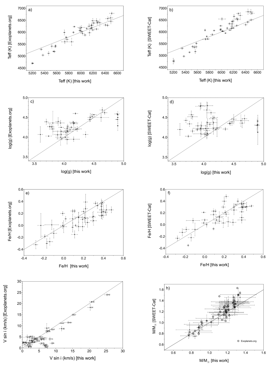
Figure 5: Comparison of our results with those in Exoplanets.org (left) and SWEET-Cat (right): a) and b) $T_{eff}$, c) and d) $\log g$, e) and f) $[Fe/H]$ g) $V\sin i$ h) the mass of the stars, $M_{*}$, with data for Exoplanets.org included.

Another way to verify the consistency of our data is to compare our results with those published in Exoplanets.org (on the left in Fig. 5) and SWEET-Cat (on the right). Taken as a whole, our results seem compatible with the data reported in these two catalogs (note that the uncertainties are those of iSpec), although there are also slight notable differences. In Fig. 5a, our values for $T_{eff}$ are slightly higher below 5800 K than the values reported by Exoplanets.org and SWEET-Cat. However, above 6000 K our temperatures are comparable with those in Exoplanets.org, while clearly lower compared to SWEET-Cat. The largest difference between our results and those of the two other surveys is for $\log g$. Compared with Exoplanets.org (Fig. 5c), our values for $\log g$ are comparable within the range 4-4.7 dex, only slightly underestimated. Above 4.7 dex, our values tend to be overestimated while below 4 dex they are underestimated. These differences are amplified comparing with SWEET-Cat in Fig. 5d. Once again, however, we must conclude that these differences already existed comparing Exoplanets.org with SWEET-Cat. Despite the above differences, our metallicities in Fig. 5e and Fig. 5f are comparable with those published both by Exoplanets.org and SWEET-Cat. Once against our results seem more similar to the former than the latter.

The most important comparison for the purpose of our survey is for $V\sin i$ in Fig. 5g. Unfortunately, we can only compare with Exoplanets.org, since SWEET-Cat did not publish their results. What we find is a very good agreement, with only a slight trend for our values to be higher. This trend is most probably due to our lower resolution and the different way we determined $V_{mic}$ and $V_{mac}$ (more about that will be said later). In Fig. 5h we compare the masses of the stars as compare to those reported by SWEET-Cat. This time we observe a much better consistency. Note that we have also included the values given by Exoplanets.org (as open circles). In general, our masses show a weak trend to be lower, although well within the uncertainties.

To quantify the differences between our values and those reported in Exoplanets.org and SWEET-Cat we compare in Table 5 the medians and means (note that since the numbers of stars in the comparisons vary the means and medians are not the same). In both cases, we also determined if the differences are statistically significant, using non-parametric Mann-Whitney tests (Dalgaard, 2008). The last two columns in Table 5 report the p-values of the tests and the level of significance of the differences (at a level of confidence of 95%). As one can see, the only parameter distributions that are significantly different are the surface gravity, which is slightly lower in our work compared than in Exoplanets.org and SWEET-Cat. The statistical test also confirms that the difference is more significant comparing our data with SWEET-Cat than with Exoplanets.org (p-value   0.0008 instead of 0.0195). Considered as a whole, therefore, these tests suggest that our results are quite comparable with those reported in the literature.

Table 5: Comparison with literature

		TIGRE (45 stars)			Exoplanets			p-value	s.l.
Parameter	Units	median	mean		median	mean
$T_{eff}$	(K)	$6025$	$5975$		$6095$	$5952$		$0.7679$	ns
$\log g$		$4.06$	$4.18$		$4.26$	$4.28$		$0.0195$	*
$[Fe/H]$		$0.07$	$0.12$		$0.20$	$0.18$		$0.1638$	ns
$V\sin i$	(km/s)	$5.55$	$7.39$		$4.10$	$6.92$		$0.2732$	ns
$M_{*}$	(M⊙)	$1.18$	$1.13$		$1.22$	$1.19$		$0.1010$	ns
$R_{*}$	(R⊙)	$1.57$	$1.47$		$1.34$	$1.36$		$0.0868$	ns
		TIGRE (44 stars)			SWEET-Cat			p-value	s.l.
Parameter	Units	median	mean		median	mean
$T_{eff}$	(K)	$6046$	$5977$		$6133$	$6036$		$0.2936$	ns
$\log g$		$4.06$	$4.18$		$4.33$	$4.34$		$0.0008$	***
$[Fe/H]$		$0.08$	$0.12$		$0.20$	$0.17$		$0.1973$	ns
$M_{*}$	(M⊙)	$1.18$	$1.13$		$1.24$	$1.18$		$0.0700$	ns

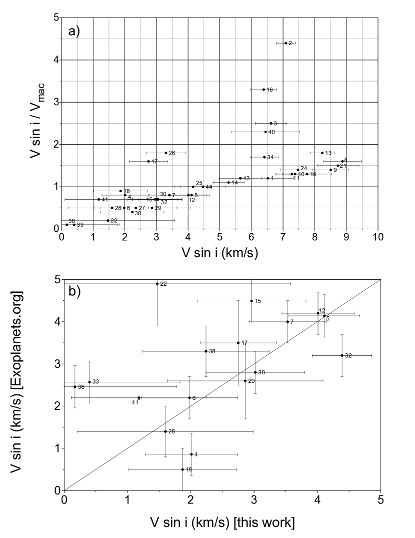
Figure 6: a) The ratio $V\sin i/V_{mac}$ as a function of $V\sin i$. Below $V\sin i=4$ the ratios are lower than 1. Three stars, 33, 36 and 22 have iSpec have values with uncertainties that include zero. b) Zoom of the region in Fig. 5g with $V\sin i<5$ km/s.

As we mentioned before, as the temperature of the stars goes down, $V_{mic}$ and $V_{mac}$ become comparable to $V\sin i$ and thus it is more complicated to separated one from the others. In Valenti & Fischer (2005) spectral synthesis analysis, the authors recognized this problem stating, in particular, that, “…adopting a global macroturbulence relationship should yield more accurate results than solving for $V_{mac}$ in each individual spectrum.” To determine such relation they fixed $V\sin i=0$, obtaining the maximum values $V_{mac}$ could have at different temperatures. Note that these authors did not report any dependence on the spectral resolution, although they used spectra with R between 50,000 and almost 100,000. The maximum relation they deduced can be seen in Fig. 4. According to these authors, below $T_{eff}=5800$ K $V\sin i$ becomes negligible, and what we measure then must be the “real” $V_{mac}$. However, this conclusion contradicts what was expected based on the semi-empirical relation established by Gray (1984b) and later the minimum relation for $V_{mac}$ obtained by Bruntt et al. (2010) by line modeling (the two relations can also be seen in Fig. 4). These results suggest that applying the right macro (and micro) turbulence relationship one could obtain a value of $V\sin i\neq 0$ below $T_{eff}=5800$ K. In fact, in our analysis of the Sun, we did reproduced the value of $V\sin i$, using the relation for $V_{mic}$ obtained by Tsantaki et al. (2014) and $V_{mac}$ determined by Doyle et al. (2014), both depending not only on $T_{eff}$ but also on on $\log g$, and where $V\sin i<V_{mac}$. The question then is how low can $V\sin i$ be compared to $V_{mac}$ and still be distinguishable by iSpec?

In Fig. 6a, we compare $V\sin i$ with the ratio $V\sin i/V_{mac}$. What we observe is that below $V\sin i=4$ km/s the ratio is lower than one. As one can see in Fig.4, a value of $V_{mac}=4$ km/s ($V\sin i/V_{mac}=1$) corresponds to $T_{eff}\sim 5800$ K. Therefore, our results are at the same time consistent with the conclusion of Valenti & Fischer (2005), since below $T_{eff}=5800$ K $V\sin i$ is lower than $V_{mac}$, and consistent with Gray (1984a), Bruntt et al. (2010) and Doyle et al. (2014), since $V\sin i\neq 0$. But how low could a value of $V\sin i$ below $V_{mac}$ be? This question we already answered in Fig. 5g where we compared our values of $V\sin i$ with the values reported by Exoplanets.org. To get a better view, in Fig. 6b we zoom in on values of $V\sin i\leq 5$ km/s. Except for three stars, 22, 33 and 36, with $V\sin i/V_{mac}<0.4$, all the other stars have $V\sin i$ comparable to the values reported in Exoplanets.org (in fact, two of the stars, 4 and 16, have higher values). In Fig. 6a note that the iSpec uncertainty increases as $V\sin i$ goes down. As a consequence, the possible values for the stars 22, 33 and 36 include zero. However, could stars with $V\sin i=0$ exist physically? Considering that the loss of angular momentum plays an important role in the formation of stars this would seem difficult to explain (note that we did obtained $V\sin i=0$ for some stars in our initial list, but they were not included in our study). Since Gray (1984b) study the problem seems clear: how can we measure the rotation of a star where $V_{mac}$ is as high or even higher than $V\sin i$? It seems that the best approach is assuming an a priori global relation and see what comes out from the residual (Gray, 1984a, b; Fischer & Valenti, 2005; Bruntt et al., 2010; Tsantaki et al., 2014; Doyle et al., 2014). However, to stay safe, due to their higher uncertainties we should not consider 22, 33 and 36 in our statistical analysis for $V\sin i$.

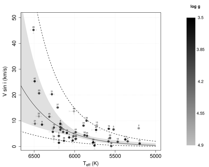
Figure 7: Exponential relation between the rotational velocity, the temperature and the surface gravity for the 46 stars in our sample. The black triangle represent the Sun. The gray area corresponds to the interval of confidence and the dashed curves delimit the prediction interval.

Considering the results above, one expects the rotational rotation to decrease with the temperature, but still be above zero in cool stars. Moreover, since Tsantaki et al. (2014) and Doyle et al. (2014) have found relations for $V_{mic}$ and $V_{mac}$ that depend not only on $T_{eff}$ but also on on $\log g$, we might expect a similar relation for $V\sin i$, $T_{eff}$ and $\log g$. In Fig. 7, we show the diagram of $V\sin i$ and $T_{eff}$ for our stars. The dependence in $\log g$ is shown by the gray-scale bar. In Fig. 7, we also traced over our data the bi-exponential relation we obtained, together with the interval of confidence (in gray) and the prediction interval (dashed curves), which takes into account the uncertainty of each measurement. The final relation we obtained is the following:

$$\frac{V\sin i}{\rm km/s}=\exp\left[\ A\left(\frac{T_{eff}}{1000{\rm K}}\right)+B\log g-C\ \right]$$ (7)

where $A=2.20\pm 0.36$, $B=0.30\pm 0.46$ and $C=12.91\pm 3.59$, and which has a multiple correlation coefficient of $r^{2}=0.6329$. Except for the stars 2, 3, 13 and 16, and the three stars with highest uncertainties (22, 33, and 36; not considered in this relation) all our data fit well inside the prediction interval.

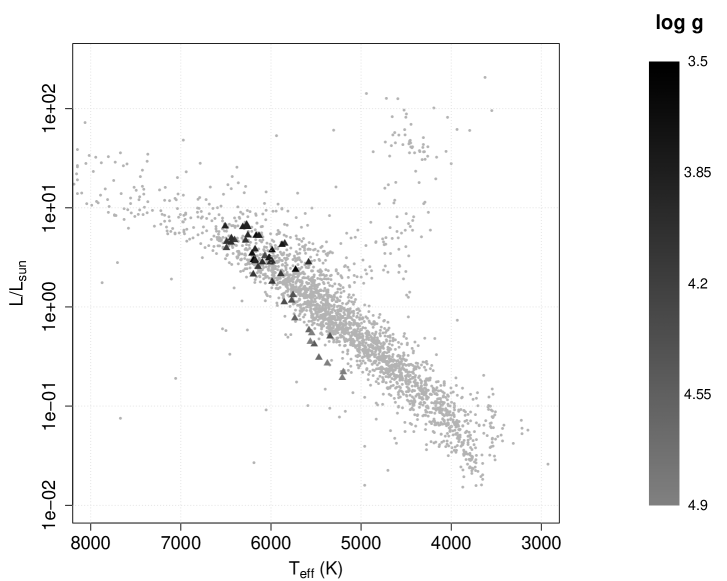
Figure 8: HR diagram of our 46 stars, overlayed on the main sequence of Hipparchos stars.

Note that in order to obtain the highest correlation coefficient possible, 8 stars suspected to have peculiarly high rotation for their temperature were considered as outliers. They are, from right to left in Fig. 7: 2, 3, 16, 13, 40, 39, 46 and 37. Different reasons were explored that could explain why these stars would be outliers. One is the age of the stars (e.g., Stauffer & Hartman, 1986), younger stars rotating faster than older stars (see Fig. 1.6 in Tassoul, 2000). In Tassoul (2000) it was also shown that young stars trace the same relation of $V\sin i$ with $T_{eff}$ as old stars, with only higher velocities, forming an upper sequence (or upper envelope). This could be what we see in Fig. 7. However, in Fig. 8 the HR diagram for our stars compared to Hipparchos stars suggests that, except for three stars with slightly higher luminosity for their temperature (6, 25 and 32; none of these stars forming the envelope) all of the stars more luminous than the Sun are clearly on the main sequence. This eliminates the young age hypothesis. Another explanation could be peculiar surface activity. Since more than one phenomena can cause such activities, the expected effect would be pure random dispersion. Revising the literature for each of the star in our sample we did find 8 stars with reported peculiarities: 2, 3, 17, 26, 33, 37, 39 and 46. The type of peculiarities encountered included, “Flare star”, “Rotationally variable”, “Variable BY DRa”, and “Double or Multiple star”. Of these“active” stars only five in Fig. 7 have an higher $V\sin i$ for their temperature: 2, 3, 37, 39 and 46. This left three stars (13, 16 and 40) with unexplained, relatively high $V\sin i$ values. In fact, checking their $V_{mac}$ we found these stars have lower values than stars with comparable temperatures. However, in our various attempts to get the higher highest correlation coefficient possible, we judged better to keep them as outliers.

Figure 9: Data as found in Exoplanets.org.

To verify our relation, in Fig. 9 we traced it over the distribution of the rotational velocities and temperatures of the stars that were in our initial sample based on Exoplanets.org. As one can see, except for a few stars below $T_{eff}=5500$ K, with higher velocities, and stars below $T_{eff}=5500$ K, with lower velocities (some with $V\sin i=0$) the majority of the stars in this sample fall well between the prediction interval of our empirical relation. This result suggests that the decrease in angular momentum of low mass stars is a non-aleatory phenomenon, most probably reflecting the action of one specific mechanism, like, for example, magnetic braking or stellar wind (Wolff & Simon, 1997; Tassoul, 2000; Uzdensky et al., 2002). An exciting possibility, however, could be that this relation somehow is coupled to the formation of the planets. Although this hypothesis proposed in the late 1960s was rapidly rejected, since no planet out of the solar system was known at the time, the discovery of exoplanets allows us today to test this idea anew (e.g., Berget & Durrance, 2010). This will be the subject of Paper II, in search of a connection between the formation of stars and planets.

0.5 Conclusions

In this study we have shown that our method of analysis developed for the TIGRE telescope using iSpec on intermediate Echelle resolution spectra yields results about the physical characteristics of stars, host of exoplanets, that are comparable to those obtained using bigger telescopes and standard spectra analysis methods, using high resolution spectra. Our results show that TIGRE can have an helpful contribution in the follow up of exoplanet surveys around bright stars, like TESS and PLATO. Such follow up studies are essential in order to understand how the formation of planets is connected to the formation of their host stars (Eisner et al., 2020).

0.6 List of spectral lines and segments defined for our analysis

Table 6: Lines and segments defined in this work.

Line	Wave Peak	Wave Base	Wave Top	Segm. Wave base	Segm. Wave top
Na 1	588.9959	588.9422	589.0422	588.8922	589.0922
Na 1	589.5916	589.5411	589.6411	589.4911	589.6911
Fe 1	593.0186	592.9859	593.0539	592.9359	593.1039
Fe 1	593.4665	593.4289	593.5059	593.3789	593.5559
No ident.	595.6706	595.6206	595.7206	595.5706	595.7706
Fe 1	597.5341	597.4898	597.5898	597.4398	597.7729
Fe 1	597.6777	597.6299	597.7229	-	-
Fe 1	598.4831	598.4319	598.5689	598.3819	598.8099
Fe 1	598.7088	598.6449	598.7599	-	-
Fe 1	600.2986	600.2519	600.3509	600.2019	600.4009
Fe 1	600.8552	600.8249	600.8989	600.7749	600.9489
Mn 1	601.6628	601.6110	601.7110	601.5610	601.7610
Fe 1	602.0142	601.9637	602.0637	601.9137	602.1137
Fe 1	602.4066	602.3579	602.4639	602.3079	602.5139
Fe 1	605.6032	605.5599	605.6809	605.5099	605.7309
Fe 1	606.5494	606.5009	606.5919	606.4509	606.6419
Fe 1	607.8490	607.7729	607.8769	607.7229	607.9269
Fe 1	608.2757	608.2180	608.3180	608.1680	608.3680
Fe 1	608.5228	608.4775	608.5775	608.4275	608.6275
Ca 1	612.2225	612.1703	612.2703	612.1203	612.3203
No ident.	615.1608	615.1108	615.2108	615.0608	615.2608
Ca 1	616.2171	616.1690	616.2690	616.1190	616.3190
Fe 1	617.0503	617.0028	617.1168	616.9528	617.1668
Fe 1	617.3340	617.2828	617.3838	617.2328	617.4338
Fe 1	621.3421	621.2988	621.3958	621.2488	621.4458
Fe 1	621.9270	621.8418	621.9698	621.7918	622.0198
Fe 1	623.0722	623.0278	623.1868	622.9778	623.3578
Fe 1	623.2644	623.1868	623.3078	-	-
Fe 1	624.6326	624.5898	624.6868	624.5398	624.7368
Fe 1	625.2564	625.2108	625.3108	625.1608	625.7298
Fe 1	625.4240	625.3298	625.5098	-	-
Fe 1	625.6343	625.5628	625.6798	-	-
Fe 1	629.0951	629.0473	629.1473	628.9973	629.1973
Fe 1	629.7808	629.7138	629.8548	629.6638	629.9048
Fe 1	630.1508	630.0898	630.2028	630.0398	630.3528
Fe 1	630.2514	630.2028	630.3028	-	-
Fe 1	632.2710	632.2228	632.3128	632.1728	632.3628
Fe 1	633.5331	633.4658	633.5888	633.4158	633.7978
Fe 1	633.6827	633.6388	633.7478	-	-
Fe 1	635.5038	635.4468	635.5768	635.3968	635.6268
Fe 1	635.8671	635.8128	635.9258	635.7628	635.9758
Fe 1	638.0743	638.0264	638.1264	637.9764	638.1764
Fe 1	639.3612	639.2968	639.4278	639.2468	639.4778
Fe 1	640.8011	640.7578	640.9138	640.7078	640.9638
Fe 1	641.1646	641.0878	641.2198	641.0378	641.2698
Fe 2	641.6962	641.6449	641.7449	641.5949	641.7949
Fe 1	641.9949	641.9428	642.0408	641.8928	642.2598
Fe 1	642.1377	642.0758	642.2098	-	-
Fe 1	643.0851	643.0158	643.1528	642.9658	643.3681
Fe 2	643.2663	643.2181	643.3181	-	-
Ca 1	643.9063	643.8572	643.9572	643.8072	644.0072
Fe 2	645.6405	645.5866	645.6866	645.5366	645.7366
Ca 1	646.2606	646.2081	646.3081	646.1581	646.3581
Fe 1	646.9200	646.8711	646.9711	646.8211	647.0211
Fe 1	647.5657	647.5117	647.6117	647.4617	647.6617
Fe 1	648.1882	648.1362	648.2362	648.0862	648.2862
Fe 1	649.4989	649.4197	649.5437	649.3697	649.5937
Fe 2	651.6098	651.5587	651.6587	651.5087	651.7087
Fe 1	651.8385	651.7868	651.8868	651.7368	651.9368
Fe 1	654.6245	654.5757	654.6967	654.5257	654.7467
H 1	656.2808	655.5483	656.6832	655.1934	656.7340
Fe 1	657.5003	657.4507	657.5507	657.4007	657.6007
Fe 1	659.3887	659.3417	659.4537	659.2917	659.5037
Fe 1	659.7585	659.7073	659.8073	659.6573	659.8573
Fe 1	660.9067	660.8605	660.9605	660.8105	661.0105
Ni 1	664.3626	664.3139	664.4139	664.2639	664.4639
Fe 1	667.7983	667.7297	667.8707	667.6797	667.9207
Fe 1	670.5134	670.4570	670.5570	670.4070	670.6070
No ident.	671.3073	671.2573	671.3573	671.2073	671.4073
Ca 1	671.7701	671.7138	671.8138	671.6638	671.8638
Fe 1	672.6657	672.6178	672.7178	672.5678	672.7678
Fe 1	675.0182	674.9653	675.0653	674.9153	675.1153
Fe 1	680.6856	680.6358	680.7358	680.5858	680.7858
Fe 1	682.0359	681.9894	682.0894	681.9394	682.1394
Fe 1	682.8620	682.8085	682.9085	682.7585	682.9585
No ident.	683.9811	683.9311	684.0311	683.8811	684.0811
Fe 1	684.3658	684.3150	684.4150	684.2650	684.4650
Fe 1	691.6669	691.6218	691.7218	691.5718	691.7718
No ident.	693.3635	693.3135	693.4135	693.2635	693.4635
Fe 1	694.5196	694.4703	694.5703	694.4203	694.6203
-	-	-	-	694.6410	694.8410
Fe 1	695.1251	695.0721	695.1721	695.0221	695.2221
Fe 1	703.8209	703.7718	703.8718	703.7218	703.9218
Fe 1	706.8440	706.7918	706.8918	706.7418	706.9418
Fe 1	709.0378	708.9850	709.0850	708.9350	709.1350
Fe 1	713.0900	713.0451	713.1451	712.9951	713.1951
Fe 1	713.3001	713.2453	713.3453	713.1953	713.3953
CN 1	714.5241	714.4768	714.5768	714.4268	714.6268
Ca 1	714.8155	714.7666	714.8666	714.7166	714.9166
Fe 1	715.5670	715.5125	715.6125	715.4625	715.6625
No ident.	716.4473	716.3185	716.5085	716.2685	716.5585
Fe 1	717.5970	717.5403	717.6403	717.4903	717.6903
Fe 1	721.9712	721.9134	722.0134	721.8634	722.2190
CN 1	722.1100	722.0690	722.1690	-	-
No ident.	724.4812	724.4312	724.5312	724.3812	724.5812
Fe 1	732.0693	732.0178	732.1178	731.9678	732.1678
Fe 1	738.6353	738.5818	738.6818	738.5318	738.7318
Fe 1	738.9363	738.8454	738.9974	738.7954	739.0474
Fe 1	741.1151	741.0394	741.1764	740.9894	741.2264
Ni 1	742.2264	742.1770	742.2770	742.1270	742.3270
No ident.	744.0877	744.0377	744.1377	743.9877	744.1877
Fe 1	744.5740	744.5174	744.6654	744.4674	744.7154
Fe 1	749.5088	749.4484	749.5724	749.3984	749.6224
Fe 1	751.1024	751.0024	751.1854	750.9524	751.2354
Fe 1	771.0389	770.9827	771.0827	770.9327	771.1327
Fe 1	772.3237	772.2724	772.3724	772.2224	772.4224
Fe 1	774.8304	774.7653	774.8613	774.7153	774.9113
Ni 1	775.1163	775.0625	775.1625	775.0125	775.2125
Fe 1	778.0562	777.9613	778.1263	777.9113	778.1763
Fe 1	783.2221	783.1453	783.3183	783.0953	783.3683
Fe 1	793.7145	793.6112	793.7802	793.5612	793.8302
Fe 1	794.5839	794.5132	794.6502	794.4632	794.7002
Fe 1	799.8967	799.8112	799.9622	799.7612	800.0122
No ident.	804.6052	804.5282	804.7002	804.4782	804.7502
No ident.	808.5170	808.4442	808.6012	808.3942	808.6512
Fe 1	820.7791	820.7284	820.8284	820.6784	820.8784
Fe 1	832.7062	832.6341	832.7711	832.5841	832.8211
Fe 1	838.7760	838.7061	838.8521	838.6561	838.9021
Fe 1	846.8392	846.7820	846.8930	846.7320	846.9430
Fe 1	851.4073	851.3290	851.4650	851.2790	851.5150
Fe 1	868.8639	868.7760	868.9430	868.7260	868.9930
No ident.	871.0395	870.9895	871.0895	870.9395	871.1395

References

- Anand et al. (2004) Anand M., Bland P., McBride N., Moore E. A., Rothery D. A., Schwenzer S. P., Widdowson M., Wright I., 2004, An Introduction to the Solar System. http://dx.doi.org/doi:10.2277/0521546206
- Anderson et al. (2014) Anderson, D. R., Collier Cameron, A., Delrez, L., et al. 2014, MNRAS, 445, 1114
- Armitage (2020) Armitage P. J., 2020, Astrophysics of planet formation, 2nd Ed. Cambridge University Press
- Asplund et al. (2009) Asplund M., Grevesse N., Sauval A. J., Scott P., 2009, Astrophysics and Space Science, 328, 179
- Bakos et al. (2007) Bakos, G. Á., Kovács, G., Torres, G., et al. 2007, ApJ, 670, 826
- Bakos et al. (2012) Bakos, G. Á., Hartman, J. D., Torres, G., et al. 2012, AJ, 144, 19
- Barros et al. (2011) Barros, S. C. C., Faedi, F., Collier Cameron, A., et al. 2011, A&A, 525, A54
- Baruteau et al. (2014) Baruteau, C., Crida, A., Paardekooper, S.-J., et al. 2014, Protostars and Planets VI, 667
- Batalha et al. (2013) Batalha, N. M., Rowe, J. F., Bryson, S. T., et al. 2013, ApJS, 204, 24
- Beatty et al. (2012) Beatty, T. G., Pepper, J., Siverd, R. J., et al. 2012, ApJ, 756, L39
- Berget & Durrance (2010) Berget D. J., Durrance S. T., 2010, Journal of the Southeastern Association for Research in Astronomy, 3, 32
- Beaugé & Nesvorný (2012) Beaugé, C., & Nesvorný, D. 2012, ApJ, 751, 119
- Bieryla et al. (2015) Bieryla, A., Collins, K., Beatty, T. G., et al. 2015, AJ, 150, 12
- Blanco-Cuaresma (2014) Blanco-Cuaresma S., Soubiran C., Heiter U., Jofré P., 2014, A& A, 569,A111
- Blanco-Cuaresma (2019) Blanco-Cuaresma S., 2019, MNRAS, 486, 2075
- Bouchy et al. (2005) Bouchy, F., Udry, S., Mayor, M., et al. 2005, A&A, 444, L15
- Borucki et al. (2011) Borucki, W. J., Koch, D. G., Basri, G., et al. 2011, ApJ, 736, 19
- Boss (1997) Boss A. P., 1997, Science, 276, 1836
- Butler et al. (2000) Butler, R. P., Vogt, S. S., Marcy, G. W., et al. 2000, ApJ, 545, 504
- Bruntt et al. (2010) Bruntt, H., Bedding, T. R., Quirion, P.-O., et al. 2010, MNRAS, 405, 1907
- Chabrier et al. (2009) Chabrier G., Baraffe I., Leconte J., Gallardo J., Barman T., 2009, AIP Conference Proceedings, 1094, 102
- Charbonneau et al. (2000) Charbonneau, D., Brown, T. M., Latham, D. W., et al. 2000, ApJ, 529, L45
- Chatterjee et al. (2008) Chatterjee, S., Ford, E. B., Matsumura, S., et al. 2008, ApJ, 686, 580
- Chiang & Laughlin (2013) Chiang, E., & Laughlin, G. 2013, MNRAS, 431, 3444
- da Silva et al. (2006) da Silva, R., Udry, S., Bouchy, F., et al. 2006, A&A, 446, 717
- Dalgaard (2008) Dalgaard, P., 2008, Introductory statistics with R, Springer, Berlin, doi:10.1007/978-0-387-79054-1
- Damasso et al. (2015) Damasso, M., Esposito, M., Nascimbeni, V., et al. 2015, A&A, 581, L6
- Dawson & Johnson (2018) Dawson, R. I., & Johnson, J. A. 2018, ARA&A, 56, 175
- Doyle et al. (2014) Doyle A. P., Davies G. R., Smalley B., Chaplin W. J., Elsworth Y., 2014, MNRAS, 444, 3592
- Eisner et al. (2020) Eisner, N. L., Barragán, O., Aigrain, S., et al. 2020, MNRAS, 148
- Fischer et al. (2005) Fischer, D. A., Laughlin, G., Butler, P., et al. 2005, ApJ, 620, 481
- Fischer & Valenti (2005) Fischer D. A., Valenti J., 2005, ApJ, 622, 1102
- Fischer et al. (2006) Fischer, D. A., Laughlin, G., Marcy, G. W., et al. 2006, ApJ, 637, 1094
- Fischer et al. (2007) Fischer, D. A., Vogt, S. S., Marcy, G. W., et al. 2007, ApJ, 669, 1336
- Gandolfi et al. (2017) Gandolfi D., et al., 2017, AJ, 154, 123
- Gray (1984a) Gray D. F., 1984a, ApJ, 277, 640
- Gray (1984b) Gray D. F., 1984b, ApJ, 281, 719
- Gray & Corbally (1994) Gray, R. O., & Corbally, C. J. 1994, AJ, 107, 742
- Han et al. (2014) Han E., Wang S. X., Wright J. T., Feng Y. K., Zhao M., Fakhouri O., Brown J. I., Hancock C., 2014, PASP, 126, 827
- Hellier et al. (2015) Hellier, C., Anderson, D. R., Collier Cameron, A., et al. 2015, AJ, 150, 18
- Hempelmann et al. (2016) Hempelmann A., Mittag M., Gonzalez-Perez J. N., Schmitt J. H. M. M., Schröder K. P., Rauw G., 2016, A& A, 586, A14
- Henry et al. (2000) Henry, G. W., Marcy, G. W., Butler, R. P., et al. 2000, ApJ, 529, L41
- Herbst et al. (2007) Herbst W., Eisloeffel J., Mundt R., Scholz A., , in , Protostars and Planets V, B. Reipurth, D. Jewitt, and K. Keil (eds.), 2007, University of Arizona Press, Tucson, 951. pp 297-311 (arXiv:0603673)
- Hestroffer & Magnan (1998) Hestroffer D., Magnan C., 1998, A& A, 333, 338
- Hinkel et al. (2014) Hinkel, N. R., Timmes, F. X., Young, P. A., et al. 2014, AJ, 148, 54
- Hinkel et al. (2016) Hinkel, N. R., Young, P. A., Pagano, M. D., et al. 2016, ApJS, 226, 4
- Howard et al. (2011) Howard, A. W., Johnson, J. A., Marcy, G. W., et al. 2011, ApJ, 730, 10
- Irwin (2015) Irwin S. A., 2015, PhD Thesis, College of Science at Florida Institute of Technology
- Jófre et al. (2017) Jofré, P., Heiter, U., Soubiran, C., et al. 2014, A&A, 564, A133
- Johns-Krull et al. (2008) Johns-Krull, C. M., McCullough, P. R., Burke, C. J., et al. 2008, ApJ, 677, 657
- Johnson et al. (2006) Johnson, J. A., Marcy, G. W., Fischer, D. A., et al. 2006, ApJ, 647, 600
- Johnson et al. (2011) Johnson, J. A., Winn, J. N., Bakos, G. Á., et al. 2011, ApJ, 735, 24
- Joshi et al. (2009) Joshi, Y. C., Pollacco, D., Collier Cameron, A., et al. 2009, MNRAS, 392, 1532
- Kraft (1967) Kraft R. P., 1967, ApJ, 150, 551
- Kupka et al. (1999) Kupka F., Piskunov N., Ryabchikova T. A., Stempels H. C., Weiss W. W., 1999, A& AS, 138, 119
- Kupka et al. (2011) Kupka F., Dubernet P. I., 2011, Baltic Astronomy, 20, 503
- Kurucz (2005) Kurucz R. L., 2005, Memorie della Società Astronomica Italiana Supplement, 8, 14
- Kuzuhara et al. (2013) Kuzuhara, M., Tamura, M., Kudo, T., et al. 2013, ApJ, 774, 11
- Latham et al. (2009) Latham, D. W., Bakos, G. Á., Torres, G., et al. 2009, ApJ, 704, 1107
- Leconte et al. (2009) Leconte J., Baraffe I., Chabrier G., Barman T. S., Levrard 2009, A& A, 506, 385
- Lee et al. (2017) Lee E. J., Chiang E., 2017, ApJ, 842, 40
- Lin et al. (1996) Lin, D. N. C., Bodenheimer, P., & Richardson, D. C. 1996, Nature, 380, 606
- Luhman et al. (2007) Luhman, K. L., Patten, B. M., Marengo, M., et al. 2007, ApJ, 654, 570
- Marcy et al. (2000) Marcy, G. W., Butler, R. P., & Vogt, S. S. 2000, ApJ, 536, L43
- Marcy et al. (2002) Marcy, G. W., Butler, R. P., Fischer, D. A., et al. 2002, ApJ, 581, 1375
- Martin & Livio (2012) Martin R. G., & Livio M., 2012, MNRAS: Letters, 425, L6
- Martin & Livio (2015) Martin R. G., Livio M., 2015, ApJ, 810, 105
- Marzari & Weidenschilling (2002) Marzari, F., & Weidenschilling, S. J. 2002, Icarus, 156, 570
- Mayor & Queloz (1995) Mayor, M., & Queloz, D. 1995, Nature, 378, 355
- McKee & Ostriker (2007) McKee, C. F., & Ostriker, E. C. 2007, ARA&A, 45, 565
- McNally (1965) McNally D., 1965, The Observatory, 85, 166
- Mittag et al. (2016) Mittag M., Schröder K.-P., Hempelmann A., González-Pérez J. N., Schmitt J. H. M. M., 2016, A& A, 591, A89
- Motalebi et al. (2015) Motalebi, F., Udry, S., Gillon, M., et al. 2015, A&A, 584, A72
- Nagasawa et al. (2008) Nagasawa, M., Ida, S., & Bessho, T. 2008, ApJ, 678, 498
- Neveu-VanMalle et al. (2014) Neveu-VanMalle, M., Queloz, D., Anderson, D. R., et al. 2014, A&A, 572, A49
- Noyes et al. (2008) Noyes, R. W., Bakos, G. Á., Torres, G., et al. 2008, ApJ, 673, L79
- Nomura et al. (2016) Nomura, H., Tsukagoshi, T., Kawabe, R., et al. 2016, ApJ, 819, L7
- Moutou et al. (2005) Moutou, C., Mayor, M., Bouchy, F., et al. 2005, A&A, 439, 367
- Pál et al. (2008) Pál, A., Bakos, G. Á., Torres, G., et al. 2008, ApJ, 680, 1450
- Pepper et al. (2013) Pepper, J., Siverd, R. J., Beatty, T. G., et al. 2013, ApJ, 773, 64
- Pérez et al. (2019) Pérez S., Casassus S., Baruteau C., Dong R., Hales A., Cieza L., 2019, AJ, 158, 15
- Piskunov & Valenti (2017) Piskunov, N. & Valenti, J. A. 2017, A&A, 597, A16
- Plummer et al. (2005) Plummer C. C., Carlson D. H., Hammersley L., 2005, Physical geology
- Queloz et al. (2010) Queloz, D., Anderson, D. R., Collier Cameron, A., et al. 2010, A&A, 517, L1
- Rasio & Ford (1996) Rasio, F. A., & Ford, E. B. 1996, Science, 274, 954
- Raymond et al. (2008) Raymond, S. N., Barnes, R., & Mandell, A. M. 2008, MNRAS, 384, 663
- Raymond & Morbidelli (2020) Raymond, S. N., & Morbidelli, A. 2020, arXiv e-prints, arXiv:2002.05756
- Radick et al. (1987) Radick R. R., Thompson D. T., Lockwood G. W., Duncan D. K., Baggett W. E., 1987, ApJ, 321, 459
- Sato et al. (2005) Sato, B., Fischer, D. A., Henry, G. W., et al. 2005, ApJ, 633, 465
- Schmitt et al. (2014) Schmitt J. H. M. M., et al., 2014, Astronomische Nachrichten, 335, 787
- Schneider et al. (2011) Schneider J., Dedieu C., Le Sidaner P., Savalle R. & Zolotukhin I. 2011, A&A, 532, A79
- Seager (2010) Seager S., 2010, Exoplanets. http://adsabs.harvard.edu/abs/2010exop.book....S
- Skillen et al. (2009) Skillen, I., Pollacco, D., Collier Cameron, A., et al. 2009, A&A, 502, 391
- Skumanich (1972) Skumanich A., 1972, ApJ, 171, 565
- Smalley et al. (2011) Smalley, B., Anderson, D. R., Collier Cameron, A., et al. 2011, A&A, 526, A130
- Smette et al. (2015) Smette, A., Sana, H., Noll, S., et al. 2015, A&A, 576, A77
- Sousa et al. (2008) Sousa, S. G., Adibekian, V., Delgado-Mena, E., et al. 2008, A&A, 620, A58
- Stauffer & Hartman (1986) Stauffer J. R., Hartman L. W., 1986, PASP, 98, 1233
- Tassoul (2000) Tassoul J.-L., 2000, Stellar Rotation. Cambridge University Press, Cambridge, doi:10.1017/CBO9780511546044
- Torres et al. (2010) Torres, G., Bakos, G. Á., Hartman, J., et al. 2010, ApJ, 715, 458
- Tsantaki et al. (2014) Tsantaki M., Sousa S. G., Santos N. C., Montalto M., Delgado-Mena E., Mortier A., Adibekyan V., Israelian G., 2014, A& A, 570, A80
- Udry et al. (2000) Udry, S., Mayor, M., Naef, D., et al. 2000, A&A, 356, 590
- Udry & Santos (2007) Udry, S., & Santos, N. C. 2007, ARA&A, 45, 397
- Uzdensky et al. (2002) Uzdensky D. A., Konigl A., Litwin C., 2002, ApJ, 565, 1191
- Valencia et al. (2006) Valencia, D., O’Connell, R.J., & Sasselov, D. 2006, Icarus, 181, 545
- Valenti & Fischer (2005) Valenti, J. A., & Fischer, D. A. 2005, ApJS, 159, 141
- van der Marel et al. (2018) van der Marel N., Williams J., Bruderer S., 2018, ApJ Letters, 867, L14
- Walsh et al. (2011) Walsh, K. J., Morbidelli, A., Raymond, S. N., et al. 2011, Nature, 475, 206
- Wang & Zhong (2018) Wang, J., & Zhong, Z. 2018, A&A, 619, L1
- Weidenschilling & Marzari (1996) Weidenschilling, S. J., & Marzari, F. 1996, Nature, 384, 619
- West et al. (2016) West, R. G., Hellier, C., Almenara, J.-M., et al. 2016, A&A, 585, A126
- Wilson (1963) Wilson O. C., 1963, ApJ, 138, 832
- Wolff & Simon (1997) Wolff S., Simon T., 1997, PASP, 109, 759