The black hole spin in GRS 1915+105, revisited

Abstract

We estimate the black hole spin parameter in GRS 1915+105 using the continuum-fitting method with revised mass and inclination constraints based on the very long baseline interferometric parallax measurement of the distance to this source. We fit Rossi X-ray Timing Explorer observations selected to be accretion disk-dominated spectral states as described in McClinotck et al. (2006) and Middleton et al. (2006), which previously gave discrepant spin estimates with this method. We find that, using the new system parameters, the spin in both datasets increased, providing a best-fit spin of $a_{*}=0.86$ for the Middleton et al. data and a poor fit for the McClintock et al. dataset, which becomes pegged at the BHSPEC model limit of $a_{*}=0.99$. We explore the impact of the uncertainties in the system parameters, showing that the best-fit spin ranges from $a_{*}=0.4$ to 0.99 for the Middleton et al. dataset and allows reasonable fits to the McClintock et al. dataset with near maximal spin for system distances greater than $\sim 10$ kpc. We discuss the uncertainties and implications of these estimates.

1 Introduction

A soft, apparently thermal emission component is frequently observed in the spectra of black hole candidate X-ray binaries (hereafter BHXRBs) along with a second, harder X-ray component. The soft component is widely believed to be emission from an optically-thick, geometrically thin accretion disk (Shakura & Sunyaev, 1973), while the hard component is thought to be Comptonized emission from hot electrons near the disk (the corona). Most BHXRBs display variability between spectral states where the relative strengths of these components vary, with the high/soft state referring to cases where the disk component dominates (Remillard & McClintock, 2006; Done et al., 2007).

When BHXRBs enter strongly disk-dominated high/soft states, one might expect the emission to be well-represented by a bare accretion disk model, which accounts for the relativistic effects on photon emission and the possible change in flow properties at or near the black hole’s innermost stable circular orbit (ISCO). This has motivated a number of relativistic accretion disk spectral models (Hanawa, 1989; Gierliński et al., 1999; Li et al., 2005; Davis & Hubeny, 2006), which have had success in fitting the spectrum and its variation with accretion rate in the high/soft state of many BHXRBs (Gierliński & Done, 2004; Davis et al., 2005; Shafee et al., 2006; McClintock et al., 2011). Placing constraints on the black hole angular momentum, or spin, is a key motivation of many such studies (for a review, see Middleton, 2016). The spectrum of the disk is sensitive to the spin through location of the ISCO as well as the relativistic effects on the photon propagation through the black hole spacetime. This technique of spin measurement is generally referred to as the continuum-fitting method (Zhang et al., 1997; McClintock et al., 2011), which distinguishes it from other spectral-fitting spin measurements such as those that fit the reflected emission features, including the prominent Fe K$\alpha$ line (Fabian et al., 1989).

The continuum-fitting method has previously been applied to the BHXRB GRS 1915+105, yielding inconsistent estimates for the black hole spin (McClintock et al., 2006; Middleton et al., 2006). Although these studies used similar spectral models and fitting methods, Middleton et al. (2006) (hereafter MID06) found a more moderate spin parameter ($a_{*}\sim 0.7$) while McClintock et al. (2006) (hereafter MCC06) favored high spin ($a_{*}\gtrsim 0.98$), where we define the dimensionless spin parameter $a_{*}=Jc/(GM^{2})$ and $J$ is the angular momentum of the black hole. This discrepancy in spin can be primarily attributed to differences in the selection of spectra used in their analyses. These differences arise from the difficulties in unambiguously identifying a disk-dominated state in this source, which is famous for its complex variability, with a diversity not generally seen in other low mass X-ray binaries (Belloni et al., 2000) except for the black hole source IGR J17091-3624 (Altamirano et al., 2011).

Both studies focused on analysis of spectral observations using data taken by the PCA detector on board the Rossi X-Ray Timing Explorer (hereafter RXTE). MCC06 identified a selection of apparently disk-dominated spectra in the 3-25 keV range based on a number of screening criteria, including RMS variability and hardness ratio, ultimately arriving at 20 candidates. MID06 argued against identifying the MCC06 sample as disk-dominated, instead arguing these observations are more like very high/steep power law states (Remillard & McClintock, 2006; Done et al., 2007), in which a low temperature Comptonization component is present (Zdziarski et al., 2005, MID06). Instead, MID06 generated a large library of spectra in the 3-20 keV range with 16 second exposures from observations within the $\beta$ and $\kappa$ variability classes of Belloni et al. (2000), ultimately identifying 34 disk-dominated candidates. MCC06, in turn, criticized this selection process, raising concerns about potential systematic errors arising from the short 16 second exposures while also worrying that the implied luminosity of observations were above or sufficiently close to the Eddington limit as to invalidate the assumptions of the underlying disk model. In contrast, MCC06 had focused their spectral analysis on relatively low Eddington observations, where the assumption of a thin accretion disk is more self-consistent. In fact, the highest luminosity observations among the MCC06 sample showed a trend toward decreasing best-fit spin, in better agreement with the MID06 results. The result is that the community has been left to decide for themselves which selection criteria seems preferable, or whether either is robust. Nevertheless, some support for the higher spin estimate of MCC06 is provided by efforts to model the reflection component (Miller et al., 2013), which also favors nearly maximal spins.

It is notable, however, that both of these previous papers (MCC06, MID06) made assumptions about the distance and black hole mass that are not well-supported by more recent efforts to constrain these system parameters based on very long baseline interferometric (VLBI) parallax distance measurements (Reid et al., 2014, hereafter R14), which place GRS 1915+105 at a smaller distance from us than originally assumed, with a lower black hole mass and a slightly lower inclination. R14 report a preliminary analysis of black hole spin $a_{*}=0.98\pm 0.01$ (statistical error only), which would be consistent with the previous estimate from MCC06. Unfortunately, the continuum-fitting analysis is not a primary focus ofR14 so the results are not described in extensive detail. Nor does it cover the MID06 selected data. Therefore, the goal of this study is to reanalyze both datasets, using these updated system parameters and their associated uncertainties to explore the uncertainty on the best-fitting spin.

The plan of this work is as follows: In Section 2 we summarize our methods of data selection and data reduction. In Section 3, we describe our spectral fitting models and best-fit results. We discuss our results in Section 4, and summarize our conclusions in Section 5.

Model Name	XSPEC Notation
diskbb+nthcomp	varabs*smedge(diskbb+nthcomp+gaussian)
diskbb+powerlaw	phabs*smedge(diskbb+powerlaw+gaussian)
mid:bhspec+simpl	varabs*simpl(bhspec)
mid:bhspec+nthcomp	varabs*smedge(bhspec+nthcomp+gaussian)
mcc:bhspec+simpl	phabs*edge*smedge*simpl(bhspec+gaussian)
mcc:bhspec+comptt	phabs*edge*smedge(bhspec+comptt+gaussian)
mcc:kerrbb+simpl	phabs*edge*smedge*simpl(kerrbb+gaussian)

Table 1: List of models used in this paper and their full corresponding XSPEC notation. The prefix “mid” refers to models used to fit the selected MID06 observations following the same parameter and abundance prescriptions in MID06, and the prefix “mcc” is similarly used for the selected MCC06 observations for their parameter and abundance prescriptions (see Section 3.1).

2 Data Selection and Reduction

We selected observations from both MCC06 and MID06 for re-analysis. We chose the same three spectra that MID06 chose in their analysis: RXTE observation IDs 20402-01-45-03, 10408-01-10-00, and 10408-01-38-00, hereafter referred to as MID06a, MID06b, and MID06c, respectively. These spectra consist of data accumulated over 16 second exposures, the shortest timing resolution for RXTE Standard-2 data. Each observation has a start and stop time defining the 16 second exposure used in the continuum-fitting analysis. We list the times here, but refer the reader to MID06 for additional details on the start and stop times for each observation. The following start and stop times were used in our data reduction: MID06a (116417059 - 116417075), MID06b (75756947 - 75756963), and MID06c (87295987 - 87296003). These start and stop times are in RXTE mission elapsed time (seconds). In their analysis, MID06 also did not include the conventional 1% systematic error that is often added while performing spectral fitting to account for residuals as large as 1% in the power law fits to the Crab Nebula. We found that our results did not change significantly when we included a 1% systematic error, but nevertheless decided to retain it in the rest of our analysis.

Of their 20 candidate observations, MCC06 identified five key low-luminosity observations ($L/L_{\mathrm{Edd}}<0.3$, where $L_{\mathrm{Edd}}$ is the Eddington luminosity) critical to their continuum-fitting analysis. From those five observations, we chose three for re-analysis: RXTE ObsIDs 10408-01-20-00, 10408-01-20-01, and 30703-01-13-00, hereafter referred to as MCC06a, MCC06b, and MCC06c, respectively. The spectra from these observations are on the order of thousands of seconds long, in contrast to the 16 second MID06 observations.

We used data reduction software tools from HEASOFT version 6.26.1. Following the same reduction steps in both MID06 and MCC06, Standard-2 PCA spectra were extracted using FTOOLS saextrct and corrected for background using runpcabackest, where all individual xenon gas layers were included. PCU gain variations were not corrected for and xenon layer spectra were not expanded to 256 channels. All spectra were corrected for dead-time. A 1% systematic error was added to all spectra using grppha. During the data reduction, a Good Time Interval (GTI) is usually specified to screen out undesirable data from events such as earth occultations, passage through the South Atlantic Anomaly, the target being at the edge of the field of view, etc. For the MID06 observations, we did not use any GTI criteria as these were only 16 second exposures. For the MCC06 observations, the GTI criterion specified was only data intervals in which all five PCUs were active during the observation.

3 Spectral Fitting

The primary focus of the continuum-fitting method is to apply relativistic accretion disk models such as kerrbb (Li et al., 2005) and bhspec (Davis et al., 2005; Davis & Hubeny, 2006) to disk-dominated X-ray spectra and fit for the spin of the black hole. These models can fit for all parameters but degeneracies in how the model parameters affect the spectrum mean that prior knowledge of the distance to the source, $D$, the mass of the black hole, $M$, and the inclination of the accretion disk, $i$, are required for robust constraints. The most recent constraints on these values for the GRS 1915+105 system come from R14: $D=8.6$ kpc, $M=12.4$ $M_{\odot}$, and $i=60$°, hereafter referred to as the R14 preferred values. We utilize XSPEC (Arnaud, 1996) for all of our spectral fitting, and the models used in this paper are collected in Table 1 with their corresponding XSPEC notations.

3.1 Non-relativistic accretion disk model

We first confirmed that our data are consistent with those reported in MCC06 and MID06 by comparing our fits with the non-relativistic accretion disk model, diskbb (Mitsuda et al., 1984), with corresponding fits in the two papers. Following the same fit procedure as MID06, we fit MID06a, MID06b, and MID06c tied together with the model diskbb+nthcomp (see Table 1). This model includes the variable abundance photoelectric absorption model varabs, the diskbb model, the thermal Comptonization model nthcomp (Zdziarski et al., 1996; Życki et al., 1999), the smeared edge component smedge (Ebisawa, 1991), and Gaussian line component gaussian. MID06 used abundances from Anders & Ebihara (1982), fixing all column densities in varabs to $4.7\times 10^{22}$ $\mathrm{cm^{-2}}$, except for Si and Fe which were fixed to $16.4\times 10^{22}$ $\mathrm{cm^{-2}}$ and $10.9\times 10^{22}$ $\mathrm{cm^{-2}}$, respectively (Lee et al., 2002). The smeared edge energy was fixed to lie between $6.9-9.0$ keV, following MCC06 (as MID06 did not specify any restriction for this parameter), and width fixed at 7.0 keV Shafee et al. (2006). The gaussian line energy was fixed to lie between $6-7$ keV, and the width was fixed at 0.5 keV. We obtained a fit with $\chi^{2}$ per degree of freedom $=109.66/113$ for all three observations tied together, with diskbb seed photon temperatures of $1.38^{+0.06}_{-0.06}$ keV, $1.68^{+0.06}_{-0.11}$ keV, and $1.93^{+0.14}_{-0.17}$ keV for MID06a, MID06b, and MID06c, respectively, which are within 10% of the values reported for the same model fit in MID06.

Following the fit procedure in MCC06, the observations MCC06a, MCC06b, and MCC06c were all fit separately using the model diskbb+powerlaw. While MID06 used varabs for the absorption component, MCC06 used the photoelectric absorption model phabs with relative abundances from Anders & Grevesse (1989) and a lower fixed column density of $4.0\times 10^{22}$ $\rm cm^{-2}$ (see Section 4.2 for a discussion on the impact that chosen absorption models and column densities have on our analysis). The smeared edge energy was again fixed to lie between $6.9-9.0$ keV and the width fixed at 7.0 keV. The Gaussian energy was fixed to lie between $6.3-7.5$ keV and the normalization was allowed to go to negative values to allow for absorption, following MCC06. The diskbb temperatures and best-fit $\chi^{2}$ per degree of freedom we obtained for each observation are $2.05^{+0.03}_{-0.03}$ keV with $\chi_{\nu}^{2}$ $=48.84/44$ for MCC06a, $2.06^{+0.03}_{-0.03}$ keV with $\chi_{\nu}^{2}$ $=45.76/44$ for MCC06b, and $2.11^{+0.02}_{-0.02}$ keV with $\chi_{\nu}^{2}$ $=58.08/44$ for MCC06c. These fits are consistent with the fits reported in MCC06.

3.2 Relativistic accretion disk models

We fit both the MCC06 and MID06 datasets using the relativistic accretion disk model bhspec (Davis & Hubeny, 2006) for $\alpha=0.01$. In their analysis, MID06 used the model mid:bhspec+nthcomp with the same varabs prescription and parameter ranges discussed previously in Section 3.1. Instead, we chose to fit MID06a, MID06b, and MID06c simultaneously with the model mid:bhspec+simpl. This model differs from the model MID06 used in that we chose to use simpl (Steiner et al., 2009) to fit the hard X-ray emission rather than nthcomp. We selected simpl because it only has two free parameters (photon power-law index and photon scattered fraction) and is a self-consistent Comptonization model which scatters seed photons into a power-law component. It also provided better fits, allowing us to drop additional smedge or gaussian components, which do not significantly improve the fit when simpl is used. We constrained the simpl photon index to $\Gamma>2$. If $\Gamma<2$ is allowed, fits with high simpl scattering fractions are favored for observation MID06c, resulting in almost all of the Comptonized emission being present outside the limit of our data $E>20$ keV. Hence, instead of fitting a power law in the hardest observed X-ray channels, simpl simply depresses the bhspec model flux fitting the softer photons, effectively renormalizing it. Fixing the values for the mass, distance, and inclination in bhspec to the values MID06 assumed ($M=14$ $M_{\odot}$, $D=$ 12.5 kpc, and $i=66$°), we find that MID06c became pegged at the luminosity limit of bhspec ($L/L_{\rm{Edd}}=1.77$), causing the spin to unrealistically drop to 0. Fixing the mass, distance, and inclination to the new R14 preferred values, we obtained a reasonable fit with $\chi_{\nu}^{2}$ $=137.3/113$ and a moderately high spin of $a_{*}=0.863^{+0.014}_{-0.015}$. The best-fit parameters are reported in Table 2, and the three spectra fit simultaneously with the model mid:bhspec+simpl assuming the R14 preferred values are shown in Figure 1.

When we fit only observation MID06a, the closest in luminosity to the MCC06 observations, the best-fit preferred a high simpl scattering fraction and a significantly lower spin. We found that when separately fitting MID06a, MID06b, and MID06c assuming the R14 preferred values and the model mid:bhspec+simpl, the two lower luminosity datasets (MID06a and MID06b) preferred higher scattering fractions with lower spins, whereas the higher luminosity dataset (MID06c) preferred a lower scattering fraction with a slightly higher spin compared to the best-fit values when all three datasets were tied together. This preference for high scattering fraction in the lower luminosity observations is partially attributable to simpl depressing the flux of the bhspec model at soft X-ray energies, an effect that is absent when additive models like nthcomp or comptt are fit for the harder X-ray component.

Model Component	Parameter	MID06a	MID06b	MID06c
simpl	$\Gamma$	$3.52_{-0.33}^{+0.34}$	$4.15_{-0.48}^{+0.47}$	$5.00^{\tablenotemark{a}}$
	$f_{\rm{sc}}$	$0.22_{-0.07}^{+0.05}$	$0.33_{-0.10}^{+0.12}$	$0.24_{-0.01}^{+0.06}$
bhspec	$L/L_{\mathrm{Edd}}$	$0.30_{-0.01}^{+0.01}$	$0.47_{-0.01}^{+0.01}$	$0.87_{-0.01}^{+0.01}$
	$a_{*}$	$0.863_{-0.015}^{+0.014}$	(tied)	(tied)
	$\chi_{\nu}^{2}$	136.3/125

Table 2: Best-fit values for the three MID06 observations, MID06a, MID06b, and MID06c tied together and fit with the model mid:bhspec+simpl (see Table 1). From top to bottom, the parameter values are the simpl model photon index, fraction of scattered photons, the bhspec luminosity, dimensionless spin parameter, and the reported $\chi^{2}$ per degree of freedom for the entire fit. The mass, distance, and inclination were fixed at the R14 preferred values (12.4 $M_{\odot}$, 8.6 kpc, and 60°).

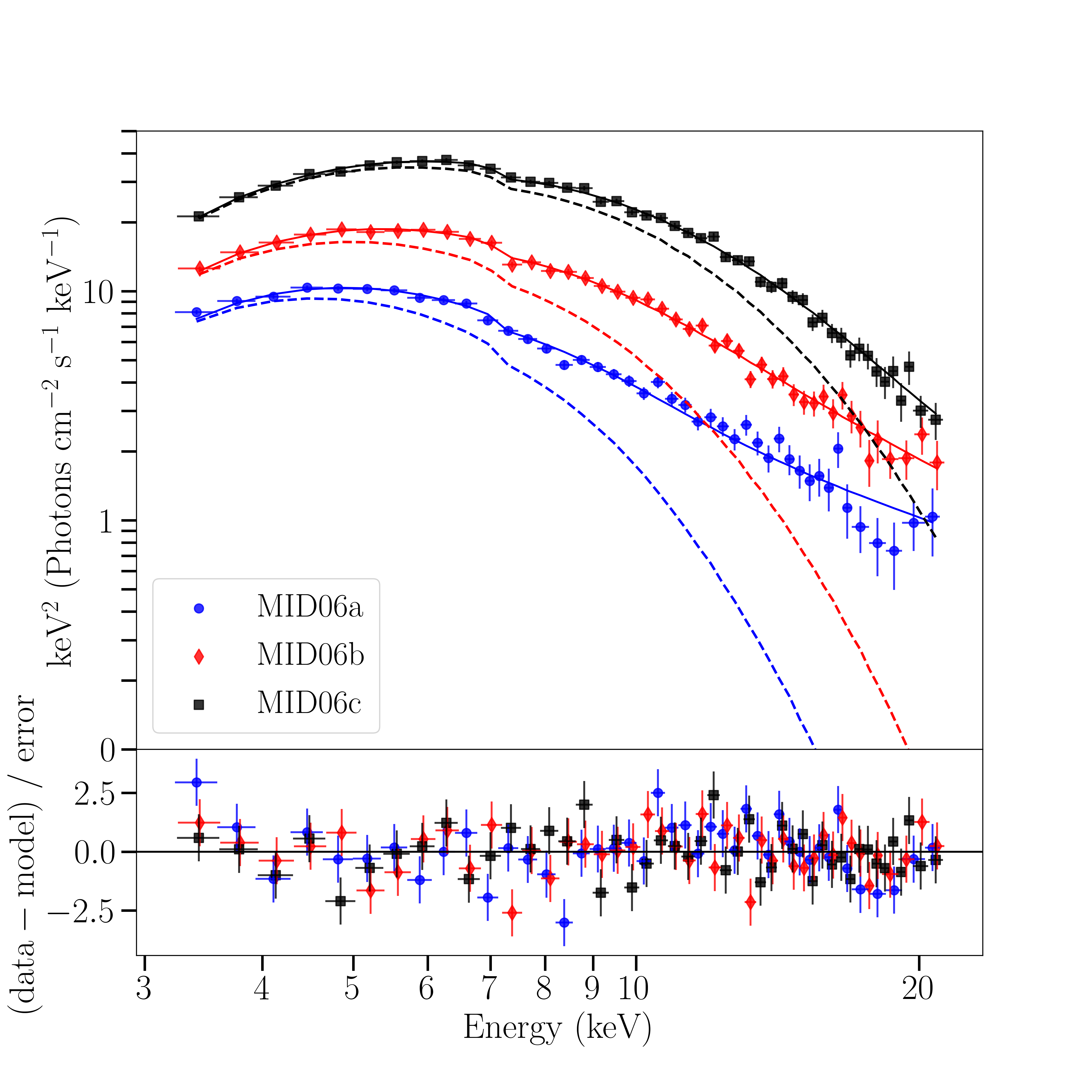
Figure 1: The top panel shows the three MID06 RXTE observations, MID06a (blue circles), MID06b (red diamonds), and MID06c (black squares), tied together and fit with the model mid:bhspec+simpl. The mass, distance, and inclination in bhspec were fixed to the R14 preferred values for the GRS 1915+105 system ($M=12.4$ $M_{\odot}$, $D=8.6$ kpc, and $i=60$°). The solid lines show the total model fit for each observation, and the dashed lines show the disk contribution for each spectral fit by setting the simpl scattering fraction to zero. The bottom panel shows the respective fit residuals.

In their analysis, MCC06 used a variation of bhspec and kerrbb which they call kerrbb2 to fit the soft X-ray continuum. This hybrid model includes the returning radiation and limb darkening capabilities from kerrbb while constraining the color correction factor, or spectral hardening factor, $f_{\rm{col}}$ using look-up tables generated from bhspec. They also used the Comptonization model comptt (Titarchuk, 1994) to fit the hard X-ray spectral component. To stay consistent in our re-analysis of the two papers, we chose to use simpl for the MCC06 data as we did for the MID06 data. We first fit MCC06a, MCC06b, and MCC06c tied together using only phabs, bhspec, and simpl, fixing the mass, distance, and inclination to the values previously assumed by MCC06 ($M=14$ $M_{\odot}$, $D=11$ kpc, and $i=66$°). We were unable to obtain a reasonable fit, with $\chi_{\nu}^{2}$ $=4090.6/150$. We then added the smedge and gaussian components, along with an addition absorption edge component, edge, which MCC06 used to improve their fit results. Here we adopt the same edge prescription, fixing the energy to lie between $8.0-13.0$ keV. We also kept the same abundance and parameter constraints as outlined in Section 3.1, and label this model mcc:bhspec+simpl. Adding these components significantly improved the fit results with $\chi_{\nu}^{2}$ $=139.4/132$ and provided a similar spin ($a_{*}\sim 0.977$) when compared to the spin reported by MCC06 ($a_{*}\gtrsim 0.98$). Keeping these model components in our fit, we then fixed the mass, distance, and inclination to the R14 preferred values, but were unable to get a good fit with $\chi_{\nu}^{2}$ $=835.5/132$ and the $a_{*}$ became pegged at the maximum spin allowed by bhspec ($a_{*}=0.99$).

In contrast to bhspec, the relativistic accretion disk model kerrbb allows the color correction factor $f_{\rm{col}}$ to vary as a free parameter. However, fitting for $a_{*}$ while allowing $f_{\rm{col}}$ to be free did not give reliable spin estimates, as the two parameters share a strong degeneracy (Salvesen & Miller, 2020). We discuss fitting kerrbb to the selected MCC06 observations fixing $f_{\rm{col}}$ at different values in the next section.

3.3 Color correction factor

We fit MCC06a, MCC06b, and MCC06c tied together and fit with the model mcc:kerrbb+simpl. The same parameter restrictions for the edge, smedge, and gaussian components discussed in Section 3.2 were again used in this model. For the kerrbb parameters, we assumed zero torque at the inner boundary, limb-darkening, and self-irradiation. The mass, distance, and inclination were fixed at the R14 preferred values. We then fixed $f_{\rm{col}}$ at different values ranging between $1.4-3.1$ and show each resulting best-fit $a_{*}$ and $\chi_{\nu}^{2}$ (126 degrees of freedom) plotted as black dots in Figure 2. Over-plotted in the figure are two estimates of $f_{\rm{col}}$ obtained by fitting kerrbb to bhspec: one for fixed $L/L_{\mathrm{Edd}}=0.1$ (shown as blue diamonds), and one for fixed $L/L_{\mathrm{Edd}}=1$ (shown as red X’s). A reasonable fit can be obtained for color correction factors $f_{\rm{col}}$ $\gtrsim 1.7$ if $a_{*}=0.999$. Lower spins only provide acceptable fits with higher values of $f_{\rm{col}}$, but sufficiently high values of $f_{\rm{col}}$ only occur for $L/L_{\rm{Edd}}$ greater than inferred for the MCC06 data. A representative best-fit to the three spectra by arbitrarily fixing $f_{\rm{col}}$ $=2.0$ is shown in Figure 3 where the best-fit spin is $a_{*}=0.995^{+0.002}_{-0.003}$ and $\chi_{\nu}^{2}$$=77.6/126$.

Figure 2: Plot showing the range of color correction factor values $f_{\rm{col}}$ for the three chosen MCC06 observations MCC06a, MCC06b, MCC06c tied together and fit with the mcc:kerrbb+simpl model, shown as black dots. The corresponding best-fit dimensionless spin parameter $a_{*}$ is shown in the top panel, and $\chi_{\nu}^{2}$ (126 degrees of freedom) is shown in the bottom panel. These fits were calculated assuming a mass, distance, and inclination fixed at the R14 preferred values ($M=12.4$ $M_{\odot}$, $D=8.6$ kpc, and $i=60$°). Estimates for $f_{\rm{col}}$, found by fitting kerrbb to bhspec are overplotted for a fixed $L/L_{\mathrm{Edd}}=0.1$ (blue diamonds) and a fixed $L/L_{\mathrm{Edd}}=1$ (red X’s). The horizontal line in the bottom panel shows $\chi_{\nu}^{2}$ $=1$ for reference.

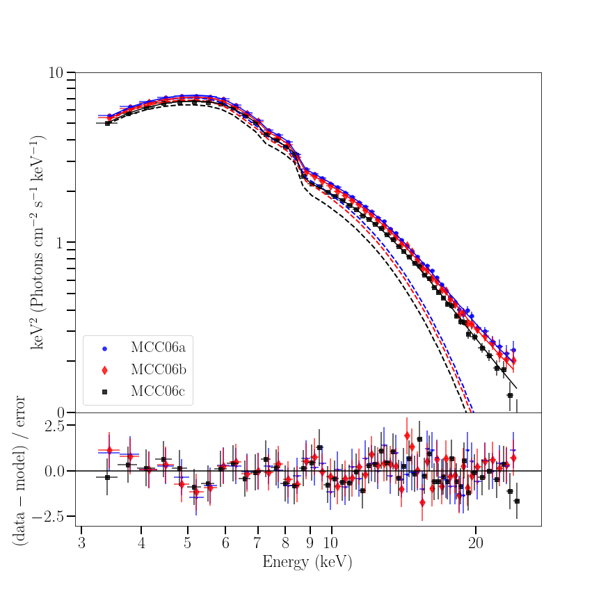
Figure 3: The top panel shows the three MCC06 RXTE observations MCC06a, MCC06b, MCC06c tied together and fit with the model mcc:kerrbb+simpl. The mass, distance, and inclination were fixed at the R14 preferred values for GRS 1915+105 ($M=12.4$ $M_{\odot}$, $D=8.6$ kpc, and $i=60$°). The kerrbb color correction factor, or spectral hardening factor, was arbitrarily fixed at $f_{\rm{col}}$ $=2.0$. The dashed lines show the contribution of the disk emission for each spectral fit by setting the simpl scattering fraction to zero. The bottom panel shows the fit residuals for each spectrum.

3.4 Exploring System Uncertainties

The uncertainty on the best-fit spin depends directly on the uncertainties in the distance, mass, and inclination. We explored this uncertainty in parameter space by fixing the mass, distance, and inclination at a range of different values above and below the R14 preferred values. A distance was randomly sampled from a Gaussian distribution centered on 8.6 kpc, with a 2.0 kpc width chosen to approximately match their uncertainty. From R14, the dependence of the inclination on a given distance is constrained from VLBI proper motion constraints, assuming ballistic trajectories for the plasma emitting in the jet. This gives

$$\tan{i}=\left(\frac{2D}{c}\right)\left(\frac{\mu_{\mathrm{a}}\mu_{\mathrm{r}}}{\mu_{\mathrm{a}}-\mu_{\mathrm{r}}}\right),$$ (1)

where $i$ is the inclination of the accretion disk with respect to the line of sight ($i=0$ is a face-on disk), $D$ is the distance to the black hole, $\mu_{a}$ is the apparent speed of the approaching radio jet, and $\mu_{r}$ is the apparent speed of the receding radio jet. The values for $\mu_{a}$ and $\mu_{r}$ were also sampled from Gaussian distributions centered on their reported values of 23.6 $\pm$ 0.5 milliarcseconds/yr and 10.0 $\pm$ 0.5 milliarcseconds/yr, respectively (R14). The mass of the black hole is then determined by using the inclination from equation (1) in the following expression:

$$M=\frac{\mathcal{M}}{\sin^{3}{i}},$$ (2)

where $M$ is the black hole mass, and $\mathcal{M}$ is a constant adopted from the values for the mass function and binary mass ratio in Steeghs et al. (2013). For each fit, the randomly selected distance and subsequent inclination and mass were held fixed while the three MID06 observations were simultaneously fit with the model mid:bhspec+simpl. The results from each fit are plotted in Figure 4 which shows the spread in parameter space for mass, distance, and inclination, as well as a histogram of all best-fit $a_{*}$ obtained. The black dots are fits which are within 99% confidence, $\chi_{\nu}^{2}$ $\leq 164.7/125$, and the red dots are fits with $\chi_{\nu}^{2}$ $>164.7/125$ which highlight regions where fits either became pegged at the maximum spin or the maximum luminosity limit of bhspec. The pile-up of fits at high spin have pegged at the maximum spin limit of bhspec ($a_{*}=0.99$), and fits below $a_{*}\sim 0.5$ signify observation MID06c has pegged at the luminosity limit of bhspec ($L/L_{\mathrm{Edd}}=1.77$). The R14 preferred values are marked as magenta X’s at the best-fit spin, $a_{*}=0.86$, for the MID06 observations. The previously assumed values for the mass, distance, and inclination from MID06 are marked as black X’s. The bottom x-axis is the logarithm of ($1-a_{*}$) to better show the portion of moderate to maximal spins, while the top x-axis is just $a_{*}$.

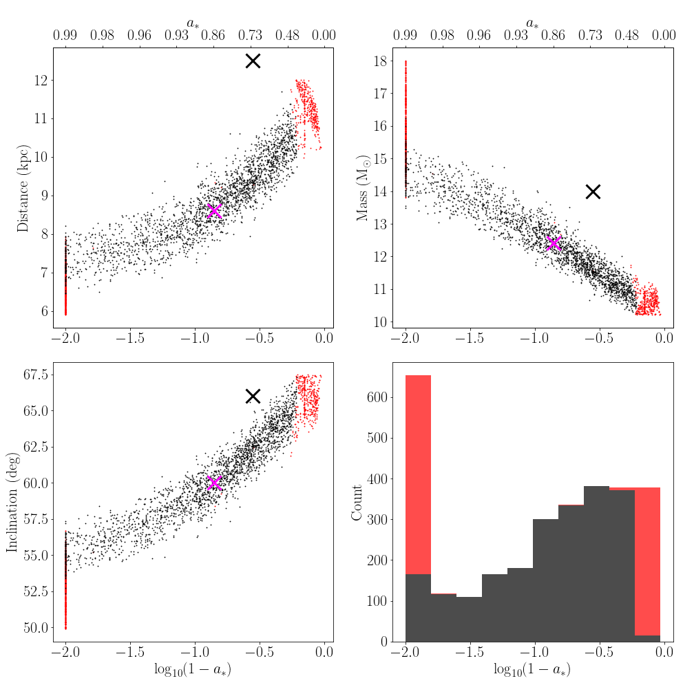
Figure 4: Range of parameter space for the mass, distance, inclination, and resulting best-fit spin, $a_{*}$, for fits to the three MID06 observations, MID06a, MID06b, MID06c tied together and fit with the model mid:bhspec+simpl (see Section 3.2). These fits account for the parameter dependence of inclination and mass on the distance to GRS 1915+105 via equations (1) and (2) (R14). Each distance was randomly sampled from a Gaussian distribution centered on the R14 preferred value $D=8.6$ kpc. The black dots indicate fits with $\chi_{\nu}^{2}$ $\leq 164.7/125$ which are within 99% confidence. The red dots in each panel indicate fits with $\chi_{\nu}^{2}$ $>164.7/125$ which are outside the 99% confidence. The pile-up of red dots at high spins is due to fits which have pegged at the maximum spin limit of bhspec ($a_{*}=0.99$). The red fits at lower spins $a_{*}\lesssim 0.5$ indicate fits in which observation MID06c has pegged at the luminosity limit of bhspec ($L/L_{\mathrm{Edd}}=1.77$, where $L_{\mathrm{Edd}}$ is the Eddington luminosity). The bottom right panel shows a histogram of all the resulting best-fit spins obtained for the MID06 observations. The R14 preferred values ($D=8.6$ kpc, $M=12.4$ $M_{\odot}$, $i=60$°) are marked with a magenta colored “X” at the best-fit spin for these assumed values, $a_{*}=0.863^{+0.014}_{-0.015}$. The best-fit parameter values are listed in Table 2 for the R14 preferred values). The distance, mass, and inclination previously assumed by MID06 (12.5 kpc, 14 $M_{\odot}$, 66°, respectively) are marked with a black “X” for comparison.

The same random sampling continuum-fitting analysis was done for the three MCC06 observations, the results of which are shown in Figure 5. This plot shows the range of distances, masses, and inclinations which produce fits to this dataset within 99% confidence ($\chi_{\nu}^{2}$ $<172.66/132$) using the model mcc:bhspec+simpl and the same parameter prescription in Section 3.2. Each dot is one realization for a fixed mass, distance, and inclination, color-coded by the best-fit spin as shown by the color bar.

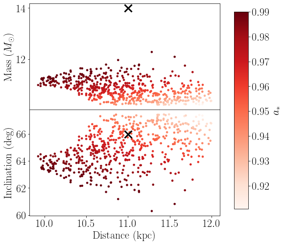
Figure 5: Range of parameter space for the mass, distance, and inclination for the three MCC06 observations MCC06a, MCC06b, MCC06c, simultaneously fit together with the model mcc:bhspec+simpl. Each dot represents one realization for a given fixed mass, distance, and inclination, the resulting spin of which is shown by the color bar. All fits shown here are within 99% confidence ($\chi_{\nu}^{2}$ $\leq 172.7/132$). The black X’s mark the system parameter values previously assumed by MCC06 ($M=14$ $M_{\odot}$, $D=11$ kpc, and $i=66$°), whereas the new R14 values are not within range.

4 Discussion

4.1 Implications for the GRS 1915+105 system

The relative merits of the MCC06 and MID06 data selection were debated in those papers and are summarized in Section 1. We will not discuss this at further length here but we note that one of the objections to the MID06 datasets is that their larger Eddington ratios imply thicker accretion disks, potentially invalidating the assumptions of the thin disk model underlying the bhspec model. With the revised system parameters, the implied Eddington ratios are now slightly lower, with the lowest Eddington observation being in a range where the disk model remains relatively thin. More generally, the relatively high Eddington ratio of GRS 1915+105 is sometimes hypothesized to account for its relatively unique variability, but our best-fit constraints imply the source is generally sub-Eddington or at most slightly super-Eddington.

Although more moderate spins are allowed by the MID06 datasets, relatively high spin is implied for the R14 best-fit system parameters. Black holes in X-ray binaries are expected to be born with low to moderate spins ($a_{*}\lesssim 0.7$), although this is subject to uncertainties in the core-collapse process (Gammie et al., 2004). It is also not clear that they can be significantly spun up by accretion under standard assumptions about mass transfer (King & Kolb, 1999). The high spins inferred here would then imply that either black holes are born with higher natal spin than expected or experience phases of high mass transfer to spin them up.

It is perhaps notable that the best-fit values from MID06 are in the ballpark where general relativistic magnetohydrodynamic simulations suggest magnetic torques would balance the spin-up due to accretion (Gammie et al., 2004). This limit ($a_{*}\lesssim 0.94$) is more stringent than the commonly cited limit of $a_{*}=0.998$ from Thorne (1974), which only accounts for the angular momentum carried by the radiated photons. The MID06 results are thus consistent with GRS 1915+105 being spun up by accretion and reaching an equilibrium with magnetohydrodynamic torques provided by field lines connected to the black hole, while MCC06 results exceed this nominal limit. Note, however, that the presence of such torques may have an effect on the accretion disk emission (Gammie, 1999; Agol & Krolik, 2000; Kulkarni et al., 2011; Schnittman et al., 2016) and are not accounted for in the present analysis.

Our results for the MID06 data are inconsistent with those of R14, who report best-fit $a_{*}\simeq 0.98$. Accounting for systematic uncertainties, they report $a_{*}>0.92$, which is consistent with our lower limit from Figure 5. Our results for the MCC06 data are in better agreement in that both analyses favor near maximal spin but differ in that R14 managed to find suitable fits for the revised distance of $8.6$ kpc. This may owe in part to R14 reanalyzing a large sample of RXTE observations, selecting all observations that obey a criterion $L/L_{\rm Edd}\leq 0.3$, $\chi^{2}_{\nu}\leq 2$, and $f_{\rm sc}<0.25$. It is possible that the MCC06 selected datasets may have been selected out in the process using the revised system parameters. Sreehari et al. (2020) also find a near maximal best-fit spin for kerrbb fits to AstroSat observations of GRS 1915+105. These results are notable in that, like MID06, they are for observations that would nominally place the emission above the Eddington limit. Their analysis differs in allowing the mass to be a free parameter, although their best-fit mass is consistent with the R14 constraints.

In addition to the continuum-fitting method, the spin of GRS 1915+105 has also been estimated by fitting the relativistically broadened reflection spectrum due to irradiation of the accretion disk by a corona (Blum et al., 2009; Miller et al., 2013) or via modeling of quasiperiodic oscillations (QPOs; Török et al., 2011; Šrámková et al., 2015). Although a range of results have been reported with both methods, the reflection fitting efforts are both consistent with high spins $a_{*}\simeq 0.98$ while the QPO model favors somewhat lower spins $a_{*}\sim 0.7-0.9$. Based on previous results, this puts the reflection fitting results in good agreement with MCC06 and the QPO estimates in better agreement with MID06. For our results, the MCC06 fits are still broadly in agreement with near maximal spin as long as GRS 1915+105 lies at the far end of the distance distribution allowed by VLBI parallax. The MID06 data now provide a larger best-fit spin in better agreement with reflection fitting. More moderate spins are still favored albeit with large uncertainty.

4.2 Impact and Uncertainties in Interstellar Absorption

Typically when fitting the continuum of a BHXRB, a model for the photoelectric absorption along the line of sight (e.g. phabs, varabs) is needed. Using the model varabs and abundances from Anders & Ebihara (1982), MID06 assumed a column value of $n_{\rm{H}}=4.7\times 10^{22}$ $\rm{cm}^{-2}$ for all elements except Si and Fe which were fixed at $16.4\times 10^{22}$ $\mathrm{cm^{-2}}$ and $10.9\times 10^{22}$ $\mathrm{cm^{-2}}$, respectively. These values were reported by Lee et al. (2002) for Chandra X-ray observations of GRS 1915+105 assuming ISM abundances. Relativistic disk reflection studies constraining the spin in GRS 1915+105 report best-fit values which also favor a high absorption column using the phabs model ($n_{\rm{H}}=4.15-5.64\times 10^{22}$ $\rm{cm}^{-2}$, Blum et al. 2009; $n_{\rm{H}}=6.1\times 10^{22}$ $\rm{cm}^{-2}$, Miller et al. 2013). Lee et al. (2002) also reported a S- and Mg-derived hydrogen column assuming solar abundances, giving a more moderate column value of $n_{\rm{H}}\sim 3.1\times 10^{22}$ $\rm{cm}^{-2}$. This is in better agreement with other modest column estimates from ASCA X-ray observations ($n_{\rm{H}}=3.8\times 10^{22}$ $\rm{cm}^{-2}$, Ebisawa et al., 1994) along with millimeter and radio observations ($n_{\rm{H}}=3.6\times 10^{22}$ $\rm{cm}^{-2}$, Chapuis & Corbel, 2004). Following these modest estimates, MCC06 adopted a value of $n_{\rm{H}}=4.0\times 10^{22}$ $\rm{cm}^{-2}$ (assuming abundances from Anders & Grevesse 1989).

Not only did MCC06 and MID06 assume different values for the column, they also chose different XSPEC absorption models. MCC06 selected phabs for their analysis, while MID06 chose varabs. We found that when using the same $n_{\rm{H}}$ value and all other variables kept the same, varabs tended toward a lower $a_{*}$ than phabs did. Fits to the MCC06 data with either phabs or varabs tended to fit better with low $n_{\rm{H}}$ values, while fits to the MID06 data tended to fit better with higher $n_{\rm{H}}$ values. An overall trend between both varabs and phabs is that the value for $a_{*}$ decreased as the $n_{\rm{H}}$ column increased for both datasets. To maintain consistency in our re-analysis we kept the same XSPEC absorption models and values for $n_{\rm{H}}$ chosen by each group, but note the sensitivity and dependence of the spin on the assumed $n_{\rm{H}}$ column value as a source of uncertainty in the $a_{*}$ estimate in this work.

Aside from the line-of-sight hydrogen column estimates, kinematic studies near GRS 1915+105 have also located a molecular cloud at a distance of $9.4\pm 0.2$ kpc (Chaty et al., 1996; Chapuis & Corbel, 2004). The new VLBI constraints may have implications for the history and conception of the GRS 1915+105 system given the distance of $8.6$ kpc, which could place it with the observed interstellar structure (R14).

4.3 Uncertainties in Spin, Models, and System Parameters

The R14 VLBI parallax measurements provide much stronger constraints on the system parameters than were previously available, but our analysis shows that remaining uncertainties still allow for a rather large range of spins. If we treat the models as robust to systematic uncertainties, then our fitting constraints nominally imply strict limits on the system parameters. Figure 4 implies that for relatively low distances and inclinations, the implied spin from the MID06 data would be higher than $a_{*}=0.99$, challenging the theoretical understanding on black hole spin limits. The constraints are even stronger for the MCC06 data, which would limit the distances to $D\gtrsim 10$ kpc, near the outer limits of what is allowed by the R14 constraints. In fact, this result is consistent with predictions made in Figure 18 of MCC06, which predicted GRS 1915+105 to lie within an error triangle whose minimum distance was just under $\sim 10$ kpc.

The model for system parameters implied by equations (1) and (2) is also subject to systematic uncertainties. First, equation (1) assumes the observed superluminal motion can be interpreted as emission from plasma following ballistic trajectories and that these trajectories lie along the spin axis of the black hole. Furthermore, it is conceivable that the plane of the binary is not perpendicular to the black hole spin axis (Fragile et al., 2001; Maccarone, 2002), although there are theoretical arguments that such misalignments should typically be modest (Fragos & McClintock, 2015). If such misalignment is present, it seems likely that the inner accretion disk would align with the spin axis due to the action of Lense-Thirring precession (Bardeen & Petterson, 1975). In this case, our use of the jet to fix the disk inclination would still be reasonable as long as the jet is aligned with the spin axis, although GRMHD simulations of misaligned disks indicate this may not be guaranteed (Liska et al., 2018) and observations of V404 Cygni show the jet angle to precess (Miller-Jones et al., 2019) perhaps due to Lense-Thirring precession associated with the high mass accretion rates inflating the disk (Middleton et al., 2018, 2019). The inclination implied by observations of the jet would then not correspond to the binary inclination in equation (2), and the inferred black hole mass would be incorrect.

An independent constraint on the inclination comes from the reflection spectral modeling, where the relativistic line profiles are sensitive to the viewing inclination. The best-fit inclinations from Blum et al. (2009) are $i=55^{\circ}$ or $i=69^{\circ}$ depending on the reflection model used. Miller et al. (2013) found inclinations ranging from $65^{\circ}$ to $74^{\circ}$ depending on the model. Blum et al. (2009) constrained the inclination to lie between $55^{\circ}$ and $75^{\circ}$, while Miller et al. (2013) constrained it to be between $65^{\circ}$ and $80^{\circ}$, both based on interpretations of constraints from the superluminal jet model (Fender et al., 1999). The allowed inclination ranges are generally higher than those used in our analysis because these papers predate the R14 measurements. The higher inclinations ($i\gtrsim 70^{\circ}$) would pose a challenge to the super-luminal motion interpretation for the new parallax distance, but if we assume they imply that the inclination should be towards the high end of the allowed range, they would push the MID06 results to low spins that would be at odds with the best-fit spins from these reflection models. The MCC06 results could remain consistent with near maximal spin, but again this requires GRS 1915+105 to be located at the more distant end of the range allowed by VLBI parallax measurements.

Finally, we emphasize that these constraints are subject to unquantified systematic uncertainties in the underlying accretion disk model. This could arise from inaccuracies in the underlying thin disk model (Shakura & Sunyaev, 1973; Novikov & Thorne, 1973) or because of errors in the TLUSTY atmosphere models (Davis & Hubeny, 2006). The former is perhaps most worrisome for the highest Eddington ratio observations from MID06, where the thin disk assumption would begin to break down. It is also possible that some aspect of the model is inaccurate, such as the stress prescription (Done & Davis, 2008), assumption of a torque-free inner boundary (Gammie, 1999; Agol & Krolik, 2000) and truncation of emission at the ISCO (Krolik & Hawley, 2002; Abramowicz et al., 2010). The relativistic thin disk models employed here are broadly consistent with GRMHD models, but emission interior to the ISCO and magnetic torques would provide a modest bias towards higher spins when using standard models (Kulkarni et al., 2011; Schnittman et al., 2016). In that case, the near maximal best-fit spins might still be indicative of high spin, but not necessarily maximal spin. These models also assume a razor thin disk even though they can be at accretion rates where the thin disk assumption breaks down. Zhou et al. (2020) found that considering a model with a finite disk thickness led to a modestly higher spin for fits to RXTE observations of GRS 1915+105, but their thin disk fits were already near maximal.

The spectra derived from atmosphere modelling with TLUSTY are another potential source of error. Errors in the atmosphere models and spectra could arise from inaccurate assumptions about the vertical distribution of dissipation, contributions from magnetic pressure support, inhomogeneities in the turbulent disk, and lack of irradiation of the surface (Davis et al., 2005; Blaes et al., 2006; Davis et al., 2009; Tao & Blaes, 2013; Narayan et al., 2016). Figure 2 provides a sense of the degree to which spectral hardening errors would impact our spin results. Further discussion of the spectral hardening implied by TLUSTY calculations can be found in Davis & El-Abd (2019) while Salvesen & Miller (2021) provide a thorough review of uncertainties and quantitative estimates of their impact on spin measurements.

5 Summary and Conclusions

We re-examine the continuum-fitting based spin estimates for GRS 1915+105 in light of new constraints on the mass, distance, and inclination from VLBI parallax (R14). We find that the discrepancies between data selected by MID06 and MCC06 persist, implying that the selection criteria of one (or both) is inconsistent with the assumptions of the thin disk model. MCC06 showed a trend towards lower spin as the luminosity of the observations increased, indicating the discrepancy may be driven primarily by different Eddington ratio ranges of the two datasets. The revised system parameters lower the mass, but lead to relatively smaller implied luminosities, leading to lower overall Eddington ratios for fits to both datasets. This somewhat mitigates concerns that the Eddington ratios in the MID06 models were too high, but the highest Eddington ratio is still close to unity ($L/L_{\rm Edd}=0.87$), where the scale height of the disk is unlikely to remain small compared to the radius, as assumed in the model.

The new system parameters drive both datasets to higher spins. Since MCC06 were already fitting for near maximal spin, this presents a challenge. For the bhspec model (or kerrbb model with color corrections set to match bhspec), we cannot obtain a good fit for the preferred (R14) system parameters. Good fits to these data can only be found if the color correction is allowed to vary to values significantly higher ($f\gtrsim 2.2$) than implied by bhspec or the distance to GRS 1915+105 is near or greater than 10 kpc, consistent with the prediction of MCC06 (their Figure 18). The spin would remain near maximal ($a_{*}\simeq 0.99$) for a distance of 10 kpc, consistent with constraints from modeling of the reflection spectrum.

For the MID06 data, the best-fit spin is moderately high ($a_{*}\simeq 0.86$) for the best-fit R14 system parameters. We find, however, that a fairly broad range of spins are allowed when the uncertainty in the parallax distance and jet model inclination are accounted for, as indicated by Figure 4. In principle, this allows the spin to match constraints from either the near maximal spins from reflection modeling or the more moderate spins from QPO models. Near maximal spin, however, would result for fairly low inclinations in our model, which would be inconsistent with the best-fit inclinations from reflection modelling. The low end of the allowed spin distribution is sensitive to the maximum Eddington ratio permitted by bhspec ($L/L_{\rm Edd}=1.77$). Therefore, the lower limit on $a_{*}$ is tied to the Eddington ratio beyond which one says the thin disk model is no longer valid.

Although the VLBI parallax measurements are an impressive achievement, our results indicate that even stronger constraints are necessary to provide a tight constraint on the spin with the continuum-fitting method, and to help resolve the discrepancies driven by data selection. We note that such constraints also have implications for the reflection spectrum modeling through the dependence of relativistic Doppler shift and beaming on the observer inclination. This analysis would also benefit from better constraints on the interstellar absorption toward GRS 1915+105. The datasets modeled here prefer different models for the absorption and are particularly sensitive to the hydrogen column assumed. The range of columns used in the literature vary by more than a factor of two, which is enough to modify the best-fit spin, with larger assumed columns generally providing lower spins.

References

- Abramowicz et al. (2010) Abramowicz, M. A., Jaroszyński, M., Kato, S., et al. 2010, A&A, 521, A15, doi: 10.1051/0004-6361/201014467
- Agol & Krolik (2000) Agol, E., & Krolik, J. H. 2000, ApJ, 528, 161, doi: 10.1086/308177
- Altamirano et al. (2011) Altamirano, D., Belloni, T., Linares, M., et al. 2011, The Astrophysical Journal, 742, L17, doi: 10.1088/2041-8205/742/2/l17
- Anders & Ebihara (1982) Anders, E., & Ebihara, M. 1982, Geochim. Cosmochim. Acta, 46, 2363, doi: 10.1016/0016-7037(82)90208-3
- Anders & Grevesse (1989) Anders, E., & Grevesse, N. 1989, Geochim. Cosmochim. Acta, 53, 197, doi: 10.1016/0016-7037(89)90286-X
- Arnaud (1996) Arnaud, K. A. 1996, in Astronomical Society of the Pacific Conference Series, Vol. 101, Astronomical Data Analysis Software and Systems V, ed. G. H. Jacoby & J. Barnes, 17
- Bardeen & Petterson (1975) Bardeen, J. M., & Petterson, J. A. 1975, ApJ, 195, L65, doi: 10.1086/181711
- Belloni et al. (2000) Belloni, T., Klein-Wolt, M., Méndez, M., van der Klis, M., & van Paradijs, J. 2000, A&A, 355, 271. https://arxiv.org/abs/astro-ph/0001103
- Blaes et al. (2006) Blaes, O. M., Davis, S. W., Hirose, S., Krolik, J. H., & Stone, J. M. 2006, ApJ, 645, 1402, doi: 10.1086/503741
- Blum et al. (2009) Blum, J. L., Miller, J. M., Fabian, A. C., et al. 2009, ApJ, 706, 60, doi: 10.1088/0004-637X/706/1/60
- Chapuis & Corbel (2004) Chapuis, C., & Corbel, S. 2004, A&A, 414, 659, doi: 10.1051/0004-6361:20034028
- Chaty et al. (1996) Chaty, S., Mirabel, I. F., Duc, P. A., Wink, J. E., & Rodriguez, L. F. 1996, A&A, 310, 825. https://arxiv.org/abs/astro-ph/9612244
- Davis et al. (2009) Davis, S. W., Blaes, O. M., Hirose, S., & Krolik, J. H. 2009, ApJ, 703, 569, doi: 10.1088/0004-637X/703/1/569
- Davis et al. (2005) Davis, S. W., Blaes, O. M., Hubeny, I., & Turner, N. J. 2005, ApJ, 621, 372, doi: 10.1086/427278
- Davis & El-Abd (2019) Davis, S. W., & El-Abd, S. 2019, The Astrophysical Journal, 874, 23, doi: 10.3847/1538-4357/ab05c5
- Davis & Hubeny (2006) Davis, S. W., & Hubeny, I. 2006, ApJS, 164, 530, doi: 10.1086/503549
- Done & Davis (2008) Done, C., & Davis, S. W. 2008, ApJ, 683, 389, doi: 10.1086/589647
- Done et al. (2007) Done, C., Gierliński, M., & Kubota, A. 2007, A&A Rev., 15, 1, doi: 10.1007/s00159-007-0006-1
- Ebisawa (1991) Ebisawa, K. 1991, PhD thesis, Insititute of Space and Astronautical Science/Japan Aerospace Exploration Agency
- Ebisawa et al. (1994) Ebisawa, K., Ogawa, M., Aoki, T., et al. 1994, PASJ, 46, 375
- Fabian et al. (1989) Fabian, A. C., Rees, M. J., Stella, L., & White, N. E. 1989, MNRAS, 238, 729, doi: 10.1093/mnras/238.3.729
- Fender et al. (1999) Fender, R. P., Garrington, S. T., McKay, D. J., et al. 1999, MNRAS, 304, 865, doi: 10.1046/j.1365-8711.1999.02364.x
- Fragile et al. (2001) Fragile, P. C., Mathews, G. J., & Wilson, J. R. 2001, ApJ, 553, 955, doi: 10.1086/320990
- Fragos & McClintock (2015) Fragos, T., & McClintock, J. E. 2015, ApJ, 800, 17, doi: 10.1088/0004-637X/800/1/17
- Gammie (1999) Gammie, C. F. 1999, ApJ, 522, L57, doi: 10.1086/312207
- Gammie et al. (2004) Gammie, C. F., Shapiro, S. L., & McKinney, J. C. 2004, ApJ, 602, 312, doi: 10.1086/380996
- Gierliński & Done (2004) Gierliński, M., & Done, C. 2004, MNRAS, 347, 885, doi: 10.1111/j.1365-2966.2004.07266.x
- Gierliński et al. (1999) Gierliński, M., Zdziarski, A. A., Poutanen, J., et al. 1999, MNRAS, 309, 496, doi: 10.1046/j.1365-8711.1999.02875.x
- Hanawa (1989) Hanawa, T. 1989, ApJ, 341, 948, doi: 10.1086/167553
- King & Kolb (1999) King, A. R., & Kolb, U. 1999, MNRAS, 305, 654, doi: 10.1046/j.1365-8711.1999.02482.x
- Krolik & Hawley (2002) Krolik, J. H., & Hawley, J. F. 2002, ApJ, 573, 754, doi: 10.1086/340760
- Kulkarni et al. (2011) Kulkarni, A. K., Penna, R. F., Shcherbakov, R. V., et al. 2011, MNRAS, 414, 1183, doi: 10.1111/j.1365-2966.2011.18446.x
- Lee et al. (2002) Lee, J. C., Reynolds, C. S., Remillard, R., et al. 2002, ApJ, 567, 1102, doi: 10.1086/338588
- Li et al. (2005) Li, L.-X., Zimmerman, E. R., Narayan, R., & McClintock, J. E. 2005, ApJS, 157, 335, doi: 10.1086/428089
- Liska et al. (2018) Liska, M., Hesp, C., Tchekhovskoy, A., et al. 2018, MNRAS, 474, L81, doi: 10.1093/mnrasl/slx174
- Maccarone (2002) Maccarone, T. J. 2002, MNRAS, 336, 1371, doi: 10.1046/j.1365-8711.2002.05876.x
- McClintock et al. (2006) McClintock, J. E., Shafee, R., Narayan, R., et al. 2006, ApJ, 652, 518, doi: 10.1086/508457
- McClintock et al. (2011) McClintock, J. E., Narayan, R., Davis, S. W., et al. 2011, Classical and Quantum Gravity, 28, 114009, doi: 10.1088/0264-9381/28/11/114009
- Middleton (2016) Middleton, M. 2016, Astrophysics and Space Science Library, 99–151, doi: 10.1007/978-3-662-52859-4_3
- Middleton et al. (2006) Middleton, M., Done, C., Gierliński, M., & Davis, S. W. 2006, MNRAS, 373, 1004, doi: 10.1111/j.1365-2966.2006.11077.x
- Middleton et al. (2019) Middleton, M. J., Fragile, P. C., Ingram, A., & Roberts, T. P. 2019, MNRAS, 489, 282, doi: 10.1093/mnras/stz2005
- Middleton et al. (2018) Middleton, M. J., Fragile, P. C., Bachetti, M., et al. 2018, MNRAS, 475, 154, doi: 10.1093/mnras/stx2986
- Miller et al. (2013) Miller, J. M., Parker, M. L., Fuerst, F., et al. 2013, ApJ, 775, L45, doi: 10.1088/2041-8205/775/2/L45
- Miller-Jones et al. (2019) Miller-Jones, J. C. A., Tetarenko, A. J., Sivakoff, G. R., et al. 2019, Nature, 569, 374, doi: 10.1038/s41586-019-1152-0
- Mitsuda et al. (1984) Mitsuda, K., Inoue, H., Koyama, K., et al. 1984, PASJ, 36, 741
- Narayan et al. (2016) Narayan, R., Zhu, Y., Psaltis, D., & Sadowski, A. 2016, MNRAS, 457, 608, doi: 10.1093/mnras/stv2979
- Novikov & Thorne (1973) Novikov, I. D., & Thorne, K. S. 1973, in Black Holes (Les Astres Occlus), 343–450
- Reid et al. (2014) Reid, M. J., McClintock, J. E., Steiner, J. F., et al. 2014, ApJ, 796, 2, doi: 10.1088/0004-637X/796/1/2
- Remillard & McClintock (2006) Remillard, R. A., & McClintock, J. E. 2006, ARA&A, 44, 49, doi: 10.1146/annurev.astro.44.051905.092532
- Salvesen & Miller (2020) Salvesen, G., & Miller, J. M. 2020, MNRAS, doi: 10.1093/mnras/staa3325
- Salvesen & Miller (2021) —. 2021, MNRAS, 500, 3640, doi: 10.1093/mnras/staa3325
- Schnittman et al. (2016) Schnittman, J. D., Krolik, J. H., & Noble, S. C. 2016, ApJ, 819, 48, doi: 10.3847/0004-637X/819/1/48
- Shafee et al. (2006) Shafee, R., McClintock, J. E., Narayan, R., et al. 2006, ApJ, 636, L113, doi: 10.1086/498938
- Shakura & Sunyaev (1973) Shakura, N. I., & Sunyaev, R. A. 1973, A&A, 500, 33
- Sreehari et al. (2020) Sreehari, H., Nandi, A., Das, S., et al. 2020, MNRAS, 499, 5891, doi: 10.1093/mnras/staa3135
- Steeghs et al. (2013) Steeghs, D., McClintock, J. E., Parsons, S. G., et al. 2013, ApJ, 768, 185, doi: 10.1088/0004-637X/768/2/185
- Steiner et al. (2009) Steiner, J. F., Narayan, R., McClintock, J. E., & Ebisawa, K. 2009, PASP, 121, 1279, doi: 10.1086/648535
- Tao & Blaes (2013) Tao, T., & Blaes, O. 2013, ApJ, 770, 55, doi: 10.1088/0004-637X/770/1/55
- Thorne (1974) Thorne, K. S. 1974, ApJ, 191, 507, doi: 10.1086/152991
- Titarchuk (1994) Titarchuk, L. 1994, ApJ, 434, 570, doi: 10.1086/174760
- Török et al. (2011) Török, G., Kotrlová, A., Šrámková, E., & Stuchlík, Z. 2011, A&A, 531, A59, doi: 10.1051/0004-6361/201015549
- Šrámková et al. (2015) Šrámková, E., Török, G., Kotrlová, A., et al. 2015, A&A, 578, A90, doi: 10.1051/0004-6361/201425241
- Zdziarski et al. (2005) Zdziarski, A. A., Gierliński, M., Rao, A. R., Vadawale, S. V., & Mikołajewska, J. 2005, MNRAS, 360, 825, doi: 10.1111/j.1365-2966.2005.09112.x
- Zdziarski et al. (1996) Zdziarski, A. A., Johnson, W. N., & Magdziarz, P. 1996, MNRAS, 283, 193, doi: 10.1093/mnras/283.1.193
- Zhang et al. (1997) Zhang, S. N., Cui, W., & Chen, W. 1997, ApJ, 482, L155, doi: 10.1086/310705
- Zhou et al. (2020) Zhou, M., Abdikamalov, A. B., Ayzenberg, D., et al. 2020, MNRAS, 496, 497, doi: 10.1093/mnras/staa1591
- Życki et al. (1999) Życki, P. T., Done, C., & Smith, D. A. 1999, MNRAS, 309, 561, doi: 10.1046/j.1365-8711.1999.02885.x