Towards studying the structural differences between the pion and its radial excitation

Abstract

We present an exploratory lattice QCD investigation of the differences between the valence quark structure of pion and its radial excitation $\pi(1300)$ in a fixed finite volume using the leading-twist factorization approach. We present evidences that the first pion excitation in our lattice computation is a single particle state that is likely to be the finite volume realization of $\pi(1300)$. An analysis with reasonable priors result in better estimates of the excited state PDF and the moments, wherein we find evidence that the radial excitation of pion correlates with an almost two-fold increase in the momentum fraction of valence quarks. This proof-of-principle work establishes the viability of future lattice computations incorporating larger operator basis that can resolve the structural changes accompanying hadronic excitation.

I Introduction

The parton structure of pion has garnered both experimental Badier et al. (1983); Betev et al. (1985); Conway et al. (1989); Owens (1984); Sutton et al. (1992); Gluck et al. (1992, 1999); Wijesooriya et al. (2005); Barry et al. (2018); Novikov et al. (2020) as well as theoretical efforts Aicher et al. (2010); Nguyen et al. (2011); Chen et al. (2016a); Cui et al. (2020); Roberts and Schmidt (2020); de Teramond et al. (2018); Ruiz Arriola (2002); Broniowski and Ruiz Arriola (2017); Lan et al. (2020); Bednar et al. (2020). A better determination of the quark structure of pion is also part of the goals of upcoming experimental facilities Aguilar et al. (2019); Adams et al. (2018). In addition to experimental determinations, due to the recent breakthroughs in computing parton structure using the Euclidean lattice QCD simulations via leading-twist perturbative factorization approaches (Large Momentum Effective Theory Ji (2013, 2014), short-distance factorization of the pseudo distribution Radyushkin (2017a); Orginos et al. (2017), current-current correlators  Braun and Müller (2008); Ma and Qiu (2018a, b), which has also been dubbed as good lattice cross sections Ma and Qiu (2018b), and Refs Constantinou (2020); Zhao (2019); Cichy and Constantinou (2019); Monahan (2018); Ji et al. (2020a) for extensive reviews on the methodology), the valence quark structure of pion has also been investigated from first-principle QCD computations Gao et al. (2020); Zhang et al. (2019); Izubuchi et al. (2019); Joó et al. (2019); Lin et al. (2020); Sufian et al. (2019, 2020); Karthik (2021). The large-$x$ behavior of the valence pion PDF has been an unresolved issue that has been approached using all the above lines of attack, with the promise of being settled in the near future by lattice computations with finer lattices, realistic physical pion masses and with the usage of highly boosted pion states to reduce higher-twist effects that might be amplified Braun et al. (2019); Liu and Chen (2020); Ji et al. (2020b) near $x=1$.

The considerable interest in the quark structure of pion is due to its special role as the Nambu-Goldstone boson of chiral symmetry breaking in QCD. The grand goal of this research direction is to understand the aspects of mass-gap generation in QCD via the quark-gluon interaction within the pion. The large-$x$ behavior of pion PDF has been proposed to hold the key to make this connection (c.f., Roberts (2020)). While the enigmatic aspect of QCD is the presence of nonvanishing mass-gap between the vacuum and the ground-states of various quantum numbers even in the chiral limit (except the pseudo-scalar, which is an exception), it is equally enigmatic that there are non-zero mass-gaps amongst the excited states in the tower of excited spectrum as well. To contrast, if the trace-anomaly was absent in QCD, there would not be mass-gaps between the vacuum and the various ground-states, nor between the excited states. Given the stark dissimilarity between the vanishing mass of a pion in the chiral limit and the nonvanishing masses of its excited states in the same limit, it is reasonable to expect any differences between the quark and gluon structures of the ground-state pion and its excited states could help us understand the mechanism behind spontaneous symmetry-breaking and the mass-gap generation better. In this respect, there have been prior lattice computations to study the decay constants of the pion and its radial excitation McNeile and Michael (2006); Mastropas and Richards (2014), where the decay constant of the radial excitation is expected to vanish in the chiral limit unlike that of the ground-state pion Holl et al. (2004). Closely related to the decay constant, the distribution amplitudes of the pion and its radial excitation have also been previously studied using the Dyson-Schwinger Equation Li et al. (2016). With the lattice computation of PDFs now possible, a novel theoretical research direction to study not just the differences between the long-distance behaviors of the ground and the excited states, but to study the differences in their internal structural properties is promising. In this respect, we should also point to a previous study Chai et al. (2020) of the $\Delta^{+}$ baryon on the lattice, which differs by both mass and angular momentum from that of the proton. Since there is also experimental thrust to understand exotic gluon excitations of mesons in Jefferson Lab 12 GeV program Dudek et al. (2012), studies as the present one on the parton structure of simpler radial excitations, might be helpful phenomenologically by providing a case to contrast the exotic transitions with.

Figure 1: The dependence of the first-excited state energy $E_{1}(\mathbf{P})$ on the range $[t_{\rm min},32]$ used in the two-state fits to the SS correlator is shown. The different panels are for six different values of momentum $\mathbf{P}=(0,0,P_{z})$. For large $t_{\rm min}$, the best fit values have a tendency to approach the dispersion values, $E_{1}=\sqrt{P_{z}^{2}+M_{1}^{2}}$ with $M_{1}=1.5$ GeV, shown as the horizontal lines.

It is the aim of this paper to point to the possibility of studying the structural differences between the pion and its radial excitation Tanabashi et al. (2018), $\pi(1300)$. In this paper, we will provide reasonable evidences to justify that the excited state that we observe on the lattice shows properties of a single particle state with similar mass to that of $\pi(1300)$, a broad resonance state with decay-width of 200 to 600 MeV, which has been rendered stable in the fixed finite volume of this lattice computation. Then, we will show interesting features in the excited state bilocal quark bilinear matrix elements and the extracted PDFs and its moments, all under the justified hypothesis that the first excited state on the lattice is indeed $\pi(1300)$.

II Details on two-point function analysis and evidences for $\pi(1300)$ as the first-excited state

Figure 2: Observation of particle-like dispersion for ground-state and first excited state in pion correlator. (Left) The energies of first two excited states as extracted from two-state and three-state fits to the pion two-point function are shown as a function of the magnitude of spatial momentum $|\mathbf{P}|$. The red circles are for the ground state pion using two-state fit to the SS correlator. The blue symbols are for $E_{1}$; the filled ones correspond to estimates from two-state fits and the open ones to the estimates from three-state fits with priors based on the estimates from the SP correlator. The values of $E_{1}$ from the two types of fits agree well with the particle-like dispersion $\sqrt{|\mathbf{P}|^{2}+E_{1}(0)^{2}}$ (blue band). (Right) The second excited state $E_{2}$ from the three-state fits are shown in addition to $E_{0}$ and $E_{1}$.

In Refs Gao et al. (2020); Izubuchi et al. (2019), we previously studied the valence PDF of pion at two fine lattice spacings of 0.04 fm and 0.06 fm. In this section, we discuss the numerical evidences in these previous computations that the first excited state, occurring in the spectral decompositions of the two-point and the three-point functions, is likely to be a single particle state, and that it corresponds to the first pion radial excitation, $\pi(1300)$. We will do this by first showing that the excited state energy obtained by the two- and three-state fits to the pion two-point function is consistent with a single particle energy-momentum dispersion relation. Then, we will notice that the mass of this state obtained from the $P_{z}=0$ correlator lies close to $1.3$ GeV, the pole mass of $\pi(1300)$, and the discrepancy is only about 200 MeV. A source of this discrepancy could simply be the heavier than physical pion mass used in this work. Another source could be that the first excited state is computed in a fixed finite volume, and it can differ from the pole mass of the actual resonance in the infinite volume limit. Below, we elaborate further.

In this work, we solely concentrate on the $a=0.04$ fm lattice spacing ensemble used in Gao et al. (2020), which consists of $L_{t}\times L^{3}$ lattices with $L_{t}=L=64$. We used Gaussian smeared-source smeared-sink set-up (SS), as well as the smeared-source point-sink set-up (SP) to determine the two-point functions of pion,

$$C_{\rm 2pt}(t_{s})=\left\langle\pi(\mathbf{P},t_{s})\pi^{\dagger}(\mathbf{P},0)\right\rangle.$$ (1)

In the above construction, we used momentum (boosted) quark smearing Bali et al. (2016) to improve the signal for the boosted hadrons. We have discussed the details of the parameters used in the source-sink construction, as well as our analysis methods for the two-point function in our previous publication Ref Gao et al. (2020). It is worth pointing out that we were able to obtain a visible signal for the first excited state in the $a=0.04$ fm computation, that we will describe in the next section, because the smearing radius of the quark sources was kept constant in lattice units instead of in physical units; namely, for the $a=0.06$ fm ensemble with an optimal tuning, the radius of Gaussian source was $0.312$ fm, whereas on the $a=0.04$ fm ensemble, our choice resulted in a radius of $0.208$ fm which is smaller than the optimal one.

We analyzed the spectral content of the two-point function through fits to the two- and three-state Ansatz; namely

$$C_{\rm 2pt}(t_{s})=\sum_{i=0}^{N_{\rm state}-1}|A_{i}|^{2}\left(e^{-E_{i}t_{s}}+e^{-E_{i}(L_{t}-t_{s})}\right),$$ (2)

with $N_{\rm state}=2$ and 3 respectively. The amplitudes $A_{i}$ and the energies $E_{i}$ are the fit parameters in this analysis. The reason for using two different choices of source and sink is two fold; first, the SP correlator has a larger contribution from the excited state and second, to check for the consistency between the energies extracted using the two independent set of correlators. We checked for the robustness of the fit parameters by varying the range of source-sink separation, $t_{s}\in[t_{\rm min},t_{\rm max}]$, used in the fits and by making sure that the parameters have plateaued. In Gao et al. (2020), we studied only pions boosted along the $z$-direction. For this work, we also used pions boosted with spatial momenta $\mathbf{P}=(P_{x},P_{y},P_{z})$ with non-zero $P_{y}$ and $P_{x}$ for the two-point function analysis, and obtained their ground state pion energy $E_{0}$ as a function of $\mathbf{P}$ using two-state fits to both SP and SS correlators. We were able to isolate the ground state energy well using a fit range shorter than $t_{s}\in[0.56\text{ fm},32a]$, whose values were consistent between both the SS and SP correlators. The resulting values of the ground-state $E_{0}(\mathbf{P})$ followed the continuum dispersion relation,

$$E_{0}(\mathbf{P})^{2}=M_{\pi}^{2}+|\mathbf{P}|^{2},$$ (3)

with $M_{\pi}=0.3$ GeV, to a very good accuracy even up to our largest momentum $|\mathbf{P}|=2.42$ GeV on our fine lattice. Having demonstrated that the actual lattice results for the ground state satisfied our expectations about a single particle pion state, we simply used the values of $E_{0}(\mathbf{P})$ from Eq. (3) to fix the values of $E_{0}$ in the spectral decomposition in Eq. (2) and determined the other free parameters; namely the amplitudes of the ground and first excited state, and the energy of the first excited state.

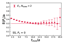
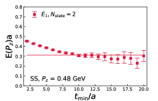
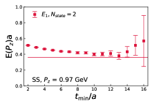
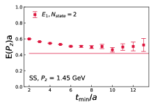
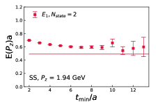
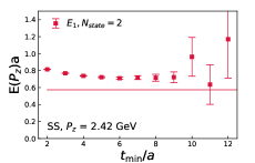
We determined the first excited state energy $E_{1}(\mathbf{P})$ using (1) two-state fits to the SS and SP correlators with fixed value taken from the dispersion relation for $E_{0}$, and (2) by using three-state fits to the SS correlator with fixed $E_{0}$ and imposing a prior on $E_{1}$ with the central value and width of the prior set to the best fit value of $E_{1}$ and its error obtained from the two-state fit to the SP correlator. In Fig. 1, we show the dependence of $E_{1}$ on the fit range $[t_{\rm min},32a]$. Each panel corresponds to the six different momenta $\mathbf{P}=(0,0,P_{z})$, and for each momentum, we have shown the $t_{\rm min}$ dependence of $E_{1}$ from the two-state fit. The best fit values of $E_{1}$ plateau for $t_{s}\geq 10a$. First, we notice that the best fit value of $E_{1}(P_{z}=0)=1.456(92)$ GeV, numerically lies close to the central value of the 1.3 GeV physical mass of the pion radial excitation. This difference of about 200 MeV between the lattice result and physical value for the first excited state is also close to the 150 MeV difference between the mass of pion in our lattice computation and physical pion mass. This observation initially lead us to identify the first excited state on the lattice with the pion radial excitation.

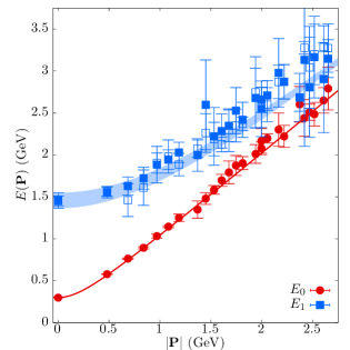
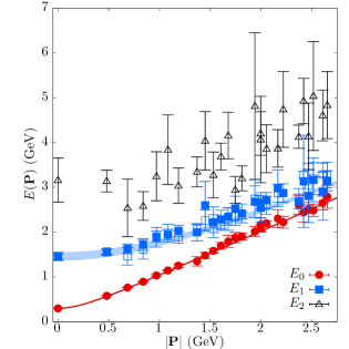
In Fig. 1, we also show the value of $E_{1}(\mathbf{P})$ expected from a single particle dispersion relation with a mass $M_{1}=E_{1}(\mathbf{P}=0)=1.5$ GeV. We find that the best fit values of $E_{1}$ indeed approach the expected continuum values for non-zero momenta. This shows that the first excited state is likely to be a single particle eigenstate, and not a pseudo single particle state that effectively captures a continuum of multiparticle states. In the case of pion, such a possible multiparticle excited state is a three pion state with zero angular momentum and with their total isospin being 1. For our ensemble, we estimate the invariant mass of such a state to be 0.9 GeV, which is much smaller than the first excited state we are finding. One possibility is that the Gaussian source we are using does not have an overlap with the three pion state due to its vastly different delocalized spatial distribution compared to a localized single particle state. To summarize our evidence for observing $\pi(1300)$, we plot the energy-momentum dispersion relation for the ground state and the first excited state in the left panel of Fig. 2. For $E_{1}$, we have shown its estimates from the two-state fits with prior on $E_{0}$, and from three-state fits with prior on $E_{0}$ and $E_{1}$ as described above — these are shown as the blue filled and open squares in the figure, and they can be seen to agree well with each other. We find that both $E_{0}$ and $E_{1}$ agree with their respective single particle dispersion curves. From the three-state fits with priors on $E_{0}$ and $E_{1}$, we were able to estimate the second excited state $E_{2}$, which must capture the tower of excited states above $\pi(1300)$. In the right panel of Fig. 2, we have shown these estimates for $E_{2}$ as the black triangle points, and shown it in comparison to $E_{0}$ and $E_{1}$. We will use results on the spectrum from the three-state fit in the further analysis of three-point functions.

Having demonstrated that the first-excited state observed in our computation is likely to be the first radial excitation of pion, we will henceforth work under the assumption that this is indeed the case, and ask for the properties of this excited state given this justified assumption. In the rest of the paper, we will refer to the first excited state in our lattice computation by $\pi^{\prime}$, rather than calling it as $\pi(1300)$. This is because the mass of the first excitation on our lattice is not 1300 MeV, and for the sake of brevity. We will also simply label the first excited state mass $M_{1}$ as $M_{\pi^{\prime}}$.

III Extraction of excited state bilocal quark bilinear matrix element

Figure 3: The bare matrix element, $h_{11}(z,P_{z})$, for the first excited state of pion is shown using three different types of three-state fits. The panels from left to right correspond to $n_{z}=3,4,5$ momenta respectively. The three types are distinguished by the colored symbols.

In order to determine the required bilocal quark bilinear matrix elements of the boosted $\pi$ and $\pi^{\prime}$, we computed the three-point function

$$C_{\rm 3pt}(z,\tau,t_{s})=\left\langle\pi_{S}(\mathbf{P},t_{s})O(z,\tau)\pi_{S}^{\dagger}(\mathbf{P},0)\right\rangle,$$ (4)

with both the source and sink smeared. The bilocal operator involving quark and antiquark separated spatially by distance $z$ is

$$O(z,\tau) = \sum_{\mathbf{x}}\bigg{[}\overline{u}(x+{\cal L})\gamma_{t}W_{z}(x+{\cal L},x)u(x)$$ (6)

$$\ -\overline{d}(x+{\cal L})\gamma_{t}W_{z}(x+{\cal L},x)d(x)\bigg{]},$$

where $x=(\tau,\mathbf{x})$ with $\tau$ being the time-slice where the operator is inserted, and the quark-antiquark being displaced along the $z$-direction by ${\cal L}=(0,0,0,z)$. The bilocal operator is made gauge-invariant by using a straight Wilson-line $W_{z}$ constructed out of 1-HYP smeared gauge links. Since we are interested only in the parton distribution function in this paper, we used $\mathbf{P}=(0,0,P_{z})$ that is along the direction of Wilson-line for the three-point function computations. We used,

$$P_{z}=\frac{2\pi}{aL}n_{z},$$ (7)

with $n_{z}=0,1,2,3,4,5$. The spectral decomposition of the three-point function

$$C_{\rm 3pt}(t_{s},\tau;z,P_{z})=\sum_{i,j}A_{i}^{*}A_{j}h_{ij}(z,P_{z})e^{-E_{i}(t_{s}-\tau)-E_{j}\tau},$$ (8)

contains information on all the matrix elements between $i$-th and $j$-th states with pion quantum number

$$h_{ij}(z,P_{z})=\langle E_{i},P_{z}|O(z)|E_{j},P_{z}\rangle.$$ (9)

We obtained the values of the amplitudes $|A_{i}|$ and the energies $E_{i}$ from the analyses of $C_{\rm 2pt}$. We fixed them to the central values from the three-state fits. One can extract the matrix elements $h_{ij}$ by fitting the $t_{s}$ and $\tau$ dependence of $C_{\rm 3pt}$ data to the spectral decomposition above, with $h_{ij}$ being the unknown fit parameters. In practice, for the cross-terms such as $A_{0}^{*}A_{1}h_{01}$, we simply treated the real part of such whole factors together as the fit parameters, whereas for the diagonal terms only the magnitudes $|A_{i}|$ enter, and therefore, we were able to resolve the diagonal matrix elements $h_{ii}$ without any phase ambiguity.

We implemented this analysis by first forming the standard ratio

$$R(t_{s},\tau;z,P_{z})\equiv\frac{C_{\rm 3pt}(t_{s},\tau;z,P_{z})}{C_{\rm 2pt}(t_{s};P_{z})},$$ (10)

so that the leading term in this ratio as $t_{s}\to\infty$ is the ground state matrix element $h_{00}$. In Gao et al. (2020), we presented detailed analysis of the ratio $R$ using both the two-state and three-state fits. In that work, we found that a simple two-state fit was enough to obtain $h_{00}$ which was consistent with a more elaborate three-state fit as well as with the summation method. On the one hand, a simple two-state fit is not justified here, as we are interested in the first excited state, and therefore, at least one more state other than the first excited state should be included in the analysis. On the other hand, a full three-state analysis involving 9 independent fit parameters will make the determinations of $h_{11}$ noisy. Therefore, we experimented with variations of the three-state fit by reducing the number of parameters in the fit and by imposing prior on the ground state matrix element $h_{00}$ from the two-state fit. We first performed the full three-state fit with 9 parameters, which we call as the fit of type-1. Then, in a fit of type-2, we imposed a prior on $h_{00}$ keeping all other fit parameters of the full state fit to be free; for the prior and its width we took the value of $h_{00}$ and its statistical error from the two-state analysis of the three-point function. In a fit of type-3, in addition to imposing the prior on $h_{00}$, we also assumed that we can ignore the second-excited state matrix element $h_{22}$, thereby reducing the fit parameters to 8 (or effectively 7, due to the prior). In all the three Ansatze, we kept all the matrix elements which involved the first excited state.

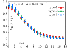
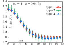
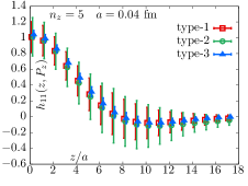
In Fig. 3, we show $\pi^{\prime}$ matrix element, $h_{11}$, as a function of $z$ at the three largest momenta. The different colored symbols are the extrapolations using the above three types of three-state Ansatz. For $n_{z}=3$, the type-1, nine-parameter three-state fit actually performs better than when constraints are imposed. However, this is not true at the higher $n_{z}=4,5$ momenta, which are crucial to ensure that the momenta are larger than the $\pi^{\prime}$ mass. For $n_{z}=3$, the type-2 fit results in noisier estimates of $h_{11}$ compared to type-1, whereas the type-3 fit results are consistent with type-1 results with a slight reduction in errors. Therefore, we find that the type-3 Ansatz leads to a reasonable reduction in the statistical errors with only the assumption that $h_{22}$ matrix element can be ignored. In fact, from the unconstrained type-1 fits, we found that the resulting values for $h_{22}$ were consistent with zero and it was merely making the results noisier. Therefore, the usage of type-3 Ansatz to obtain better estimates of $h_{11}$ seems to be justified. We tried reducing the number of parameters further by ignoring the cross-terms $h_{12}$ and $h_{21}$, but it resulted in unreasonably ultra-precise estimations of $h_{11}$, showing that such constraints rule out most of the parameter space — it would have been a positive outcome if there was a strong theoretical underpinning to ignoring the cross-terms, but in the absence of such a justification, we avoided using such stricter constraints. From the fit results for $n_{z}=5$ shown in the rightmost panel of Fig. 3, the usage of type-3 fit renders $h_{11}$ at this momentum usable. In the analysis of PDF that follows, we will use the values of $h_{11}$ obtained using type-3 Ansatz for the extrapolations, and we will also show results from the type-1 fits to contrast it against.

The bilocal operator $O$ needs to be multiplicatively renormalized Ji et al. (2018); Ishikawa et al. (2017); Green et al. (2018). The details pertaining to renormalization as applied to our computations are described in detail in Izubuchi et al. (2019); Gao et al. (2020). One possibility is to determine the renormalization factors $Z_{\gamma_{t}\gamma_{t}}(z,P^{R})$ in the RI-MOM scheme Stewart and Zhao (2018); Chen et al. (2018); Alexandrou et al. (2011) using off-shell quarks at momentum $P^{R}=(P_{z}^{R},P_{\perp}^{R})$,

$$h^{R}_{\pi^{\prime}\pi^{\prime}}(z,P_{z},P^{R})=\frac{Z_{\gamma_{t}\gamma_{t}}(z,P^{R})h_{11}(z,P_{z})}{Z_{\gamma_{t}\gamma_{t}}(0,P^{R})h_{11}(0,P_{z})},$$ (11)

In addition to the multiplicatively renormalizing the operator, the ratio with the corresponding matrix element at $z=0$, helps reduce lattice corrections and any overall systematical corrections, so that the expectation value of the isospin charge of pion is 1 by construction at all momenta. Another possibility is to form renormalization group invariant ratios Orginos et al. (2017); Izubuchi et al. (2018); Fan et al. (2020); Gao et al. (2020) between the bare matrix elements at two different momenta,

$${\cal M}_{\pi^{\prime}\pi^{\prime}}(z,P_{z},P_{z}^{0})=\left(\frac{h_{11}(z,P_{z})}{h_{11}(z,P_{z}^{0})}\right)\left(\frac{h_{11}(0,P^{0}_{z})}{h_{11}(0,P_{z})}\right).$$ (12)

In the above ratio, the UV divergence of the operator is exactly canceled between the two bare matrix elements. Similar to an improved version of the RI-MOM scheme we defined in Eq. (11), the double ratio at non-zero $z$ and $z=0$ matrix elements in the above equation ensures that the isospin charge is normalized to 1. Since the UV divergence does not depend on the external states, the two matrix elements in the ratio need not be for the same hadron. Therefore, we also construct the following ratio using the ground state pion matrix element as

$${\cal M}_{\pi^{\prime}\pi}(z,P_{z},P_{z}^{0})=\left(\frac{h_{11}(z,P_{z})}{h_{00}(z,P_{z}^{0})}\right)\left(\frac{h_{00}(0,P_{z}^{0})}{h_{11}(0,P_{z})}\right).$$ (13)

For the above ratio, we take our determination of $h_{00}(z,P_{z}^{0})$ from Gao et al. (2020). In the next section, we will discuss the relation of the above matrix elements to the PDF via the one-loop leading-twist perturbative matching.

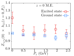
Before performing any double ratio, we can use the $z=0$ renormalized matrix element to perform a simple cross-check. The pion source $\pi(P_{z},t_{s})$ can excite only one unit of the isospin charge, and hence each of the states that occurs in the spectral decomposition of the pion two-point function will carry unit isospin (up to terms due to wrap-around effects, which are negligible for heavy excited states). Therefore, measuring the isospin of our first excited state before imposing any normalization condition serves a cross-check of the excited state extrapolations. In Fig. 4, we show $Z_{\gamma_{t}\gamma_{t}}(z=0,P^{R})h_{11}(z=0,P_{z})$ as a function of $P_{z}$ after renormalization in RI-MOM scheme. It is the isospin charge modulo the quark wavefunction renormalization which is nearly 1 at this lattice spacing Izubuchi et al. (2019). At $P_{z}=0$, our ground-state matrix element determination suffers from 2% lattice periodicity effects Gao et al. (2020), that in turn affects all the fitted parameters in the three-state fit, particularly resulting in a value of $Z_{\gamma_{t}\gamma_{t}}h_{11}$ slightly larger than 1. At all other non-zero $P_{z}$, the extracted isospin of the first excited state is consistent with 1, lending more confidence in the reliability of our extrapolations.

Figure 4: The RI-MOM renormalized local matrix element (mod $Z_{q}\approx 1$) at $z=0$ with $(P^{R}_{z},P^{R}_{\perp})=(1.93,3.34)$ GeV is shown as a function of $P_{z}$ for pion (blue) and $\pi^{\prime}$ (red) as obtained from the three-state type-3 fit. The wrap-around effect present in the three-point function at $P_{z}=0$ is not accounted for in the plot.

IV Comparison of the PDFs of $\pi$ and $\pi^{\prime}$

Figure 5: The excited state matrix elements renormalized in three different schemes (ratios ${\cal M}_{\pi^{\prime}\pi^{\prime}}$, ${\cal M}_{\pi^{\prime}\pi}$ and RI-MOM $h^{R}$ from left to right) are shown as a function of $zP_{z}$. The data points of the same momenta are shown using same colored symbols. The top panels show largest three momenta and the bottom one includes only the largest two. The bands are the fits using the respective leading-twist OPEs to data assuming a two-parameter functional form of the PDF.

We used our estimates of $h_{11}$ from the type-1 and type-3 fits to obtain the PDF of $\pi^{\prime}$. For this, we used the twist-2 OPE expressions Izubuchi et al. (2018) corresponding to the renormalized matrix elements described above. For the RI-MOM matrix element at renormalization scale $P^{R}$, the twist-2 expression is

$$h^{R}_{\pi^{\prime}\pi^{\prime}}(z,P_{z},P^{R})=1+\sum c_{n}^{RI}(\mu,P^{R},z^{2})\langle x^{n}\rangle_{\pi^{\prime}}\frac{(-iP_{z}z)^{n}}{n!},$$ (14)

where the sum above runs over only the even values of $n$ for the valence PDF of the pion and its excitations due to the isospin symmetry. The 1-loop expression for the RI-MOM Wilson coefficients is given in Gao et al. (2020) using results in Constantinou and Panagopoulos (2017); Zhao (2019). The terms $\langle x^{n}\rangle_{\pi^{\prime}}(\mu)=\int_{0}^{1}x^{n}f_{v}(x,\mu)dx$ are the moments  of the valence PDF $f_{v}(x,\mu)$ of the first excited state in the $\overline{\rm MS}$ scheme at factorization scale $\mu$. We will consistently use $\mu=3.2$ GeV for all the determinations in this paper. The twist-2 OPE expression for the ratio scheme Izubuchi et al. (2018) is

$${\cal M}_{\pi^{\prime}\pi^{\prime}}(z,P_{z},P_{z}^{0})=\frac{1+\sum c_{n}(\mu^{2}z^{2})\langle x^{n}\rangle_{\pi^{\prime}}\frac{(-iP_{z}z)^{n}}{n!}}{1+\sum c_{n}(\mu^{2}z^{2})\langle x^{n}\rangle_{\pi^{\prime}}\frac{(-iP^{0}_{z}z)^{n}}{n!}},$$ (15)

using the expressions for the Wilson coefficients $c_{n}$ given in Izubuchi et al. (2018); Radyushkin (2018). Here, we also present results using a variant of the ratio scheme ${\cal M}_{\pi^{\prime}\pi}$ described in the last section, and it has the leading twist expression,

$${\cal M}_{\pi^{\prime}\pi}(z,P_{z},P_{z}^{0})=\frac{1+\sum c_{n}(\mu^{2}z^{2})\langle x^{n}\rangle_{\pi^{\prime}}\frac{(-iP_{z}z)^{n}}{n!}}{1+\sum c_{n}(\mu^{2}z^{2})\langle x^{n}\rangle_{\pi}\frac{(-iP^{0}_{z}z)^{n}}{n!}},$$ (16)

where the moments $\langle x^{n}\rangle_{\pi}$ are those of the ground state pion. We take their values from our analysis of pion on the same ensemble presented in Gao et al. (2020). Since the mass of $\pi^{\prime}$ is about 1.5 GeV, we took care of target mass correction at leading twist by replacing $(P_{z}z)^{n}\to(P_{z}z)^{n}\sum_{k=0}^{n/2}\frac{(n-k)!}{k!(n-2k)!}\left(\frac{M_{\pi^{\prime}}^{2}}{4P_{z}^{2}}\right)^{k}$ in the above expressions Chen et al. (2016b); Radyushkin (2017b). We work under the assumption that any target mass correction that can occur at higher twist are negligible. In order to justify this further, we eventually used only the matrix elements at the two highest momenta corresponding to $P_{z}=1.93$ and 2.42 GeV as we discuss below.

We performed two kinds of analysis. In a model independent analysis, we fitted the renormalized matrix elements spanning a range of $P_{z}>P_{z}^{0}$ and $z\in[z_{\rm min},z_{\rm max}]$ using their respective leading twist expressions above, with the even moments $\langle x^{n}\rangle_{\pi^{\prime}}$ as the independent fit parameters. In the second kind of model dependent analysis, we assumed a two-parameter functional form of valence excited state PDF,

$$f_{v}(x)={\cal N}x^{\alpha}(1-x)^{\beta},$$ (17)

and fitted the resulting moments (which are functions of $\alpha$ and $\beta$) to best describe the $z$ and $zP_{z}$ dependences of the data. This enabled us to reconstruct the $x$-dependent PDF. Since the data for the excited state is noisy, we could not improve the above parametrization by adding additional small-$x$ terms, as we did for the pion in Gao et al. (2020). In the future, one needs to perform a similar analysis with multiple functional forms of the PDF Ansatz to quantify the amount of systematic error.

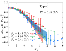
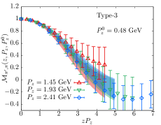
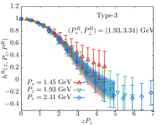
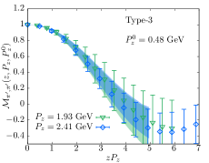
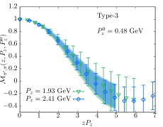
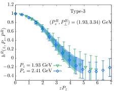
We first describe our reconstruction of the PDF using the two-parameter functional form. In Fig. 5, we put together the renormalized bilocal matrix elements  at different fixed momenta and show them as a function of $zP_{z}$. The left, middle and the right panels are in the two ratio schemes, ${\cal M}_{\pi^{\prime}\pi^{\prime}}$ and ${\cal M}_{\pi^{\prime}\pi}$, and in the RI-MOM scheme with $(P^{R}_{z},P^{R}_{\perp})=(1.93,3.34)$ GeV respectively. We have used the first non-zero momentum, $P_{z}^{0}=0.48$ GeV as the reference momentum to construct the ratios, which is slightly above $\Lambda_{\rm QCD}$ and also contributes minimally to the statistical noise. In the top panels, the data from the three highest momenta are shown, whereas in the bottom panels, only the two highest momenta, $P_{z}=1.93$ and 2.41 GeV, which are larger than the excited state mass of 1.5 GeV are shown. The bands are the expectations based on the best fits using the two-parameter PDF Ansatz; the bands are colored in the same manner as the corresponding data points at different momenta. For the cases shown in the top panel, we performed the fits using all the three momenta shown, and over a range of quark-antiquark separation $z\in[2a,0.6{\ \rm fm}]$. Given the noisy data compared to that of the ground state pion, we could not perform an ideal analysis, where one would want to keep range of $z$ even smaller than what is used here. We skipped $z=a$ to avoid the $(P_{z}a)^{2}$ lattice correction Gao et al. (2020). Overall, the fits can be seen to perform well regardless of the momenta included in the analysis. However, upon a close inspection of the analyses in the top-panel, we find that the evolution of the data with $P_{z}$ at different fixed $zP_{z}$ has opposite trends between the data and the fits; namely, the central values of the data have a decreasing tendency from $P_{z}=1.45$ GeV to 2.41 GeV (albeit well within errors), whereas the fitted bands have the opposite behavior. This indicates the presence of possible higher twist corrections when matrix elements at momentum $P_{z}=1.45$ GeV, which is comparable to the mass of the excited state, is included in the analysis. On the other hand, in the lower-panel, the data at the two highest momenta are compatible with each other and the fitted bands are also seen to be describing the data well. Therefore, to be cautious, we will simply include the data at the two highest momenta in the analysis henceforth.

Figure 6: The valence parton distribution function $f_{v}(x,\mu)$ of $\pi^{\prime}$ at $\mu=3.2$ GeV, as reconstructed from real space matrix elements using fits to simple two-parameter Ansatz $f_{v}(x,\mu)={\cal N}x^{\alpha}(1-x)^{\beta}$. The results for the valence PDF obtained using the bilocal matrix elements in three different renormalization schemes are shown using the different colored bands. The results using type-1 and type-3 matrix elements are shown on the left and right panels respectively. The valence PDF of pion as determined using the same ensemble and analysis methods as used for $\pi^{\prime}$ is shown as the dashed curve for comparison.

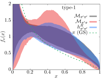
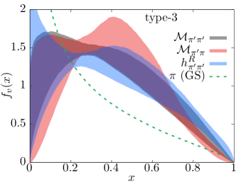
In Fig. 6, we show the $x$-dependent valence PDF of the excited state, $f_{v}(x)$, that is reconstructed based on the two-parameter Ansatz fits in the real-space shown as bands in the bottom panels of Fig. 5. The right panel of Fig. 6 is based on fits to the matrix elements obtained using type-3 extrapolation, whereas the left one is using the type-1 extrapolation. We have compared the PDF determinations as obtained from the fits to the matrix elements in the three different renormalization schemes. For comparison, the central value of the ground state pion PDF from the same ensemble Gao et al. (2020) is shown as the dashed green line. First, the usage of type-1 extrapolated matrix elements results in very noisy PDF that cannot be used to find any hints of structural differences; within the large errors, the excited pion PDF is consistent with the ground state PDF. On the other hand, the usage of type-3 extrapolated matrix element does result in better determined PDFs. Therefore, let us focus on the right panel of Fig. 6. The consistency amongst the estimates from different renormalization schemes, which differ also in their matching formulas, is reassuring. Using ${\cal M}_{\pi^{\prime}\pi^{\prime}}$, we found the PDF is parametrized by $\left\{\alpha,\beta\right\}=\left\{0.4(3),1.1(2)\right\}$. It is very clear that the PDF of the radial excitation is different from the ground state — the excited state PDF is consistently above the pion PDF starting from an intermediate $x\approx 0.3$ to large-$x$. There is a tendency in the excited state PDF to vanish at small-$x$, but it is not conclusive given the errors and also due to possibly large higher-twist effects contaminating the small-$x$ regime. Thus, the overall trend seems to be that the valence PDF of the radial excitation is shifted towards larger-$x$ compared to the ground state valence PDF. This points to smaller momentum fraction being carried by gluons and sea quarks in the radially excited state compared to the pion.

In Fig. 7, we compare the first four valence PDF moments of the radial excitation obtained using the model-dependent and model-independent analyses. The results for $\pi^{\prime}$ from various fitting procedures are shown on the left part of the plot, and the values for the pion, taken from our previous work on the same ensemble Gao et al. (2020), are shown on the right part of the figure. For the model-independent fits, we used the first three even moments $\langle x^{2}\rangle,\langle x^{4}\rangle$ and $\langle x^{6}\rangle$ themselves as the fit parameters. We also imposed the inequality conditions between the valence moments as discussed in Gao et al. (2020). Similar to the PDF Ansatz fits, we present the results of the fits over a $z$-range of $[2a,0.6{\rm fm}]$ in Fig. 7; the model-independent fits to type-1 and type-3 matrix elements are labeled as A and B in Fig. 7. Since we cannot determine the odd moments directly by this model-independent procedure, only the results for $\langle x^{2}\rangle$ and $\langle x^{4}\rangle$ are shown for them. The results for the moments as inferred from the two-parameter fits, using the relation $\langle x^{n}\rangle=\int_{0}^{1}x^{n}f_{v}(x)dx$, are also shown for $\pi^{\prime}$ in Fig. 7; the results from fits to type-1 and type-3 ${\cal M}_{\pi^{\prime}\pi^{\prime}}$ are labeled as C and D, whereas the ones from fits to type-3 ${\cal M}_{\pi^{\prime}\pi}$ matrix element are labeled as E. It is comforting that the PDF Ansatz fits result in values of the even moments that are consistent with those from the model-independent fits. This also gives us the confidence in the indirect determination of the odd moments via this procedure. To justify this indirect method, taking the case of pion where the phenomenological values of the odd moments are known, in Gao et al. (2020), we found that similar analysis via fits to PDF Ansatze resulted in values of the odd moments that agreed reasonably well with the phenomenological values.

Figure 7: The lowest four valence PDF moments of the pion radial excitation $\pi^{\prime}$ is compared with those of the ground state pion $\pi$. For the radial excitation, both the even and odd moments extracted from the two-parameter PDF Ansatz fit are shown along with direct model independent estimates of even moments: (A) model-independent fit to type-1 ${\cal M}_{\pi^{\prime}\pi^{\prime}}$. (B) model-independent fit to type-3 ${\cal M}_{\pi^{\prime}\pi^{\prime}}$. (C) PDF Ansatz fit to type-1 ${\cal M}_{\pi^{\prime}\pi^{\prime}}$. (D) PDF Ansatz fit to type-3 ${\cal M}_{\pi^{\prime}\pi^{\prime}}$. (E) PDF Ansatz fit to type-3 ${\cal M}_{\pi^{\prime}\pi}$. The dashed line connect the central values of $\pi^{\prime}$ moments to that of $\pi$, to aid the eye.

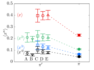
It is at once striking that the moments of $\pi^{\prime}$ are larger than that of the pion, especially in the case of the lowest two-moments $\langle x\rangle$ and $\langle x^{2}\rangle$. Quantitatively, by taking the values of $\left\{\langle x\rangle,\langle x^{2}\rangle\right\}$ from the method “D” in Fig. 7, we see that they are $\left\{0.40(4),0.21(3)\right\}$ for $\pi^{\prime}$, which is to be compared with $\left\{0.2289(96),0.1083(47)\right\}$ for the pion. This is the reason we observed the valence PDF of $\pi^{\prime}$ to be above that of the pion at higher values of $x$. Therefore, at a scale of $3.2$ GeV, only 20% of the $\pi^{\prime}$ momentum fraction comes from gluons and sea quarks, which forms a larger 56% component for the ground state pion. Thus, within the two-parameter PDF Ansatz analysis, it appears that the valence quarks carry almost twice the momentum fraction in the radial excitation of the pion compared to its ground state. This link could simply be a correlation or perhaps be causal, which needs to be investigated using simpler models.

V Conclusions and outlook

In this work, we presented a proof-of-principle computation of the first excited state of the pion determined in a fixed finite volume and at a fixed fine lattice spacing. We argued that the first excited state is most likely to be a single particle state since its energy satisfies a single particle dispersion relation. Also, the mass of the state compares well with the central value of the experimentally observed radial excitation, which is however a resonance in the infinite volume limit. Given the observations, we hypothesized that the first excitation on our lattice is that of the pion radial excitation, $\pi(1300)$. With a reasonable reduction in the number of unknown parameters in the three-state fits to the three-point function involving the bilocal quark bilinear operator, we were able to extract the boosted $\pi(1300)$ matrix elements. We performed a model-independent analysis to obtain the even valence PDF moments, and used model-dependent PDF Ansatz fits to reconstruct the $x$-dependent valence PDF at a scale of $\mu=3.2$ GeV. We found evidences that in indicate that (1) the valence PDF of $\pi(1300)$ consistently lies above that of pion for intermediate and large-$x$ regions, thereby indirectly, implying a reduced role of gluons and sea quarks in the excited state. (2) Quantitatively, the lower moments of $\pi(1300)$ were about twice larger than that of $\pi$.

The present work was meant only as a pilot study towards understanding how the ground and excited states of hadrons differ. Therefore, this study can be made more rigorous in at least three major ways — (1) One could either render the radial excitation to be stable single-particle state by using a larger unphysical pion mass (e.g., Chai et al. (2020)), or one needs to perform a dedicated finite-size scaling study of the excited state PDF in order to make connection with the actual resonance state in the thermodynamic limit. (2) Usage of larger operator basis in two-point functions that will lead to a more sophisticated spectroscopy of pion correlators leading to a more convincing determination of the first excited state as well as its quantum numbers. (3) Incorporating similar techniques for the three-point function for a reliable determination of the excited state matrix element without involving any reduction in number of fit parameters as done here.

As a concluding remark, in the absence of a microscopic theory of the transition from pion to its radial excitation, we propose the following momentum differential as a useful quantity. To motivate the quantity, one can consider a process, such as $\pi^{\prime}\to\pi+({\pi\pi})_{\rm S-wave}$, for a special instance with both $\pi^{\prime}$ and $\pi$ after the transition are at rest in the lab frame, and the difference in their masses carried by other product states. In such an artificially constructed experimental outcome, one could ask how the change, $\Delta P^{+}=(M_{\pi^{\prime}}-M_{\pi})/\sqrt{2}$, compares to the change in the average momentum $\Delta\langle k^{+}\rangle=(M_{\pi^{\prime}}\times 2\langle x\rangle_{\pi^{\prime}}-M_{\pi}\times 2\langle x\rangle_{\pi})/\sqrt{2}$ of the two valence partons in $\pi^{\prime}$ and $\pi$. This motivates the construction of the Lorentz invariant ratio,

$$\zeta=\frac{2M_{\pi^{\prime}}\langle x\rangle_{\pi^{\prime}}-2M_{\pi}\langle x\rangle_{\pi}}{M_{\pi^{\prime}}-M_{\pi}},$$ (18)

as a measure to correlate the structural changes to the differences in the masses. Using $\Delta M=1.2$ GeV, we find that the fraction $\zeta$ ranges from 0.78 to 0.99 given the variations within 1-$\sigma$ errors on the first moments we discussed above. Even if we discount a 2-$\sigma$ variation, the fraction is at least 0.68. Even such a simple-minded modeling of the excitation tells us that the changes to the dynamics of valence parton could play an major role in exciting a pion.

References

- Badier et al. (1983) J. Badier et al. (NA3), Z. Phys. C 18, 281 (1983).
- Betev et al. (1985) B. Betev et al. (NA10), Z. Phys. C 28, 9 (1985).
- Conway et al. (1989) J. Conway et al., Phys. Rev. D 39, 92 (1989).
- Owens (1984) J. Owens, Phys. Rev. D 30, 943 (1984).
- Sutton et al. (1992) P. Sutton, A. D. Martin, R. Roberts, and W. Stirling, Phys. Rev. D 45, 2349 (1992).
- Gluck et al. (1992) M. Gluck, E. Reya, and A. Vogt, Z. Phys. C 53, 651 (1992).
- Gluck et al. (1999) M. Gluck, E. Reya, and I. Schienbein, Eur. Phys. J. C 10, 313 (1999), arXiv:hep-ph/9903288 .
- Wijesooriya et al. (2005) K. Wijesooriya, P. Reimer, and R. Holt, Phys. Rev. C 72, 065203 (2005), arXiv:nucl-ex/0509012 .
- Barry et al. (2018) P. Barry, N. Sato, W. Melnitchouk, and C.-R. Ji, Phys. Rev. Lett. 121, 152001 (2018), arXiv:1804.01965 [hep-ph] .
- Novikov et al. (2020) I. Novikov et al., Phys. Rev. D 102, 014040 (2020), arXiv:2002.02902 [hep-ph] .
- Aicher et al. (2010) M. Aicher, A. Schafer, and W. Vogelsang, Phys. Rev. Lett. 105, 252003 (2010), arXiv:1009.2481 [hep-ph] .
- Nguyen et al. (2011) T. Nguyen, A. Bashir, C. D. Roberts, and P. C. Tandy, Phys. Rev. C 83, 062201 (2011), arXiv:1102.2448 [nucl-th] .
- Chen et al. (2016a) C. Chen, L. Chang, C. D. Roberts, S. Wan, and H.-S. Zong, Phys. Rev. D 93, 074021 (2016a), arXiv:1602.01502 [nucl-th] .
- Cui et al. (2020) Z.-F. Cui, M. Ding, F. Gao, K. Raya, D. Binosi, L. Chang, C. D. Roberts, J. Rodríguez-Quintero, and S. M. Schmidt, Eur. Phys. J. C 80, 1064 (2020).
- Roberts and Schmidt (2020) C. D. Roberts and S. M. Schmidt (2020) arXiv:2006.08782 [hep-ph] .
- de Teramond et al. (2018) G. F. de Teramond, T. Liu, R. S. Sufian, H. G. Dosch, S. J. Brodsky, and A. Deur (HLFHS), Phys. Rev. Lett. 120, 182001 (2018), arXiv:1801.09154 [hep-ph] .
- Ruiz Arriola (2002) E. Ruiz Arriola, Acta Phys. Polon. B 33, 4443 (2002), arXiv:hep-ph/0210007 .
- Broniowski and Ruiz Arriola (2017) W. Broniowski and E. Ruiz Arriola, Phys. Lett. B 773, 385 (2017), arXiv:1707.09588 [hep-ph] .
- Lan et al. (2020) J. Lan, C. Mondal, S. Jia, X. Zhao, and J. P. Vary, Phys. Rev. D 101, 034024 (2020), arXiv:1907.01509 [nucl-th] .
- Bednar et al. (2020) K. D. Bednar, I. C. Cloët, and P. C. Tandy, Phys. Rev. Lett. 124, 042002 (2020), arXiv:1811.12310 [nucl-th] .
- Aguilar et al. (2019) A. C. Aguilar et al., Eur. Phys. J. A 55, 190 (2019), arXiv:1907.08218 [nucl-ex] .
- Adams et al. (2018) B. Adams et al., (2018), arXiv:1808.00848 [hep-ex] .
- Ji (2013) X. Ji, Phys. Rev. Lett. 110, 262002 (2013), arXiv:1305.1539 [hep-ph] .
- Ji (2014) X. Ji, Sci. China Phys. Mech. Astron. 57, 1407 (2014), arXiv:1404.6680 [hep-ph] .
- Radyushkin (2017a) A. Radyushkin, Phys. Rev. D 96, 034025 (2017a), arXiv:1705.01488 [hep-ph] .
- Orginos et al. (2017) K. Orginos, A. Radyushkin, J. Karpie, and S. Zafeiropoulos, Phys. Rev. D 96, 094503 (2017), arXiv:1706.05373 [hep-ph] .
- Braun and Müller (2008) V. Braun and D. Müller, Eur. Phys. J. C 55, 349 (2008), arXiv:0709.1348 [hep-ph] .
- Ma and Qiu (2018a) Y.-Q. Ma and J.-W. Qiu, Phys. Rev. D 98, 074021 (2018a), arXiv:1404.6860 [hep-ph] .
- Ma and Qiu (2018b) Y.-Q. Ma and J.-W. Qiu, Phys. Rev. Lett. 120, 022003 (2018b), arXiv:1709.03018 [hep-ph] .
- Constantinou (2020) M. Constantinou, in 38th International Symposium on Lattice Field Theory (2020) arXiv:2010.02445 [hep-lat] .
- Zhao (2019) Y. Zhao, Int. J. Mod. Phys. A 33, 1830033 (2019), arXiv:1812.07192 [hep-ph] .
- Cichy and Constantinou (2019) K. Cichy and M. Constantinou, Adv. High Energy Phys. 2019, 3036904 (2019), arXiv:1811.07248 [hep-lat] .
- Monahan (2018) C. Monahan, PoS LATTICE2018, 018 (2018), arXiv:1811.00678 [hep-lat] .
- Ji et al. (2020a) X. Ji, Y.-S. Liu, Y. Liu, J.-H. Zhang, and Y. Zhao, (2020a), arXiv:2004.03543 [hep-ph] .
- Gao et al. (2020) X. Gao, L. Jin, C. Kallidonis, N. Karthik, S. Mukherjee, P. Petreczky, C. Shugert, S. Syritsyn, and Y. Zhao, Phys. Rev. D 102, 094513 (2020), arXiv:2007.06590 [hep-lat] .
- Zhang et al. (2019) J.-H. Zhang, J.-W. Chen, L. Jin, H.-W. Lin, A. Schäfer, and Y. Zhao, Phys. Rev. D 100, 034505 (2019), arXiv:1804.01483 [hep-lat] .
- Izubuchi et al. (2019) T. Izubuchi, L. Jin, C. Kallidonis, N. Karthik, S. Mukherjee, P. Petreczky, C. Shugert, and S. Syritsyn, Phys. Rev. D 100, 034516 (2019), arXiv:1905.06349 [hep-lat] .
- Joó et al. (2019) B. Joó, J. Karpie, K. Orginos, A. V. Radyushkin, D. G. Richards, R. S. Sufian, and S. Zafeiropoulos, Phys. Rev. D 100, 114512 (2019), arXiv:1909.08517 [hep-lat] .
- Lin et al. (2020) H.-W. Lin, J.-W. Chen, Z. Fan, J.-H. Zhang, and R. Zhang, (2020), arXiv:2003.14128 [hep-lat] .
- Sufian et al. (2019) R. S. Sufian, J. Karpie, C. Egerer, K. Orginos, J.-W. Qiu, and D. G. Richards, Phys. Rev. D 99, 074507 (2019), arXiv:1901.03921 [hep-lat] .
- Sufian et al. (2020) R. S. Sufian, C. Egerer, J. Karpie, R. G. Edwards, B. Joó, Y.-Q. Ma, K. Orginos, J.-W. Qiu, and D. G. Richards, Phys. Rev. D 102, 054508 (2020), arXiv:2001.04960 [hep-lat] .
- Karthik (2021) N. Karthik, (2021), arXiv:2101.02224 [hep-lat] .
- Braun et al. (2019) V. M. Braun, A. Vladimirov, and J.-H. Zhang, Phys. Rev. D 99, 014013 (2019), arXiv:1810.00048 [hep-ph] .
- Liu and Chen (2020) W.-Y. Liu and J.-W. Chen, (2020), arXiv:2010.06623 [hep-ph] .
- Ji et al. (2020b) X. Ji, Y. Liu, A. Schäfer, W. Wang, Y.-B. Yang, J.-H. Zhang, and Y. Zhao, (2020b), arXiv:2008.03886 [hep-ph] .
- Roberts (2020) C. D. Roberts, Symmetry 12, 1468 (2020), arXiv:2009.04011 [hep-ph] .
- McNeile and Michael (2006) C. McNeile and C. Michael (UKQCD), Phys. Lett. B 642, 244 (2006), arXiv:hep-lat/0607032 .
- Mastropas and Richards (2014) E. V. Mastropas and D. G. Richards (Hadron Spectrum), Phys. Rev. D 90, 014511 (2014), arXiv:1403.5575 [hep-lat] .
- Holl et al. (2004) A. Holl, A. Krassnigg, and C. D. Roberts, Phys. Rev. C 70, 042203 (2004), arXiv:nucl-th/0406030 .
- Li et al. (2016) B. L. Li, L. Chang, F. Gao, C. D. Roberts, S. M. Schmidt, and H. S. Zong, Phys. Rev. D 93, 114033 (2016), arXiv:1604.07415 [nucl-th] .
- Chai et al. (2020) Y. Chai et al., Phys. Rev. D 102, 014508 (2020), arXiv:2002.12044 [hep-lat] .
- Dudek et al. (2012) J. Dudek et al., Eur. Phys. J. A 48, 187 (2012), arXiv:1208.1244 [hep-ex] .
- Tanabashi et al. (2018) M. Tanabashi et al. (Particle Data Group), Phys. Rev. D 98, 030001 (2018).
- Bali et al. (2016) G. S. Bali, B. Lang, B. U. Musch, and A. Schäfer, Phys. Rev. D 93, 094515 (2016), arXiv:1602.05525 [hep-lat] .
- Ji et al. (2018) X. Ji, J.-H. Zhang, and Y. Zhao, Phys. Rev. Lett. 120, 112001 (2018), arXiv:1706.08962 [hep-ph] .
- Ishikawa et al. (2017) T. Ishikawa, Y.-Q. Ma, J.-W. Qiu, and S. Yoshida, Phys. Rev. D 96, 094019 (2017), arXiv:1707.03107 [hep-ph] .
- Green et al. (2018) J. Green, K. Jansen, and F. Steffens, Phys. Rev. Lett. 121, 022004 (2018), arXiv:1707.07152 [hep-lat] .
- Stewart and Zhao (2018) I. W. Stewart and Y. Zhao, Phys. Rev. D 97, 054512 (2018), arXiv:1709.04933 [hep-ph] .
- Chen et al. (2018) J.-W. Chen, T. Ishikawa, L. Jin, H.-W. Lin, Y.-B. Yang, J.-H. Zhang, and Y. Zhao, Phys. Rev. D 97, 014505 (2018), arXiv:1706.01295 [hep-lat] .
- Alexandrou et al. (2011) C. Alexandrou, M. Constantinou, T. Korzec, H. Panagopoulos, and F. Stylianou, Phys. Rev. D 83, 014503 (2011), arXiv:1006.1920 [hep-lat] .
- Izubuchi et al. (2018) T. Izubuchi, X. Ji, L. Jin, I. W. Stewart, and Y. Zhao, Phys. Rev. D 98, 056004 (2018), arXiv:1801.03917 [hep-ph] .
- Fan et al. (2020) Z. Fan, X. Gao, R. Li, H.-W. Lin, N. Karthik, S. Mukherjee, P. Petreczky, S. Syritsyn, Y.-B. Yang, and R. Zhang, Phys. Rev. D 102, 074504 (2020), arXiv:2005.12015 [hep-lat] .
- Constantinou and Panagopoulos (2017) M. Constantinou and H. Panagopoulos, Phys. Rev. D 96, 054506 (2017), arXiv:1705.11193 [hep-lat] .
- Radyushkin (2018) A. Radyushkin, Phys. Lett. B 781, 433 (2018), arXiv:1710.08813 [hep-ph] .
- Chen et al. (2016b) J.-W. Chen, S. D. Cohen, X. Ji, H.-W. Lin, and J.-H. Zhang, Nucl. Phys. B 911, 246 (2016b), arXiv:1603.06664 [hep-ph] .
- Radyushkin (2017b) A. Radyushkin, Phys. Lett. B 770, 514 (2017b), arXiv:1702.01726 [hep-ph] .
- Braun et al. (1995) V. Braun, P. Gornicki, and L. Mankiewicz, Phys. Rev. D 51, 6036 (1995), arXiv:hep-ph/9410318 .