Simulation of first-passage times
for alternating Brownian motions

Abstract

The first-passage-time problem for a Brownian motion with alternating infinitesimal moments through a constant boundary is considered under the assumption that the time intervals between consecutive changes of these moments are described by an alternating renewal process. Bounds to the first-passage-time density and distribution function are obtained, and a simulation procedure to estimate first-passage-time densities is constructed. Examples of applications to problems in environmental sciences and mathematical finance are also provided.

Keywords: Brownian motion; alternating infinitesimal moments; renewal process; first-passage time; simulation.

AMS 2000 Subject Classification: 60J65, 60G40, 93E30.

1 Introduction

Stochastic processes and related first-passage-time (FPT) problems have received increasing attention in the literature within the context of model building in biology (see, for instance, Ricciardi et al., 1999, and references therein). Consequently, efforts have also been directed towards the design of computational methods suitable to estimate FPT densities, in particular for general Gaussian processes (see Di Nardo et al., 2001) and for diffusion processes (see references in Ricciardi et al., 1999; in particular, Buonocore et al., 1987, and Giorno et al., 1989).

Here we address the FPT problem through a constant boundary for a model of random motion on the real line consisting of a Brownian process whose infinitesimal moments alternate between fixed values at the occurrence times of an alternating renewal process. Our approach has a twofold aim: (i) to obtain bounds to the FPT density and distribution function conditional on the initial infinitesimal moments and initial state, and (ii) to set up a simulation procedure for the estimation of FPT densities.

A mathematical specification of the random motion will be given in Section 2, where the key definitions related to the FPT problem through a constant boundary will also be recalled. In Section 3, bounds to the FPT density and distribution function will be obtained, and an example of bimodal FPT pdf will be provided. In Section 4 a procedure to generate FPTs will be constructed by simulating sample paths of the Brownian motion at the random times when the infinitesimal moments alternate. Our simulation procedure is specifically based on the independent increments property of the Brownian motion and on the available closed form expression of its FPT density through a constant boundary. In Section 5 two applications to environmental sciences and to mathematical finance, respectively, will be provided. In the Appendix, the involved probabilistic justification of some crucial steps of the simulation algorithm will be presented.

We wish to mention that Brownian motion with alternating infinitesimal moments might provide a fundamental ingredient for the construction of a viable model of a phenomenon of great biological relevance: the dynamics of the motion of myosin heads along actin filaments, that is responsible for the force generation underlying muscle contraction. Highly innovative and accurate measurements have indeed proved that such motion consists of small steps randomly alternating in direction (see Cyranoski, 2000).

2 Brownian motion with alternating behaviors

We consider a Brownian motion on the real line characterized by alternating behaviors, in the sense that its infinitesimal moments switch between fixed values at certain random times. More precisely, starting from state $x_{0}$ at time $0$, the motion undergoes two alternating regimes during random periods governed by an alternating renewal process $\{\delta(t),t\geq 0\}$, defined on states $1$ and $2$. Here, we assume that $\delta(t)$ is governed by two independent sequences of non-negative iid random variables $\{U_{1},U_{2},\ldots\}$ and $\{D_{1},D_{2},\ldots\}$. We assume that during the periods of random lengths $U_{i}$, $i=1,2,\ldots$, one has $\delta(t)=1$ while the Brownian motion has drift $\mu_{1}\geq 0$ and infinitesimal variance $\sigma_{1}^{2}>0$; instead, during the periods of random lengths $D_{i}$, $i=1,2,\ldots$, it is $\delta(t)=2$, and the infinitesimal moments take values $\mu_{2}\leq 0$ and $\sigma_{2}^{2}>0$. We assume that at time $0$ the initial regime can be arbitrarily specified as $\delta(0)=1$ or $\delta(0)=2$. Therefore, the periods of random lengths characterizing the alternating motion are $U_{1},D_{1},U_{2},D_{2},\ldots$ if $\delta(0)=1$, and $D_{1},U_{1},D_{2},U_{2},\ldots$ if $\delta(0)=2$. Consequently, for all $t>0$ we have:

$$\delta(t)=\left\{\begin{array}[]{ll}\displaystyle\sum_{n=1}^{+\infty}\hbox{\bf 1}_{\{T_{2n-2}\leq t<T_{2n-1}\}}+2\displaystyle\sum_{n=1}^{+\infty}\hbox{\bf 1}_{\{T_{2n-1}\leq t<T_{2n}\}}&{\rm if}\;\delta(0)=1,\\ \hfill&\hfill\\ 2\displaystyle\sum_{n=1}^{+\infty}\hbox{\bf 1}_{\{T_{2n-2}\leq t<T_{2n-1}\}}+\displaystyle\sum_{n=1}^{+\infty}\hbox{\bf 1}_{\{T_{2n-1}\leq t<T_{2n}\}}&{\rm if}\;\delta(0)=2,\end{array}\right.$$

where $T_{0}=0$ and $T_{n}$, $n=1,2,\ldots$, denotes the $n$-th random instants in which the infinitesimal moments change values, with

$$T_{2n-1}=T_{2n-2}+\left\{\begin{array}[]{ll}U_{n}&{\rm if}\;\delta(0)=1,\\ \hfill&\hfill\\ D_{n}&{\rm if}\;\delta(0)=2,\end{array}\right.\qquad T_{2n}=T_{2n-1}+\left\{\begin{array}[]{ll}D_{n}&{\rm if}\;\delta(0)=1,\\ \hfill&\hfill\\ U_{n}&{\rm if}\;\delta(0)=2.\end{array}\right.$$ (1)

Denoting by $\{X(t),t\geq 0\}$ the stochastic process that describes the motion, we thus have:

$$X(t)=x_{0}+\int_{0}^{t}\mu(\tau)\,{\rm d}\tau+\sigma(t)\,B(t),\qquad t>0.$$ (2)

with $X(0)=x_{0}\in\vbox{\hbox to8.9pt{I\hskip-2.1ptR\hfil}}$,

$$\mu(t)=\left\{\begin{array}[]{ll}\mu_{1},&\hbox{if }\delta(t)=1\\ \mu_{2},&\hbox{if }\delta(t)=2,\end{array}\right.\qquad\sigma(t)=\left\{\begin{array}[]{ll}\sigma_{1},&\hbox{if }\delta(t)=1\\ \sigma_{2},&\hbox{if }\delta(t)=2,\end{array}\right.$$ (3)

and where $\{B(t),t\geq 0\}$ is a standard Brownian motion that is assumed to be independent of $\{\delta(t)\}$.

For all $x\in\vbox{\hbox to8.9pt{I\hskip-2.1ptR\hfil}}$, $t\geq 0$, $x_{0}\in\vbox{\hbox to8.9pt{I\hskip-2.1ptR\hfil}}$ and $k=1,2$ let us set

$$\begin{array}[]{l}f_{k}(x,t\,|\,x_{0}):=\displaystyle{\partial\over\partial x}\mathop{\rm P}\{X(t)\leq x,\delta(t)=1\,|\,X(0)=x_{0},\delta(0)=k\},\vspace{0.1cm}\\ b_{k}(x,t\,|\,x_{0}):=\displaystyle{\partial\over\partial x}\mathop{\rm P}\{X(t)\leq x,\delta(t)=2\,|\,X(0)=x_{0},\delta(0)=k\}.\end{array}$$

Thus, $f_{k}$ is the pdf of $X(t)$ when the drift is positive, while $b_{k}$ relates to negative drift, both conditional on initial state $x_{0}$ and on initial regime $k$. Hence, for all $x\in\vbox{\hbox to8.9pt{I\hskip-2.1ptR\hfil}}$ and $t\geq 0$

$$p_{k}(x,t\,|\,x_{0}):=f_{k}(x,t\,|\,x_{0})+b_{k}(x,t\,|\,x_{0})$$

is the pdf of $X(t)$ conditional on $X(0)=x_{0}\in\vbox{\hbox to8.9pt{I\hskip-2.1ptR\hfil}}$ and on $\delta(0)=k\in\{1,2\}$.

Let us now address the FPT problem through a boundary $\beta$ for $X(t)$ starting from $x_{0}\in\vbox{\hbox to8.9pt{I\hskip-2.1ptR\hfil}}$ at time $0$. We assume $\beta>x_{0}$. (Case $\beta<x_{0}$ can be consequently analyzed by resorting to symmetry considerations). Let

$$T_{k}^{X}=\inf\{t>0:X(t)>\beta\},\qquad X(0)=x_{0},\;\delta(0)=k\in\{1,2\}$$ (4)

be the FPT of $\{X(t)\}$ through $\beta$ from below. We denote by

$$H_{k}(\beta,t\,|\,x_{0}):=\mathop{\rm P}\left\{T_{k}^{X}\leq t\,\Big{|}\,X(0)=x_{0},\delta(0)=k\right\}$$ (5)

its cumulative distribution function (cdf) and by

$$h_{k}(\beta,t\,|\,x_{0}):=\displaystyle{\partial\over\partial t}H_{k}(\beta,t\,|\,x_{0})$$ (6)

the corresponding pdf. For $k=1,2$ let now

$$W_{k}(t):=x_{0}+\mu_{k}\,t+\sigma_{k}\,B(t),\qquad t\geq 0,$$ (7)

be the Wiener process characterized by drift $\mu_{k}\in\vbox{\hbox to8.9pt{I\hskip-2.1ptR\hfil}}$ and infinitesimal variance $\sigma^{2}_{k}>0$, with initial state $W_{k}(0)=x_{0}\in\vbox{\hbox to8.9pt{I\hskip-2.1ptR\hfil}}\,$, and

$$T_{k}^{W}=\inf\{t>0:W_{k}(t)>\beta\},\qquad W_{k}(0)=x_{0}$$ (8)

be the upward FPT of $W_{k}(t)$ from $x_{0}$ through the boundary $\beta$, with $\beta>x_{0}$.

In the foregoing, use of the following formulas will be made:

(i)  FPT cdf of $W_{k}(t)$ through $\beta$:

$$G_{k}(\beta,t\,|\,x_{0})\!\!\!\! = \!\!\!\!\mathop{\rm P}\left\{T_{k}^{W}\leq t\,\Big{|}\,W(0)=x_{0}\right\}$$ (9)

$$= \!\!\!\!\Phi\left(-\displaystyle{\beta-x_{0}-\mu_{k}t\over\sigma_{k}\sqrt{t}}\right)+e^{2\mu_{k}(\beta-x_{0})/\sigma_{k}^{2}}\,\Phi\left(-\displaystyle{\beta-x_{0}+\mu_{k}t\over\sigma_{k}\sqrt{t}}\right),$$

where $\Phi(x)=(2\pi)^{-1/2}\int_{-\infty}^{x}e^{-y^{2}/2}\,dy$; note that $\displaystyle\lim_{t\to+\infty}G_{k}(\beta,t\,|\,x_{0})=1$ for $\mu_{k}\geq 0$ and        $\displaystyle\lim_{t\to+\infty}G_{k}(\beta,t\,|\,x_{0})=\exp\{2\mu_{k}(\beta-x_{0})/\sigma^{2}_{k}\}$ for $\mu_{k}\leq 0$;

(ii)   FPT pdf of $W_{k}(t)$ through $\beta$:

$$g_{k}(\beta,t\,|\,x_{0})={d\over dt}\mathop{\rm P}\left\{T_{k}^{W}\leq t\,\Big{|}\,W(0)=x_{0}\right\}={\beta-x_{0}\over\sqrt{2\pi\sigma^{2}_{k}t^{3}}}\,\exp\left\{-{(\beta-x_{0}-\mu_{k}t)^{2}\over 2\sigma^{2}_{k}t}\right\};$$ (10)

(iii)  the $\beta$-avoiding pdf of $W_{k}(t)$:

$$\alpha_{k}(x,t\,|\,x_{0})={\partial\over\partial x}\mathop{\rm P}\left\{W(t)\leq x,T_{k}^{W}>t\,\Big{|}\,W(0)=x_{0}\right\}$$

$$\hskip 14.22636pt={1\over\sqrt{2\pi\sigma_{k}^{2}t}}\,\exp\left\{-{(x-x_{0}-{\mu_{k}}t)^{2}\over 2\sigma^{2}_{k}t}\right\}\left[1-\exp\left\{-{2\over\sigma^{2}_{k}t}\,(\beta-x)\,(\beta-x_{0})\right\}\right].$$ (11)

3 Bounds to FPT pdf and cdf

In this section we obtain bounds to the FPT pdf (6) and cdf (5). Hereafter we shall denote by $F_{U}(t)=\mathop{\rm P}(U_{n}\leq t)$ and $F_{D}(t)=\mathop{\rm P}(D_{n}\leq t)$ the cdf’s of random times $U_{n}$ and $D_{n}$, $n=1,2,\ldots$, respectively, and by $\overline{F}_{U}(t)=1-F_{U}(t)$ and $\overline{F}_{D}(t)=1-F_{D}(t)$ the corresponding survival functions.

3.1 Lower bounds to FPT densities

First of all we point out the existence of some renewal-type equations involving the FPT pdf’s $h_{k}$ defined in (6).

Lemma 3.1

For all $t>0$ and $\beta>x_{0}$ the following equations hold:

$$h_{1}(\beta,t\,|\,x_{0})=\overline{F}_{U}(t)\,g_{1}(\beta,t\,|\,x_{0})+\displaystyle\int_{0}^{t}\int_{-\infty}^{\beta}h_{2}(\beta,t-u\,|\,x)\,\alpha_{1}(x,u\,|\,x_{0})\,{\rm d}x\,{\rm d}F_{U}(u),$$ (12)

$$h_{2}(\beta,t\,|\,x_{0})=\overline{F}_{D}(t)\,g_{2}(\beta,t\,|\,x_{0})+\displaystyle\int_{0}^{t}\int_{-\infty}^{\beta}h_{1}(\beta,t-u\,|\,x)\,\alpha_{2}(x,u\,|\,x_{0})\,{\rm d}x\,{\rm d}F_{D}(u).$$ (13)

• Conditioning on $U_{1}$, from (6) we have:

  $$h_{1}(\beta,t\,|\,x_{0})\,{\rm d}t=\int_{0}^{t}\mathop{\rm P}\left\{T_{1}^{X}\in{\rm d}t\,\Big{|}\,U_{1}=u,X(0)=x_{0},\delta(0)=1\right\}{\rm d}F_{U}(u)+\overline{F}_{U}(t)\,g_{1}(\beta,t\,|\,x_{0})\,{\rm d}t.$$

  Eq. (12) then follows noting that, for $0<u<t$, there results:

  $$\mathop{\rm P}\left\{T_{1}^{X}\in{\rm d}t\,\Big{|}\,U_{1}=u,X(0)=x_{0},\delta(0)=1\right\}=\int_{-\infty}^{\beta}h_{2}(\beta,t-u\,|\,x)\,\alpha_{1}(x,u\,|\,x_{0})\,{\rm d}x.$$

  The proof of (13) can be similarly obtained.  

Lower bounds to FPT densities $h_{k}$ will now be obtained.

Theorem 3.1

For all $t>0$ and $\beta>x_{0}$ we have:

$$\begin{array}[]{l}h_{1}(\beta,t\,|\,x_{0})\geq\overline{F}_{U}(t)\,g_{1}(\beta,t\,|\,x_{0})+\displaystyle\int_{0}^{t}\overline{F}_{D}(t-u)\,I_{1}(u,t\,|\,x_{0})\,{\rm d}F_{U}(u),\vspace{0.1cm}\\ h_{2}(\beta,t\,|\,x_{0})\geq\overline{F}_{D}(t)\,g_{2}(\beta,t\,|\,x_{0})+\displaystyle\int_{0}^{t}\overline{F}_{U}(t-u)\,I_{2}(u,t\,|\,x_{0})\,{\rm d}F_{D}(u).\end{array}$$ (14)

where, for $0<u<t$,

$$\begin{array}[]{l}I_{1}(u,t\,|\,x_{0}):=\displaystyle\int_{-\infty}^{\beta}g_{2}(\beta,t-u\,|\,x)\,\alpha_{1}(x,u\,|\,x_{0})\,{\rm d}x\,,\vspace{0.1cm}\\ \hskip 59.75095pt=\displaystyle\frac{1}{\sqrt{2\pi[u\sigma_{1}^{2}+(t-u)\sigma_{2}^{2}]^{3}}}\left[A_{-}(t,u)+A_{+}(t,u)\right]\,,\vspace{0.1cm}\\ I_{2}(u,t\,|\,x_{0}):=\displaystyle\int_{-\infty}^{\beta}g_{1}(\beta,t-u\,|\,x)\,\alpha_{2}(x,u\,|\,x_{0})\,{\rm d}x\,,\vspace{0.1cm}\\ \hskip 65.44142pt=\displaystyle\frac{1}{\sqrt{2\pi[u\sigma_{2}^{2}+(t-u)\sigma_{1}^{2}]^{3}}}\left[B_{-}(t,u)+B_{+}(t,u)\right]\,,\end{array}$$ (15)

with

$$A_{\pm}(t,u)=[(\beta-x_{0})\sigma_{2}^{2}\pm u(\mu_{1}\sigma_{2}^{2}-\mu_{2}\sigma_{1}^{2})]$$

$$\hskip 45.52458pt\times\exp\left\{{-\frac{[-\mu_{1}u-\mu_{2}(t-u)\mp(\beta-x_{0})]^{2}}{2[u\sigma_{1}^{2}+(t-u)\sigma_{2}^{2}]}}\right\}\exp\left\{-\frac{(\mu_{1}\pm\mu_{1})(\beta-x_{0})}{\sigma_{1}^{2}}\right\}$$

$$\hskip 45.52458pt\times\Phi\left(-[u(\mu_{1}\sigma_{2}^{2}-\mu_{2}\sigma_{1}^{2})\pm(\beta-x_{0})\sigma_{2}^{2}]\sqrt{\frac{t-u}{\sigma_{1}^{2}\sigma_{2}^{2}u[u\sigma_{1}^{2}+(t-u)\sigma_{2}^{2}]}}\right)$$

and

$$B_{\pm}(t,u)=[(\beta-x_{0})\sigma_{1}^{2}\pm u(\mu_{1}\sigma_{2}^{2}-\mu_{2}\sigma_{1}^{2})]$$

$$\hskip 45.52458pt\times\exp\left\{{-\frac{[-\mu_{1}(t-u)-\mu_{2}u\pm(\beta-x_{0})]^{2}}{2[u\sigma_{2}^{2}+(t-u)\sigma_{1}^{2}]}}\right\}\exp\left\{\frac{(\mu_{2}\mp\mu_{2})(\beta-x_{0})}{\sigma_{2}^{2}}\right\}$$

$$\hskip 45.52458pt\times\Phi\left([u(\mu_{1}\sigma_{1}^{2}-\mu_{2}\sigma_{2}^{2})\pm(\beta-x_{0})\sigma_{1}^{2}]\sqrt{\frac{t-u}{\sigma_{1}^{2}\sigma_{2}^{2}u[u\sigma_{2}^{2}+(t-u)\sigma_{1}^{2}]}}\right).$$

• Substituting (13) in (12), for all $t>0$ and $\beta>x_{0}$ we have

  $$\begin{array}[]{l}h_{1}(\beta,t\,|\,x_{0})=\overline{F}_{U}(t)\,g_{1}(\beta,t\,|\,x_{0})+\displaystyle\int_{0}^{t}\int_{-\infty}^{\beta}\overline{F}_{D}(t-u)\,g_{2}(\beta,t-u\,|\,x)\,\alpha_{1}(x,u\,|\,x_{0})\,{\rm d}x\,{\rm d}F_{U}(u)\\ +\displaystyle\int_{0}^{t}\int_{-\infty}^{\beta}\left[\int_{0}^{t-u}\int_{-\infty}^{\beta}h_{1}(\beta,t-u-v\,|\,y)\,\alpha_{2}(y,v\,|\,x)\,{\rm d}y\,{\rm d}F_{D}(v)\right]\alpha_{1}(x,u\,|\,x_{0})\,{\rm d}x\,{\rm d}F_{U}(u).\end{array}$$ (16)

  Similarly, substitution of (12) in (13) yields:

  $$\begin{array}[]{l}h_{2}(\beta,t\,|\,x_{0})=\overline{F}_{D}(t)\,g_{2}(\beta,t\,|\,x_{0})+\displaystyle\int_{0}^{t}\int_{-\infty}^{\beta}\overline{F}_{U}(t-u)\,g_{1}(\beta,t-u\,|\,x)\,\alpha_{2}(x,u\,|\,x_{0})\,{\rm d}x\,{\rm d}F_{D}(u)\\ +\displaystyle\int_{0}^{t}\int_{-\infty}^{\beta}\left[\int_{0}^{t-u}\int_{-\infty}^{\beta}h_{2}(\beta,t-u-v\,|\,y)\,\alpha_{1}(y,v\,|\,x)\,{\rm d}y\,{\rm d}F_{U}(v)\right]\alpha_{2}(x,u\,|\,x_{0})\,{\rm d}x\,{\rm d}F_{D}(u).\end{array}$$ (17)

  Hence, from Eqs. (16) and (17) we obtain

  $$h_{1}(\beta,t\,|\,x_{0})\geq\overline{F}_{U}(t)\,g_{1}(\beta,t\,|\,x_{0})+\int_{0}^{t}\int_{-\infty}^{\beta}\overline{F}_{D}(t-u)\,g_{2}(\beta,t-u\,|\,x)\,\alpha_{1}(x,u\,|\,x_{0})\,{\rm d}x\,{\rm d}F_{U}(u),$$

  $$h_{2}(\beta,t\,|\,x_{0})\geq\overline{F}_{D}(t)\,g_{2}(\beta,t\,|\,x_{0})+\int_{0}^{t}\int_{-\infty}^{\beta}\overline{F}_{U}(t-u)\,g_{1}(\beta,t-u\,|\,x)\,\alpha_{2}(x,u\,|\,x_{0})\,{\rm d}x\,{\rm d}F_{D}(u).$$

  Recalling (10) and (11), after some calculations Eqs. (14) follow.  

We point out the following probabilistic interpretation of the functions defined in (15): for $k=1,2$, $I_{k}(u,t\,|\,x_{0})$ identifies with the FPT density through $\beta$, when the initial infinitesimal moments are $\mu_{k}$ and $\sigma^{2}_{k}$, with initial state $x_{0}$, jointly with the condition that up to time $t$ only one inversion of infinitesimal moments has occurred, such an inversion having occurred at time $u$.

3.2 Bounds to FPT distribution functions

We shall now obtain upper and lower bounds to the FPT cdf defined in (5). To this purpose we prove that two integral equations for $H_{1}$ and $H_{2}$ hold.

Theorem 3.2

For all $t>0$ and $\beta>x_{0}$ the following equalities hold:

$$H_{1}(\beta,t\,|\,x_{0})=\overline{F}_{U}(t)\,G_{1}(\beta,t\,|\,x_{0})+\int_{0}^{t}G_{1}(\beta,u\,|\,x_{0})\,{\rm d}F_{U}(u)$$

$$\;+\int_{0}^{t}{\rm d}F_{U}(u)\int_{-\infty}^{\beta}\Bigg{\{}\overline{F}_{D}(t-u)\,G_{2}(\beta,t-u\,|\,x)+\int_{0}^{t-u}G_{2}(\beta,v\,|\,x)\,{\rm d}F_{D}(v)$$

$$\;+\int_{0}^{t-u}{\rm d}F_{D}(v)\int_{-\infty}^{\beta}\alpha_{2}(y,v\,|\,x)\,H_{1}(\beta,t-u-v\,|\,y)\,{\rm d}y\Bigg{\}}\alpha_{1}(x,u\,|\,x_{0})\,{\rm d}x,$$ (18)

$$H_{2}(\beta,t\,|\,x_{0})=\overline{F}_{D}(t)\,G_{2}(\beta,t\,|\,x_{0})+\int_{0}^{t}G_{2}(\beta,u\,|\,x_{0})\,{\rm d}F_{D}(u)$$

$$\;+\int_{0}^{t}{\rm d}F_{D}(u)\int_{-\infty}^{\beta}\Bigg{\{}\overline{F}_{U}(t-u)\,G_{1}(\beta,t-u\,|\,x)+\int_{0}^{t-u}G_{1}(\beta,v\,|\,x)\,{\rm d}F_{U}(v)$$

$$\;+\int_{0}^{t-u}{\rm d}F_{U}(v)\int_{-\infty}^{\beta}\alpha_{1}(y,v\,|\,x)\,H_{2}(\beta,t-u-v\,|\,y)\,{\rm d}y\Bigg{\}}\alpha_{2}(x,u\,|\,x_{0})\,{\rm d}x.$$ (19)

• Conditioning on $U_{1}$, from Eq. (5) we have:

  $$H_{1}(\beta,t\,|\,x_{0})=\int_{0}^{t}\mathop{\rm P}\left(T_{1}^{X}\leq t\,\Big{|}\,U_{1}=u,X(0)=x_{0},\delta(0)=1\right)\,{\rm d}F_{U}(u)+\overline{F}_{U}(t)\,G_{1}(\beta,t\,|\,x_{0}).$$ (20)

  Hence, by noting that for $0<u<t$ there holds

  $$\mathop{\rm P}\left(T_{1}^{X}\leq t\,|\,U_{1}=u\right)\!\!\!\! = \!\!\!\!\mathop{\rm P}\left(T_{1}^{X}\leq u\,|\,U_{1}=u\right)+\mathop{\rm P}\left(u<T_{1}^{X}\leq t\,|\,U_{1}=u\right)$$ (21)

  $$= \!\!\!\!G_{1}(\beta,u\,|\,x_{0})+\int_{-\infty}^{\beta}\alpha_{1}(x,u\,|\,x_{0})\,H_{2}(\beta,t-u\,|\,x)\,{\rm d}x$$

  one obtains:

  $$H_{1}(\beta,t\,|\,x_{0})\!\!\!\! = \!\!\!\!\overline{F}_{U}(t)\,G_{1}(\beta,t\,|\,x_{0})+\int_{0}^{t}G_{1}(\beta,u\,|\,x_{0})\,{\rm d}F_{U}(u)$$ (22)

  $$+ \!\!\!\!\int_{0}^{t}\int_{-\infty}^{\beta}\alpha_{1}(x,u\,|\,x_{0})\,H_{2}(\beta,t-u\,|\,x)\,{\rm d}x\,{\rm d}F_{U}(u).$$

  By a similar argument, one is led to the following equation:

  $$H_{2}(\beta,t\,|\,x_{0})\!\!\!\! = \!\!\!\!\overline{F}_{D}(t)\,G_{2}(\beta,t\,|\,x_{0})+\int_{0}^{t}G_{2}(\beta,u\,|\,x_{0})\,{\rm d}F_{D}(u)$$ (23)

  $$+ \!\!\!\!\int_{0}^{t}\int_{-\infty}^{\beta}\alpha_{2}(x,u\,|\,x_{0})\,H_{1}(\beta,t-u\,|\,x)\,{\rm d}x\,{\rm d}F_{D}(u).$$

  Substitution of the right-hand-side of (23) into (22), and viceversa, finally yields Eqs. (18) and (19).  

The following theorem provides upper and lower bounds to the FPT cdf’s $H_{1}$ and $H_{2}$.

Theorem 3.3

For all $t>0$ and $\beta>x_{0}$ there holds:

$$\overline{F}_{U}(t)\,G_{1}(\beta,t\,|\,x_{0})+\int_{0}^{t}G_{1}(\beta,u\,|\,x_{0})\,{\rm d}F_{U}(u)\leq H_{1}(\beta,t\,|\,x_{0}),$$ (24)

$$\overline{F}_{D}(t)\,G_{2}(\beta,t\,|\,x_{0})+\int_{0}^{t}G_{2}(\beta,u\,|\,x_{0})\,{\rm d}F_{D}(u)\leq H_{2}(\beta,t\,|\,x_{0}).$$ (25)

Moreover, if $\sigma_{1}=\sigma_{2}$, for all $k\in\{1,2\}$, $t>0$ and $\beta>x_{0}$ it is:

$$H_{k}(\beta,t\,|\,x_{0})\leq G_{1}(\beta,t\,|\,x_{0}).$$ (26)

• Inequalities (24) and (25) are a consequence of (18) and (19), respectively. To prove the validity (26), we notice that by virtue of (5) and (9), the upper bound given in (26) can be rewritten as

  $$T_{1}^{W}\leq_{\rm st}T_{k}^{X}\qquad\hbox{for all $k\in\{1,2\}$,}$$ (27)

  where $T_{1}^{W}$ and $T_{k}^{X}$ are defined in (8) and (4), and where $\leq_{\rm st}$ denotes the customary stochastic order (see Section 1.A of Shaked and Shanthikumar, 1994). Condition (27) can be seen to follow from $\{X(t),t\geq 0\}\leq_{\rm st}\{W_{1}(t),t\geq 0\}$, which can be obtained by construction of processes “clones” of $\{X(t),t\geq 0\}$ and $\{W_{1}(t),t\geq 0\}$ on the same probability space (see Section 4.7.B of Shaked and Shanthikumar, 1994), and by recalling definitions (2) for $\sigma(t)=\sigma_{1}=\sigma_{2}$ and (7) for $k=1$.  

4 Simulation of FPTs

In the previous section we have obtained bounds to the FPT pdf and cdf. These are of interest because closed-form expressions are not known. In order to obtain estimates of the FPT pdf $h_{k}(\beta,t\,|\,x_{0})$, in this section we construct a numerical procedure for the simulation of the FPT of $\{X(t)\}$ through a constant boundary $\beta$. The values of $X(t)$ are simulated only at the switching times of the infinitesimal moments. Our simulation is based on the following equations holding for $x_{0}<\beta$ and $k\in\{1,2\}$:

$$\mathop{\rm P}\left\{T_{k}^{X}\leq t\,\Big{|}\,X(0)=x_{0},\delta(0)=k,T_{1}=\tau\right\}=\mathop{\rm P}\left\{T_{k}^{W}\leq t\,\Big{|}\,W_{k}(0)=x_{0}\right\},\quad 0<t\leq\tau,$$ (28)

$$\mathop{\rm P}\left\{X(\tau)\leq x\,\Big{|}\,X(0)=x_{0},\delta(0)=k,T_{1}=\tau,T_{k}^{X}>\tau\right\}$$

$$\hskip 85.35826pt=\mathop{\rm P}\left\{W_{k}(\tau)\leq x\,\Big{|}\,W_{k}(0)=x_{0},T_{k}^{W}>\tau\right\},\quad\tau>0,\;\;x\leq\beta.$$ (29)

In other words, during each random period $(T_{n},T_{n+1}]$, $n=0,1,\ldots$, $X(t)$ behaves as a Wiener process $W_{k}(t)$ with fixed infinitesimal moments, so that the probabilities on the left-hand-sides of (28) and (29) can be expressed in terms of the corresponding probabilities for $W_{k}(t)$, as indicated in the right-hand-sides of (28) and (29).

The simulation procedure is specified as follows.

$$\begin{array}[]{l}\hbox{\bf The main simulation procedure}\\ \hbox{{Step 0.}$\;$ input($\mu_{1}$, $\mu_{2}$, $\sigma_{1}$, $\sigma_{2}$, $k$, $\beta$, $x_{0}$, $t_{max}$, $\varepsilon_{1}$);}\\ \hbox{{Step 1.}$\;$ $x:=x_{0}$, $t:=0$;}\\ \hbox{{Step 2.}$\;$ if $k=1$ then \{$\mu_{k}:=\mu_{1}$, $\sigma_{k}:=\sigma_{1}$, $F:=F_{U}$\}, else \{$\mu_{k}:=\mu_{2}$, $\sigma_{k}:=\sigma_{2}$, $F:=F_{D}$\};}\\ \hbox{{Step 3.}$\;$ if $t>t_{max}$ then stop;}\\ \hbox{{Step 4.}$\;$ generate the inversion instant $\tau$ according to distribution $F$;}\\ \hbox{{Step 5.}$\;$ $p:=G_{k}(\beta,\tau\,|\,x)$; \quad[see Eq.~{}{\rm(\ref{equation:10})}]}\\ \hbox{{Step 6.}$\;$ if $p<\varepsilon_{1}$ then goto {Step~{}12};}\\ \hbox{{Step 7.}$\;$ generate an uniform pseudo-random number $u$ in $(0,1)$;}\\ \hbox{{Step 8.}$\;$ if $u>p$ then goto {Step~{}12};}\\ \hbox{{Step 9.}$\;$ generate a pseudo-random number $\theta$ in $(0,\tau)$ from pdf $f_{1}(\theta)$; \quad[see Eq.~{}{\rm(\ref{equation:14})}]}\\ \hbox{{Step 10.}$\;$ $fpt:=\theta+t$;}\\ \hbox{{Step 11.}$\;$ output($fpt$); stop;}\\ \hbox{{Step 12.}$\;$ generate a pseudo-random number $z$ in $(-\infty,\beta)$ from pdf $f_{2}(z)$; \quad[see Eq.~{}{\rm(\ref{equation:15})}]}\\ \hbox{{Step 13.}$\;$ $x:=z$, $t:=t+\tau$;}\\ \hbox{{Step 14.}$\;$ if $k=1$ then $k:=2$, else $k:=1$;}\\ \hbox{{Step 15.}$\;$ goto {Step~{}3}.}\\ \end{array}$$

The simulation starts from $x=x_{0}$ at time $t=0$, where $x$ and $t$ denote current state and current time of $X(t)$, respectively. The integral variable $k$ specifies the regime of the process at time $0$: $k=1$ if the infinitesimal moments are $\mu_{1}$ and $\sigma_{1}^{2}$, whereas $k=2$ for $\mu_{2}$ and $\sigma_{2}^{2}$. The first switching instant $\tau$ of the infinitesimal moments is generated according to distribution $F_{U}$ if $k=1$, or according to $F_{D}$ if $k=2$. The simulation then proceeds by generating a Bernoulli random number $u$ and by comparing it (Step 8) with the FPT probability $G_{k}(\beta,\tau\,|\,x)$ given by (9). In order to avoid certain numerical problems, when $G_{k}(\beta,\tau\,|\,x_{0})$ is smaller than a tolerance parameter $\varepsilon_{1}$, the procedure acts like as if $G_{k}(\beta,\tau\,|\,x_{0})$ is zero.

(i)  If $u\leq G_{k}(\beta,\tau\,|\,x)$, the simulated sample-path of $X(t)$ crosses the boundary $\beta$ at a suitably generated crossing time $\theta\in(0,\tau)$. Note that, since crossing occurs before inversion-time $\tau$, the alternation of infinitesimal moments has no effect on the determination of $\theta$. Such instant $\theta$ has to be simulated from the FPT pdf $f_{1}(\theta)$ conditioned by $T_{k}^{W}\leq\tau$ and $W_{k}(0)=x$. Due to (9) and (10), such density is

$$f_{1}(\theta)={g_{k}(\beta,\theta\,|\,x)\over G_{k}(\beta,\tau\,|\,x)}.\qquad 0<\theta<\tau.$$ (30)

After the simulation of the first crossing instant $\theta$ by the method described in Section A1, the procedure ends.

(ii)  If $u>G_{k}(\beta,\tau\,|\,x_{0})$, the first passage has not occurred before time $\tau$. The state $X(\tau)=z\in(-\infty,\beta)$ is then generated by means of the method shown in Section A2. Such state is simulated from the r.v. $W_{k}(\tau)$ conditioned by $T_{k}^{W}>\tau$ and $W_{k}(0)=x$. Due to Eqs. (10) and (11) its pdf is given by

$$f_{2}(z)={\alpha_{k}(z,\tau\,|\,x)\over 1-G_{k}(\beta,\tau\,|\,x)},\qquad-\infty<z<\beta.$$ (31)

The values of $x$, $t$ and $k$ are then restored: the current state $x$ is set to $z$, the current time $t$ is set to $t+\tau$ and the infinitesimal moments are switched, in the sense that the new value of $k$ is set equal to $3-k$. A key feature of this procedure is that, due to the property of independent increments of the Brownian motion, the switching instants of the infinitesimal moments are regenerative. The simulation thus proceeds with the generation of a new inversion instant, assuming $x$ as the new initial state at the current time $t$. The procedure goes on until the first passage has occurred, or until a preassigned maximum time $t_{max}$ is reached.

By means of the described procedure a random sample of first-passage instants is obtained to construct estimates of the unknown FPT pdf. To this purpose, the following kernel estimator for $h_{k}(\beta,t\,|\,x_{0})$ has been employed:

$$\hat{h}(t)=\frac{1}{n\,\Delta}\,\sum_{i=1}^{n}K\!\left(\frac{t-T_{i}}{\Delta}\right),\quad t>0,$$ (32)

where $\{T_{i};\;i=1,2,\ldots,n\}$ is the random sample obtained by repeated use of the simulation procedure, $\Delta$ is the bandwidth of the kernel, and

$$K(t):=\left\{\begin{array}[]{ll}\displaystyle{\frac{3}{4\sqrt{5}}\,\left(1-\frac{t^{2}}{5}\right)},&t\in[-\sqrt{5},\sqrt{5}]\\ 0,&\hbox{otherwise}\end{array}\right.$$

is the Epanechnikov kernel (see Silverman, 1986). Estimates for $H_{k}(\beta,t\,|\,x_{0})$ can thus be obtained by numerical integration of (32).

Some applications of the foregoing results and the simulation procedure will be discussed in Section 5, whereas a detailed description of the simulations of the random variables characterized by pdf’s (30) and (31) will be given in the Appendix.

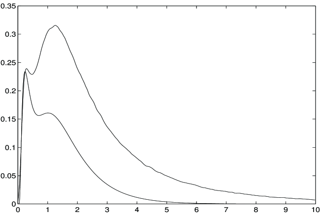
Figure 1: FPT density $h_{k}(\beta,t\,|\,x_{0})$ and its lower bound for exponentially distributed alternating times, with rates $\lambda_{1}=1/2$ and $\lambda_{2}=2$, and $\mu_{1}=1$, $\mu_{2}=-1$, $\sigma_{1}^{2}=1$, $\sigma_{2}^{2}=10$, $\beta=3$, $x_{0}=0$ and $k=2$.

We point out that the role of alternating processes governed by exponentially-distributed alternating times has already been outlined in the biomathematical literature. For instance, as mentioned in Stadje (1987), some experimental studies suggest that the motion of certain micro-organisms can be approximated by trajectories that change directions at exponentially distributed random times. Another example of great biological interest, already referred to in Section 1, is found in Kitamura et al. (1999), where it is experimentally shown that the dwell times between consecutive jumps in the rising phase of myosin movements along actin filament during muscle contraction are exponentially distributed. Furthermore, aiming to describe the firing activity of a neuronal model subject to alternating input, a Wiener process with drift alternating at exponentially distributed times was recently studied by Buonocore et al. (2001). These are paradigmatic examples that lead one to focus attention on Brownian motion with alternating infinitesimal moments in the special case when the alternating times are exponentially distributed. Hereafter we show that in such a case the FPT pdf through constant boundaries for process (2) is not necessarily unimodal, quite differently from the case of the Wiener process that leads to rigorously unimodal densities. Figure 1 shows a bimodal estimate of FPT pdf $h_{2}(3,t\,|\,0)$ obtained via our simulation procedure, together with the corresponding lower bound provided in (14), under the assumption that the alternating random times are exponentially distributed, with $\overline{F}_{U}(t)=e^{-t/2}$ and $\overline{F}_{D}(t)=e^{-2\,t}$, $t\geq 0$.

5 Applications

Hereafter, we shall indicate two different applications of the foregoing results and simulation procedure. The first application is of interest to environmental sciences. Aiming to theoretically construct a link between the intermittence of rainfall and the dynamics of moisture processes, in Freidlin and Pavlopoulos (1997) a stochastic model has been proposed in which the temporal evolution of the moisture content in a given atmospheric column is described by a stochastic process. This consists of the alternation of two Wiener processes with drifts of opposite signs and unequal infinitesimal variances, the alternation taking place when an upper saturation threshold or a lower dehydration threshold is reached. As a possible alternative model, we select process (2) to describe the temporal evolution of the moisture content. Differently from Freidlin and Pavlopoulos (1997), in our model the alternation between two different regimes does not occur at the thresholds’ reaching times, but at the occurrence of random times (1). However, in order to keep a similarity between the alternating mechanism of those two models, we assume that the inter-swithching times are distributed as in Freidlin and Pavlopoulos (1997). Hence, random variables $U_{1},U_{2},\ldots$ and $D_{1},D_{2},\ldots$ are now assumed to have inverse Gaussian pdf’s

$$f_{U}(x)=\sqrt{l_{1}\over 2\pi x^{3}}\,\exp\left\{-{l_{1}(x-m_{1})^{2}\over 2m^{2}_{1}x}\right\},\qquad f_{D}(x)=\sqrt{l_{2}\over 2\pi x^{3}}\,\exp\left\{-{l_{2}(x-m_{2})^{2}\over 2m^{2}_{2}x}\right\},$$ (33)

for $x>0$. The removal of the thresholds is acceptable because, according to Freidlin and Pavlopoulos (1997), no empirical verification is available for their existence. Furthermore, it is also reasonable to assume that the alternating of dry and wet durations is regulated by a mechanism somewhat looser than that including the presence of precisely specified saturation and dehydration thresholds.

As study case we refer to the measurements performed within the TOGA-COARE (Tropical Ocean Global Atmosphere – Coupled Ocean-Atmosphere Response Experiment) and reported in Freidlin and Pavlopoulos (1997). Making use of the estimates obtained by these authors via the method of moments, we are led to the following values for the parameters appearing in (33) and for the alternating infinitesimal moments of $\{X(t)\}$:

$$\begin{array}[]{llll}l_{1}=0.7518,&m_{1}=1.4215,&l_{2}=0.5073,&m_{2}=1.0476,\\ \mu_{1}=0.2313,&\sigma_{1}=0.3792,&\mu_{2}=-0.3139,&\sigma_{2}=0.4616.\end{array}$$ (34)

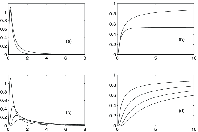
Figure 2: (a) FPT density $h_{k}(\beta,t\,|\,x_{0})$ and its lower bound for inverse Gaussian distributed alternating times, with parameters given in (34), $k=1$, $x_{0}=0$ and $\beta=0.3$; (b) the corresponding distribution function $H_{k}(\beta,t\,|\,x_{0})$ and its lower bound; (c) FPT densities as in (a) with (from top to bottom near the origin) $\beta=0.3$, $0.5$, $0.7$, $0.9$; (d) the corresponding distribution functions.

Since the magnitude of negative drift exceeds that of positive drift, a negative net displacement is obtained. Figure 2 shows the estimates of FPT pdf $h_{k}(\beta,t\,|\,x_{0})$ and of the corresponding cdf $H_{k}(\beta,t\,|\,x_{0})$ obtained by means of our simulation procedure, as well as the corresponding lower bounds provided in Section 3. Computations make use of densities (33) and of the estimates (34) of parameters. The simulation of the inverse Gaussian distributed random times has been performed by the method of Michael et al. (1976).

We now come to an application in mathematical finance. As is well known, one of stochastic processes often used to describe the time course of the price $S(t)$ of risky assets is the geometric Brownian motion

$$S(t)=s_{0}\,\exp\{\mu\,t+\sigma\,B(t)\},\qquad t\geq 0.$$

An extension of this model is based on the assumption that parameters $\mu$ and $\sigma$ alternate between two values, with variations occurring randomly in time according to an alternating renewal process. Such alternation is meant to be responsible for the floating behavior of prices, which are often subject to alternating periods of growing and decreasing trends, though maintaining their high level of stochasticity. We thus refer to a continuous-time stochastic process $\{S(t),t\geq 0\}$ with state-space $(0,+\infty)$ defined as

$$S(t)\!\!\! = \!\!\!s_{0}\,\exp\{X(t)-x_{0}\}$$ (35)

$$= \!\!\!s_{0}\,\exp\left\{\int_{0}^{t}\mu(\tau)\,{\rm d}\tau+\sigma(t)\,B(t)\right\},\qquad t\geq 0,$$

with $s_{0}>0$, and where $X(t)$ is defined in (2), and $\mu(t)$ and $\sigma(t)$ are given in (3). Model (35) characterizes a growing trend when $\delta(t)=1$, i.e. $\mu(t)=\mu_{1}\geq 0$ and $\sigma(t)=\sigma_{1}$, and a decreasing trend when $\delta(t)=2$, i.e. $\mu(t)=\mu_{2}\leq 0$ and $\sigma(t)=\sigma_{2}$. The initial trend is determined by $\delta(0)\in\{1,2\}$.

To come to the FPT problem through the boundary $\beta>s_{0}$, let

$$T_{k}^{S}:=\inf\{t>0:S(t)>\beta\},\qquad S(0)=s_{0},\;\delta(0)=k\in\{1,2\}.$$

Hence, $T_{k}^{S}$ describes the first time when price $S(t)$ reaches the level $\beta$ from below. This is of interest in mathematical finance when $\beta$ may represents some critical threshold for price $S(t)$. We denote by $h_{k}^{S}(\beta,t\,|\,s_{0})$ and by $H_{k}^{S}(\beta,t\,|\,s_{0})$ the pdf and the cdf of $T_{k}^{S}$, respectively. Recalling (5) and (6), from (35) and the independence of the increments of $\{X(t)\}$ one can see that

$$h_{k}^{S}(\beta,t\,|\,s_{0})=h_{k}\left(\ln{\beta\over s_{0}},t\,\Bigg{|}\,0\right),\qquad H_{k}^{S}(\beta,t\,|\,s_{0})=H_{k}\left(\ln{\beta\over s_{0}},t\,\Bigg{|}\,0\right),\qquad t>0.$$ (36)

Hence, $h_{k}^{S}$ and $H_{k}^{S}$ can be estimated by resorting to the method described in Section 4 for $h_{k}$ and $H_{k}$, whereas bounds for $h_{k}^{S}$ and $H_{k}^{S}$ can be obtained by means of Eq. (36) and Theorems 3.1 and 3.3.

In order to include in model (35) the occurrence of periods of alternating trends characterized by heavy-tailed distributions, we assume that the random times $U_{n}$, $D_{n}$ have respectively generalized Pareto distribution

$$F_{U}(x)=1-\left(1+\xi_{1}\,\frac{x}{\eta_{1}}\right)^{-1/\xi_{1}},\qquad F_{D}(x)=1-\left(1+\xi_{2}\,\frac{x}{\eta_{2}}\right)^{-1/\xi_{2}},\qquad x>0,$$ (37)

with $\xi_{k}>0$ and $\eta_{k}>0$, $k=1,2$. This is quite reasonable, since such distribution is known to play a relevant role in various applied fields such as those related to insurance, finance, telecommunication traffic, queueing, in which (see, for instance, Mikosch and Nagaev, 1998, and Greiner et al., 1999) measurements of time series show large degrees of variability in the arrival rates, and long-range dependence effects.

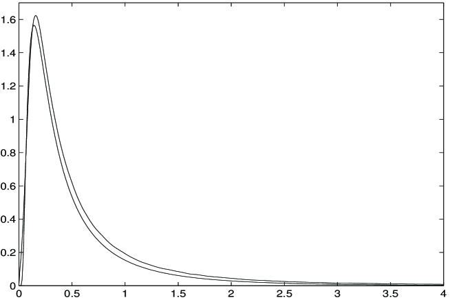
Figure 3: An example of estimated FPT density $h_{1}^{S}(2,t\,|\,1)$ and of its lower bound. Here process (35) is characterized by $\mu_{1}=1$, $\mu_{2}=-1$ and $\sigma_{1}=\sigma_{2}=1$. The alternating times occur according to a generalized Pareto distribution (37), with $\xi_{1}=1$, $\eta_{1}=2$, $\xi_{2}=3$ and $\eta_{2}=4$.

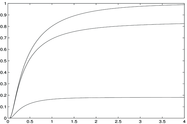
Figure 4: Cumulative distribution function $H_{1}^{S}(2,t\,|\,1)$ and its bounds under the assumptions of Fig. 3. The upper bound is obtained from (26), holding for $\sigma_{1}=\sigma_{2}$.

An example of estimate of FPT pdf $h_{1}^{S}(2,t\,|\,s_{0})$ and of its lower bound, obtained by means of our simulation procedure is provided in Figure 3, whereas the corresponding cdf $H_{1}^{S}(2,t\,|\,s_{0})$ and its lower and upper bounds are shown in Figure 4.

Appendix

This Appendix is devoted to a thorough description of the probability arguments underlying some steps of the procedure referred to in Section 4 to simulate the random variables having pdf’s (30) and (31).

A1. Simulation when first passage has already occurred

Based on the Von Neumann acceptance-rejection (VNAR) method (see for instance Ross, 1989) the following procedure simulates the generation of a pseudo-random number from the r.v. with pdf $f_{1}(\theta)$ given in (30):

$$\begin{array}[]{l}\hbox{\bf Procedure}\\ \hbox{{Step 1.}$\;$ evaluate the maximum $m:=f_{1}(\theta_{m})$ of the pdf~{}{\rm(\ref{equation:14})};}\\ \hbox{{Step 2.}$\;$ if $1/(m\tau)\leq\varepsilon_{2}$ then $\theta:=\theta_{m}$ and goto {Step 5};}\\ \hbox{{Step 3.}$\;$ generate two uniform independent pseudo-random numbers $x$ in $(0,\tau)$ and $y$ in $(0,m)$;}\\ \hbox{{Step 4.}$\;$ if $y\leq f_{1}(x)$ then $\theta:=x$, else goto {Step 3};}\\ \hbox{{Step 5.}$\;$ return($\theta$).}\end{array}$$

Concerning Step 1, we point out that density (30) is limited by the maximum $m=f_{1}(\theta_{m})$ located at $\theta_{m}=\min\{\tau,c_{m}\}$, where

$$c_{m}=\cases{\displaystyle{-3\sigma^{2}_{k}+\sqrt{9\sigma^{4}_{k}+4\mu_{k}^{2}(\beta-x)^{2}}\over 2\mu_{k}^{2}}&if $\mu_{k}\neq 0$,\cr\hfill\cr\displaystyle{(\beta-x)^{2}\over 3\sigma^{2}_{k}}&if $\mu_{k}=0$.}$$

Then, $m\tau\geq\int_{0}^{\tau}f_{1}(\theta)\,d\theta=1$ since $m\geq f_{1}(\theta)$ for all $\theta\in(0,\tau)$. Hence, by Step 1 the maximum $m:=f_{1}(\theta_{m})$ of the pdf (30) is evaluated, to yield $\theta_{m}$ as output if $1/(m\tau)\leq\varepsilon_{2}$, where $\varepsilon_{2}$ is a preassigned tolerance parameter. If $1/(m\tau)>\varepsilon_{2}$, by Step 3 two uniform independent pseudo-random numbers $x$ in $(0,\tau)$ and $y$ in $(0,m)$ are being generated as long as there results $y\leq f_{1}(x)$. At such stage, the corresponding value of $x$ is yielded as output (Step 4). We point out that Step 3 and Step 4 rely on the following proposition whose straightforward proof is omitted.

Proposition 1

If $W_{k}(0)=x$, for all $\theta\in(0,\tau)$ there holds

$$\mathop{\rm P}\left(T_{k}^{W}\leq\theta\,\Big{|}\,T_{k}^{W}\leq\tau\right)=\mathop{\rm P}[X\leq\theta\,|\,Y\leq f_{1}(X)],$$

where $X$ is uniformly distributed in $(0,\tau)$, $Y$ is uniformly distributed in $(0,m)$, $X$ and $Y$ are independent, and $m$ is the maximum over $(0,\tau)$ of the pdf $f_{1}(\theta)$ given in (30).

A2. Simulation when first passage has not yet occurred

In the procedure listed below, again a classical VNAR method is implemented in order to construct a pseudo-random number from the r.v. having pdf (31):

$$\begin{array}[]{l}\hbox{\bf Procedure}\\ \hbox{{Step 1.}$\;$ by {\bf Subroutine} generate a pseudo-random number $z$ from the r.v.\ with pdf}\\ \hbox{\qquad$f_{3}(z)$; \quad[see Eq.~{}{\rm(\ref{equation:16})}]}\\ \hbox{{Step 2.}$\;$ generate an uniform pseudo-random number $u$ in $(0,1)$;}\\ \hbox{{Step 3.}$\;$ if $u\leq\ell(z)$ then $x:=z$, else goto {Step 1};}\\ \hbox{{Step 4.}$\;$ return($x$).}\\ \hbox{{\bf Subroutine} (simulates a truncated Gaussian density)}\\ \hbox{{Step S1.}$\;$ $q:=1-\Phi\left({\beta-x-\mu_{k}\,\tau\over\sigma_{k}\,\sqrt{\tau}}\right)$;}\\ \hbox{{Step S2.}$\;$ if $q<\varepsilon_{3}$ then $\{$ generate a standard normal pseudo-random number $n$;}\\ \hbox{\qquad$w:=n$ and goto {Step~{}S7} $\}$;}\\ \hbox{{Step S3.}$\;$ generate two uniform independent pseudo-random numbers $u$ and $v$ in $(0,1)$;}\\ \hbox{{Step S4.}$\;$ $y:=\log v+{\beta-x-\mu_{k}\,\tau\over\sigma_{k}\sqrt{\tau}}$;}\\ \hbox{{Step S5.}$\;$ if $u\geq\xi(y)$ then goto {Step~{}S3}; \quad[see Eq.~{}{\rm(\ref{equation:19})}] }\\ \hbox{{Step S6.}$\;$ $w:=y$;}\\ \hbox{{Step S7.}$\;$ $z:=x+\mu_{k}\,\tau+w\,\sigma_{k}\,\sqrt{\tau}$;}\\ \hbox{{Step S8.}$\;$ return($z$).}\end{array}$$

We point out that use of VNAR method requires that the density (31) to be simulated be factorized as follows:

$$f_{2}(z)=C\,f_{3}(z)\,\ell(z),\qquad-\infty<z<\beta,$$ (38)

where $C=[1-G_{k}(\beta,\tau\,|\,x)]^{-1}$,

$$f_{3}(z)={1\over\sqrt{2\pi\sigma^{2}_{k}\tau}}\,\exp\left\{-{(z-x-\mu_{k}\tau)^{2}\over 2\sigma^{2}_{k}\tau}\right\}{1\over\Phi\left({\beta-x-\mu_{k}\tau\over\sigma_{k}\sqrt{\tau}}\right)},\qquad-\infty<z<\beta,$$ (39)

and

$$\ell(z)=\Phi\left({\beta-x-\mu_{k}\tau\over\sigma_{k}\sqrt{\tau}}\right)\left[1-\exp\left\{-{2\over\sigma^{2}_{k}\tau}\,(\beta-z)\,(\beta-x)\right\}\right],\qquad-\infty<z<\beta.$$ (40)

Note that factorization (39) is made possible by virtue of (11). Step 1 of the procedure can thus be performed.

We note that $C\geq 1$, $f_{3}(z)$ is the truncation over $(-\infty,\beta)$ of a Gaussian density with mean $x+\mu_{k}\tau$ and variance $\sigma^{2}_{k}\tau$, while $\ell(z)\in[0,1]$ for all $z\in(-\infty,\beta)$. The implemented VNAR method requires the generation by a suitable subroutine of a pseudo-random number from the r.v. $Z$ having pdf (39) as summarized in Steps S1-S8. Step S7 gives $Z$ as output when $U\leq\ell(Z)$, where $U$ is an uniform pseudo-random number in $(0,1)$. We point out that the described procedure makes use of the following

Proposition 2

For all $z\in(-\infty,\beta)$, we have:

$$\int_{-\infty}^{z}f_{2}(y)\,dy=\mathop{\rm P}\left[Z\leq z\,|\,U\leq\ell(Z)\right],$$

where $U$ and $Z$ are independent r.v.’s that are distributed uniformly in $(0,1)$ and according to pdf (39), respectively.

The above subroutine is based on the following considerations. First of all, the subroutine generates a pseudo-random number $z$ from the r.v. with pdf $f_{3}(z)$ given in Eq. (39). We note that if (39) is the pdf of $Z$, then

$$W=\frac{Z-x-\mu_{k}\tau}{\sigma_{k}\sqrt{\tau}}$$ (41)

is a truncated standard normal r.v. possessing pdf

$$f_{W}(z)=\displaystyle{\frac{1}{\sqrt{2\pi}}}\exp\left\{-\frac{z^{2}}{2}\right\}\frac{1}{\Phi\left(\frac{\beta-x-\mu_{k}\,\tau}{\sigma_{k}\,\sqrt{\tau}}\right)},\qquad z<\frac{\beta-x-\mu_{k}\,\tau}{\sigma_{k}\,\sqrt{\tau}}.$$ (42)

Via (41) the subroutine thus generates a pseudo-random number from $Z$ by sampling a pseudo-random number from $W$. To this purpose, for a preassigned tolerance parameter $\varepsilon_{3}$, if

$$1-\Phi\left(\frac{\beta-x-\mu_{k}\,\tau}{\sigma_{k}\,\sqrt{\tau}}\right)<\varepsilon_{3},$$ (43)

then the distribution of $W$ is approximated by a standard normal distribution. Therefore, a generation of a value for $W$ is performed by implementing any classical generator of standard gaussian r.v. (see Step S2). If (43) is not fulfilled, the following classical VNAR method is employed (see Steps S3-S6). Consider the r.v. $Y$, having pdf

$$f_{4}(y)=\cases{\exp\left\{y-\displaystyle{\beta-x-\mu_{k}\,\tau\over\sigma_{k}\,\sqrt{\tau}}\right\}&if $y<\displaystyle{\beta-x-\mu_{k}\,\tau\over\sigma_{k}\,\sqrt{\tau}}$,\\ \hfill\cr 0&otherwise,}$$ (44)

with $k\in\{1,2\}$, $x,\beta\in\vbox{\hbox to8.9pt{I\hskip-2.1ptR\hfil}}$, $x\leq\beta$ and $\tau>0$. Then, the pdf given in (42) can be expressed as

$$f_{W}(z)=D\,f_{4}(z)\,\xi(z),\qquad z<\frac{\beta-x-\mu_{k}\,\tau}{\sigma_{k}\,\sqrt{\tau}},$$

where

$$D=\frac{1}{\Phi\left(\frac{\beta-x-\mu_{k}\,\tau}{\sigma_{k}\,\sqrt{\tau}}\right)}\exp\left\{\frac{\beta-x-\mu_{k}\,\tau}{\sigma_{k}\sqrt{\tau}}+4\right\}$$

and

$$\xi(z)=\frac{1}{\sqrt{2\pi}}\,\exp\left\{-\frac{z^{2}+2\,z+8}{2}\right\},$$ (45)

with $0\leq\xi(z)\leq 1$. Note that $D\geq 1$ since

$$\frac{\beta-x-\mu_{k}\,\tau}{\sigma_{k}\,\sqrt{\tau}}+4>0.$$

A pseudo-random number from $Y$ is generated (Step S4) by using the inversion method of cdf’s. We thus have

$$Y=\log U_{2}+\frac{\beta-x-\mu_{k}\,\tau}{\sigma_{k}\sqrt{\tau}}\qquad\Longleftrightarrow\qquad U_{2}=e^{Y-\displaystyle{\frac{\beta-x-\mu_{k}\,\tau}{\sigma_{k}\sqrt{\tau}}}}=F_{Y}(Y),$$

where $F_{Y}(\cdot)$ is the cdf of $Y$. Then, (Step S5), the subroutine samples a value for $W$ as long as

$$u\leq\xi\left(\log v+\frac{\beta-x-\mu_{k}\,\tau}{\sigma_{k}\sqrt{\tau}}\right),$$

with $u$ and $v$ pseudo-random numbers in $(0,1)$ and where $\xi(\cdot)$ is given in  (45). The theoretical justification is provided by the following proposition, whose straightforward proof is omitted.

Proposition 3

For all $z<(\beta-x-\mu_{k}\,\tau)/(\sigma_{k}\,\sqrt{\tau})$ it is

$$\int_{-\infty}^{z}f_{W}(y)\,dy=\mathop{\rm P}[Y<z\,|\,U<\xi(Y)],$$

where $f_{W}(y)$ is the pdf given in (42), $U$ and $Y$ are independent r.v.’s such that $U$ is uniformly distributed in $(0,1)$ and $Y$ has pdf (44), and where $\xi(\cdot)$ is defined in (45).

The theoretical justification of the simulation procedure is thus completed.

Acknowledgments

We thank an anonymous reviewer for his criticism on a previous version of this paper. This work has been performed within a joint cooperation agreement between Japan Science and Technology Corporation (JST) and Università di Napoli Federico II, under partial support by MIUR (cofin 2003) and by G.N.C.S. (INdAM).

References

A. Buonocore, A. Di Crescenzo and E. Di Nardo, “Input-output behavior of a model neuron with alternating drift,” BioSystems vol. 67 pp. 27–34, 2002.

A. Buonocore, A.G. Nobile and L.M. Ricciardi, “A new integral equation for the evaluation of first-passage-time probability densities,” Adv. Appl. Prob. vol. 27 pp. 102–114, 1987.

D. Cyranoski, “Swimming against the tide,” Nature vol. 408 pp. 764–766, 2000.

A. Di Crescenzo, “On Brownian motions with alternating drifts,” in Cybernetics and Systems 2000 (Trappl R. ed.), Vienna, Austria, 2000, pp. 324–329.

E. Di Nardo, A.G. Nobile, E. Pirozzi and L.M. Ricciardi, “A computational approach to first-passage-time problems for Gauss-Markov processes,” Adv. Appl. Prob. vol. 33 pp. 453–482, 2001.

M. Freidlin and H. Pavlopoulos, “On a stochastic model for moisture budget in an Eulerian atmospheric column,” Environmetrics vol. 8 pp. 425–440, 1997.

A. Giorno, A.G. Nobile and L.M. Ricciardi, “On the evaluation of first-passage-time probability densities via nonsingular equations,” Adv. Appl. Prob. vol. 21 pp. 20–36, 1989.

M. Greiner, M. Jobmann and C. Klüppelberg, “Telecommunication traffic, queueing models, and subexponential distributions,” Queueing Systems vol. 33 pp. 125–152, 1999.

K. Kitamura, M. Tokunaga, A. Hikikoshi Iwane and T. Yanagida, “A single myosin head moves along an actin filament with regular steps of 5.3 nanometres,” Nature vol. 397 pp. 129–134, 1999.

J.R. Michael, W.R. Schucany and R.W. Haas, “Generating random variates using transformations with multiple roots,” The American Statistician vol. 30 pp. 88–90, 1976.

T. Mikosch and A.V. Nagaev, “Large deviations of heavy-tailed sums with applications in insurance,” Extremes vol. 1 pp. 81–110, 1998.

L.M. Ricciardi, A. Di Crescenzo, V. Giorno and A.G. Nobile, “An outline of theoretical and algorithmic approaches to first passage time problems with applications to biological modeling,” Mathematica Japonica vol. 50 pp. 247–322, 1999.

S. Ross, Introduction to Probability Models, Fourth Edition, Academic Press: Boston, 1989.

M. Shaked and J.G. Shanthikumar, Stochastic Orders and Their Applications, Academic Press: San Diego, 1994.

B.W. Silverman, Density Estimation for Statistics and Data Analysis, Chapman and Hall: London, 1986.