Mapping the Sun’s upper photosphere with artificial neural networks

We have developed an inversion procedure designed for high-resolution solar spectro-polarimeters, such as Hinode/SP or DKIST/ViSP. The procedure is based on artificial neural networks trained with profiles generated from random atmospheric stratifications for a high generalization capability. When applied to Hinode data we find a hot fine-scale network structure whose morphology changes with height. In the middle layers this network resembles what is observed in G-band filtergrams but it is not identical. Surprisingly, the temperature enhancements in the middle and upper photosphere have a reversed pattern. Hot pixels in the middle photosphere, possibly associated to small-scale magnetic elements, appear cool at the $\log\tau_{500}$=$-3$ and $-4$ level, and viceversa. Finally, we find hot arcs on the limb side of magnetic pores, which we interpret as the first direct observational evidence of the ”hot wall” effect in temperature.

1 Introduction

Inversion techniques allow us to retrieve information encoded in spectral lines about the atmospheres where they form. A wide variety of strategies have been employed for decades in solar physics to interpret spectroscopic and spectropolarimetric observations (see e.g. the reviews by del Toro Iniesta & Ruiz Cobo 2016; Bellot Rubio 2006; Socas-Navarro 2001). Most applications are based on the least-squares fitting of the observed spectral lines with synthetic profiles, which are computed from model atmospheres whose parameters are iteratively adjusted until a satisfactory fit is attained. However, advances in instrumentation are driving an increasing interest in the exploration of alternative methods. Two-dimensional spectropolarimetry is now very common and fast growing data rates motivate the exploration of new algorithms that have the potential of being faster and/or more robust for systematic application.

Artificial neural networks (ANNs) offer a promising new approach for many purposes where profile fitting is inadequate because one needs a faster or a more robust performance. The first applications of ANNs in solar physics are almost 20 years old, dating back to Carroll & Staude (2001) and Socas-Navarro (2002). However, while those first efforts produced encouraging results, ANN inversions were not immediately adopted by the community, for two reasons mainly. First, disentangling the magnetic filling factor from the intrinsic field strength has proven extremely challenging, as noted since those early works (Socas-Navarro 2003). The magnetic field tends to exhibit small-scale structures in the solar photosphere. In arc-second resolution observations, it is common to find pixels where the magnetic field occupies less than 10% of the resolution element. This area fraction is referred to as the filling factor and it introduces an important complication for ANN inversions. Second, a more practical issue is the complexity involved in the coding of algorithms for the training of an ANN model.

Those early problems have been largely resolved in recent years, leading to a renewed interest in ANNs (e.g., Liu et al. 2020; Guo et al. 2020; Díaz Baso & Asensio Ramos 2018; Asensio Ramos & Díaz Baso 2019; Felipe & Asensio Ramos 2019; Milić & Gafeira 2020). Current (and upcoming) instrumentation are delivering very high resolution observations, mitigating the filling factor problem. Furthermore, there has been a tremendous development in the field of deep learning and many sophisticated tools have been made publicly available to simplify the problem of building and training ANNs (e.g., Abadi et al. 2015; Paszke et al. 2019).

In this paper we use a relatively simple ANN model and take a different approach to previous work for the training strategy. Instead of using a simulation snapshot as the starting point for a training set, as in Asensio Ramos & Díaz Baso (2019) or Milić & Gafeira (2020), we create a database of profiles from random stratifications of the relevant parameters. This provides a wide coverage of the parameter space and guarantees that the ANN is not specialized on any particular scenario. Unlike Asensio Ramos & Díaz Baso (2019), whose ANN performs a full inversion of the entire 2D field at once, this ANN works on each pixel independently. In that regard, it is more similar to a traditional inversion technique.

We created two different ANNs, one to invert photospheric observations from DKIST/ViSP (Daniel K Inouye Solar Telescope/Visible Spectro-Polarimeter, see Rimmele et al. 2020) and the other one for the Hinode satellite’s SOT/SP (Solar Optical Telescope/Spectro-Polarimeter). DKIST/ViSP data are not yet available so we focus here on the analysis of the Hinode inversions. After testing the procedure with synthetic data and previous inversions of real observations, we applied it to Hinode observations of active regions. In this manner we obtained datacubes with a fairly unique combination of high spatial resolution, large field of view and depth-dependent temperatures. These maps show a fine hot network in active regions, particularly around sunspots and pores.

We find some surprising results in this application, such as an anticorrelation between hot pixels in middle and upper layers. Also, the inversions reveal a series of hot arcs running along the limb side of pores in the observed regions. We interpret these arcs as the first direct observation of the ”hot wall” effect, a prediction of fluxtube models since the work of Spruit (1976) which had not been directly observed thus far.

2 The ANN model and training set

All the calculations presented in this paper were produced with relatively standard computer hardware. We employed a Linux workstation powered by eight 3·GHz Intel Xeon cores. The system is equipped with a GTX 1080 GPU that handles most of the ANN-related processing. Our ANN model and codes are publicly available in a repository.

The ANN is created and trained using PyTorch (Paszke et al. 2019). It is a simple multilayer perceptron with six hidden layers between the input and output layers. Each hidden layer comprises 300 neurons. The input layer has a number of neurons that matches the number of spectral pixels in a given profile (175 for DKIST/ViSP and 112 for Hinode SOT/SP). The output layer has 9 neurons, which correspond to the output parameters that we wish to retrieve. These parameters are: 5 temperatures at different heights, 3 components of the magnetic field vector and a single-valued line-of-sight velocity. In all cases, the activation function chosen is a leaky ReLU (Maas et al. 2013). The entire training procedure takes a few hours on our hardware described above.

For the training and validation sets we compute one million synthetic profiles from randomized model atmospheres. A thousand models and profiles are taken as the validation set and the rest are used for training. These models are obtained as random variations from four different reference atmospheres, namely: HSRA (Gingerich et al. 1971), VAL-C (Vernazza et al. 1981), FAL-C (Fontenla et al. 1993) and the sunspot model M of Maltby et al. (1986). We provide here a description of the randomization procedure in some detail because the construction of this database is critical for the ability of the ANN to perform adequately when faced with real observations and to exhibit good generalization properties.

For each relevant parameter, we take the stratification in the reference atmosphere and add a depth-dependent perturbation to it. The perturbation is constructed by assigning values to certain layers and then interpolating in depth. In the case of temperature, the parameter to which spectral lines are most sensitive, we start by creating a perturbation at four layers. These layers are not necessarily the same heights that the ANN will retrieve. They are equispaced in the logarithm of continuum optical depth at 500 nm ($\log\tau_{500}$) and their actual location is different for the four reference atmospheres. The perturbations at these four points are drawn from a Gaussian distribution with a 1,500 K standard deviation. From these four values, the depth-dependent perturbation is interpolated to the entire grid and added to the reference model. With the new thermal stratification, the model is set in hydrostatic equilibrium and the equation of state is solved to compute plasma densities, ionization fractions, relevant molecules and electron densities.

For the magnetic field, we have that $B_{z}$ (the line-of-sight component) is linear in $\log\tau_{500}$, whereas $B_{x}$ and $B_{y}$ (the transverse components) are constant with height. $B_{z}$ is defined by $B_{z}(0)$, its value at $\log\tau_{500}$ $=0$, and its gradient. We construct three possible scenarios with weak, strong and extreme fields, having probabilities of 45%, 45% and 10% respectively. The field strength $B_{z}(0)$ takes values from a uniform distribution with a width of 500, 2000 and 6000 $G$ for the weak, strong and extreme fields, respectively. The sign for each field component is randomly set to $\pm 1$ except for $B_{x}$, which is always taken as positive. Since the Zeeman effect has a 180-degree ambiguity in the transverse component of the field, we restrict our solutions to the subspace with positive $B_{x}$. The $B_{z}$ gradient is set to either 0 or a random value, with a 50% probability. The random value is taken from a uniform probability distribution between -150 and 150 $G$ per unit in $\log\tau_{500}$.

The filling factor ($\alpha$) is set to 1 in 50% of the models. The rest have a uniform distribution between 0.1 and 1. In addition to the filling factor, we consider a fixed amount of stray light in the instrument by adding an average quiet Sun profile to Stokes I. The amount of stray light is fixed to 10%, which is a typical value for spectrographs.

This training set was built with the purpose of covering a sufficiently wide range of profiles for the ANN to work with all possible observations of the solar photosphere in the 630 nm spectral window observed by Hinode. The statistical distribution of our random atmospheres is not necessarily optimal. We relied on past experience and numerical experimentation to determine a suitable set. A systematic analysis is beyond the scope of this work.

We used NICOLE (Socas-Navarro et al. 2015) to compute synthetic Stokes profiles for the entire set of one million random models in the database. The synthesis parameters for one of the training sets were defined to mimic Hinode/SP observations. DKIST/ViSP will also feature a preset mode to observe the same 630 nm window so we produced another similar set of profiles simulating those observations in anticipation of its science operations. Both training sets are publicly available in the repository mentioned above.

Figure 1: Comparison of inversions of a Hinode map performed with NICOLE (left) and our ANN (right).

The Stokes profiles are fed as inputs to the ANN. For the outputs, we extract a set of 9 parameters from the random model atmospheres in the database. These parameters are: five temperatures ($T_{0}$, …, $T_{4}$), extracted at optical depths $\log\tau_{500}$= $0$,…,$-4$, a bulk Doppler velocity ($v_{z}$) and the three components of the pixel-averaged magnetic field ($F_{x}$, $F_{y}$, $F_{z}$, where $F_{i}=\alpha B_{i}$ for $i=x,y,z$). We do not aim here at disentangling the filling factor $\alpha$ from the intrinsic magnetic field strength ($B_{i}$) in the magnetic element. We seek to retrieve the magnetic flux density ($F$) in the resolution element, which simplifies the problem.

Figure 2: Comparison of inversions of a Hinode map performed with NICOLE (left) and our ANN (right). Positive (negative) velocities are directed downards (upwards). Positive (negative) magnetic polarity represents fields pointing up (down) from the solar surface.

3 Comparisons with other inversions

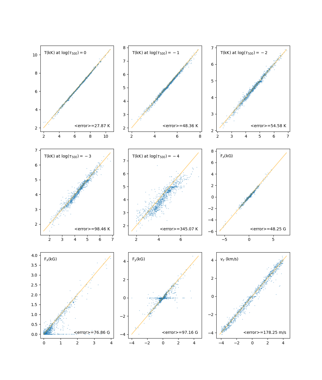
After successfully training the ANN and observing a good recovery of the validation set (see Figure 3), we tested it with real observations. As noted in previous work (Socas-Navarro 2005), a good performance with the validation set composed of synthetic observations does not guarantee a good operation with real data.

Figure 3: Tests of the ANN performance with the validation set. Abscissas are the ”true” values and ordinates are the ANN outputs. Each plot shows the average (median) error in the recovery of that parameter.

Ideally, one would like to have inversions of Hinode/SP data to compare with our ANN. Unfortunately, there are very few inversions of Hinode/SP maps that yield the height stratification. The standard pipeline includes an inversion carried out by the instrument team with the MERLIN code (Lites et al. 2007), which is based on the Milne-Eddington approximation and therefore does not provide information on the height dependence of any physical quantities. One of the few inversions with the height stratification existing in the literature is that of Socas-Navarro (2011) using NICOLE (later refined in Socas-Navarro 2015).

We took the same Hinode/SP observations used for the NICOLE inversions and processed them with our ANN. The NICOLE inversions took about 5 hours on a dedicated parallel run over the eight cores of our workstation. The ANN inversion was completed in half a second.

Figure 4: Comparison of inversions of a Hinode map (map1) performed with MERLIN (left column) and our ANN (center). Scatter plots are shown in the right column. Positive (negative) magnetic polarity represents fields pointing up (down) from the solar surface.

Figure 5: Comparison of inversions of a Hinode map (map2) performed with MERLIN (left column) and our ANN (center). Scatter plots are shown in the right column. Positive (negative) magnetic polarity represents fields pointing up (down) from the solar surface.

An additional postprocessing renormalization was applied on each ANN temperature output, so that the average value would match that of the NICOLE inversions. This is done to remove (at least to first order) some small residuals that arise in the application to real data.

We do not find these residuals in the validation tests so they must be due to systematic differences between our synthetic training set and the real observations, such as observation artifacts, differences in the PSF or an inaccurate estimate of the stray light used in the synthesis. A detailed analysis of these residuals is beyond the scope of this paper but for our purposes here, this simple renormalization (the same for all observations) resolves the issue.

The normalization factors for $T_{0}$,…,$T_{4}$ are 0.90,1.26,1.29,1.44 and 1.60, respectively. The growing trend of these factors indicates that the ANN produces models that are, on average, steeper than those obtained with NICOLE. The synthesis tests presented below demonstrate that the model atmospheres obtained in this manner produce spectral profiles very similar to the observations. For the magnetic field (see below), this calibration yields a factor of 0.7 in all three components. We incorporate this normalization factor in all subsequent inversions.

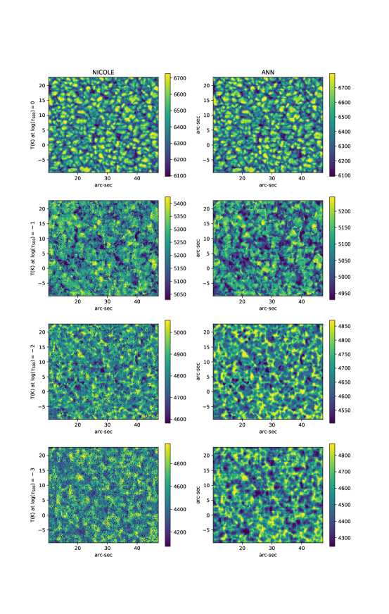
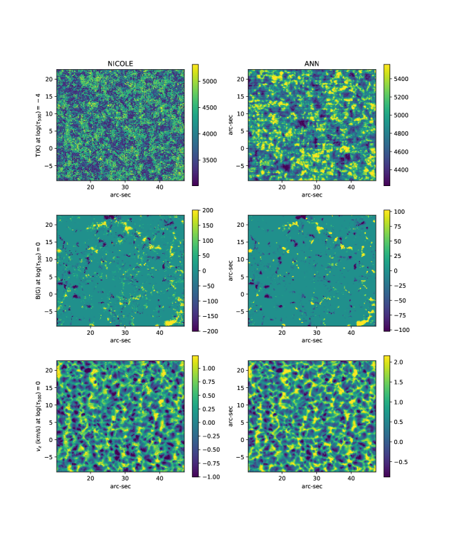
A comparison of the maps produced by the ANN and those from NICOLE (the 2015 version) is presented in Figs 1 and 2. The similarity between the spatial structures in the images obtained with both techniques is remarkable. The NICOLE inversions are much more noisy, especially in the higher layers. ANNs are known to have good noise filtering properties. In this case, most of the noise in the NICOLE data is ”inversion noise” produced by the specific $\chi^{2}$ fitting procedure that seeks the best fit to the entire line profile. The upper layers are probed only by the core of the spectral lines. Since the core occupies very few pixels in the spectral profile, there is very little information about those upper layers. For very similar profiles, the $\chi^{2}$ minimization might reach slightly different solution where the core is fitted with more or less accuracy, perhaps compensating it with a better fit to other spectral regions. The end result is a pixel-to-pixel variation that becomes more important in those layers where the profile is less sensitive. This problem could be mitigated by fine-tuning the weights, giving more weight to the pixels that carry the relevant information. However, different layers would require a different optimization.

The ANN, on the other hand, ”learns” what are the optimal spectral points that it needs to focus on for each layer. There is a direct, deterministic mapping between the observations and the inversion result. For that reason the ANN maps (right column in the figures) look cleaner. We can even see some of the residual defects in the data reduction that are still present in the observations, as they propagate directly into the results.

The similarity between both sets of images confirms that NICOLE and the ANN are giving consistent results. This test should not be viewed as NICOLE giving the ”correct” answer and our ANN being an approximation. Both techniques are approximations and the difference between them is the sum of their respective errors.

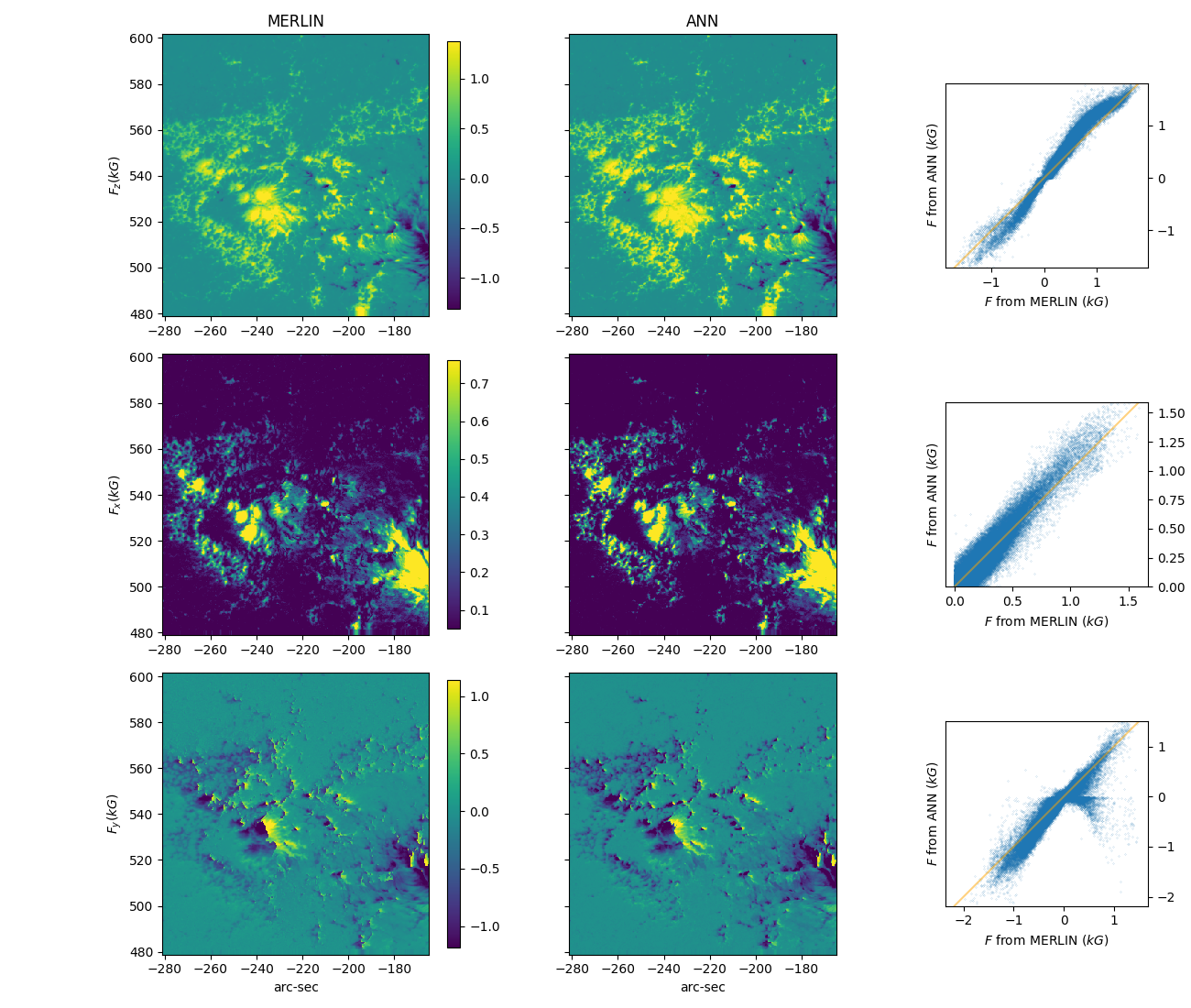
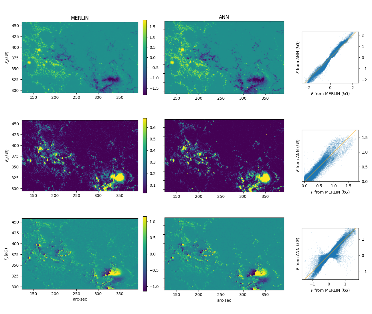
The accuracy of the ANN in recovering the magnetic field is not relevant for the purposes of this paper. Nevertheless, we show here similar comparisons for the sake of completeness. We processed two active region maps observed with Hinode/SP (more details in section 4.2 below). These maps are 384$\times$384 (map1) and 871$\times$512 (map2) spatial pixels. The ANN inversions took 4 and 11 seconds, respectively. Standard inversions with the MERLIN code are available for these maps. Figures 4 and 5 show the comparison of the magnetic flux inferred by MERLIN and our ANN. For consistency with the training set, the 180-degree ambiguity is resolved by choosing the solution that has a positive component along the $x$ axis.

3.1 Reconstruction fits

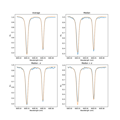
A common problem with ANN-based inversions is that they are not based on fitting the observations, unlike $\chi^{2}$ fitting methods. The quality of a fit is usually a good indicator to assess the validity of the results. Our approach suffers from this limitation too but it does provide enough information to reconstruct a model atmosphere and, from there, synthesize spectral profiles that can then be compared to the observations. It does not provide the same information as a fit because the reconstruction of the atmosphere implies additional approximations. Nevertheless, it is still useful information.

We take the parameters from the ANN inversion and compute model atmospheres by interpolating them in optical depth. For the temperature stratification, we perform a cubic interpolation of the five temperatures between $\log\tau_{500}$ $=0$ and $-4$. Above $\log\tau_{500}$$=-4$ we impose that the stratification becomes flat. In the deeper layers below $\log\tau_{500}$ $=0$, the temperature gradient usually becomes steeper. After some experimentation, we concluded that a gradient that is 30% larger than between $\log\tau_{500}$ $=0$ and $-1$ works best in reproducing the observations. Hydrostatic equilibrium is imposed and the plasma equation of state is solved numerically to determine gas and electron densities, ionization stages and relevant molecules. The magnetic field and bulk Doppler velocities are taken as constant with height from the ANN inversion.

We computed the synthetic profiles from the models reconstructed from the ANN outputs, obtaining the results shown in Fig 6. These ”reconstruction fits” support the notion that the temperature stratification retrieved by the ANN is consistent with the observations. The first panel shows the average profiles over the entire region. The other three are selected representative samples of profiles having a value of $\chi^{2}$ equal to the median over the region, and the median plus/minus a standard deviation of all $\chi^{2}$ values.

Figure 6: Upper left: Average observed and synthetic profiles in the region. Upper right: Sample profiles where the $\chi^{2}$ is equal to the median in the region. Lower left: Profiles representative of a good reconstructed fit, where the $\chi^{2}$ is equal to the median minus one standard deviation. Lower right: Profiles representative of a poor reconstructed fit, where the $\chi^{2}$ is equal to the median plus one standard deviation. In all cases, the profile in blue is the observation and orange is the synthesis from the reconstructed model atmosphere (reconstructed fit).

4 Results

We employed the ANN-based inversions described in the previous sections to explore the thermal stratification of the solar photosphere. The maps discussed above are in agreement with previous works in showing a rich thermal structure, rapidly changing with height. In this paper, we compare the spatial distribution to what is observed in the Ca II or G-Band filtergrams.

4.1 Quiet Sun

We start by considering the quiet Sun map inverted in the tests of section 3. The maps are 200$\times$200 pixels but the field of view is not exactly square because the slit stepping, which establishes the sampling in the $x$-direction, does not necessarily match the pixel size. In this case the sampling reported in the file headers is 0.15$\times$0.16 arc-seconds per pixel.

The first recognizable pattern that stands out is the similarity of the mid-photosphere temperature map to the Doppler velocity distribution. This is the well known reversed granulation effect, a natural consequence of convective motions. The tightest correlation in our dataset, shown in Figure 7, is between temperature at $\log\tau_{500}$ $=-2$ and the Doppler velocity ($v_{z}$), with a Pearson’s correlation coefficient of 0.45 (recall that, as noted above, the velocities retrieved by our procedure are at the base of the photosphere). Reversed granulation is characterized also by an anticorrelation with the $\log\tau_{500}$ $=0$ map, which in our data is of $-0.37$.

Figure 7: Scatter plot of the mid-photospheric temperatures and the Doppler velocities retrieved by the ANN.

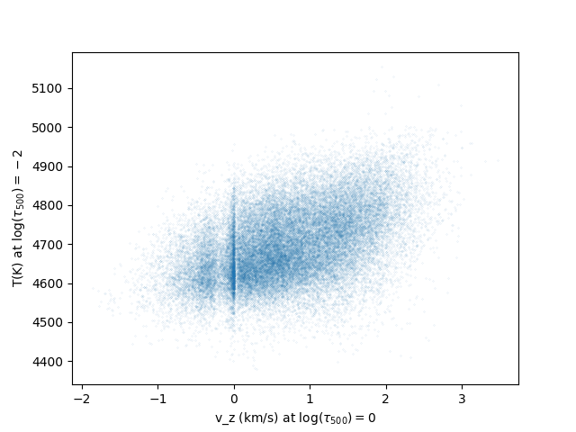
The scatter plot exhibits some vertical features. These are the result of the ANN assigning nearly the same value of $v_{z}$ to many different profiles instead of smearing them over the uncertainty range of that parameter. In least-squares inversions, the solutions for similar profiles tend to be spread over the error bar for that parameter because each inversion has followed a different path on the $\chi^{2}$ hypersurface. However, an ANN might end up assigning a specific value for a parameter (or a narrow range of values) as a ”sticky solution” for a range of input profiles. This means that the resulting maps will usually be less noisy but the noise level should not be considered an indication of the uncertainties.

Figure 8: Comparison of temperatures at different heights, as retrieved by the ANN inversion, to Ca II  filtergram (bottom right panel) in a quiet Sun region.

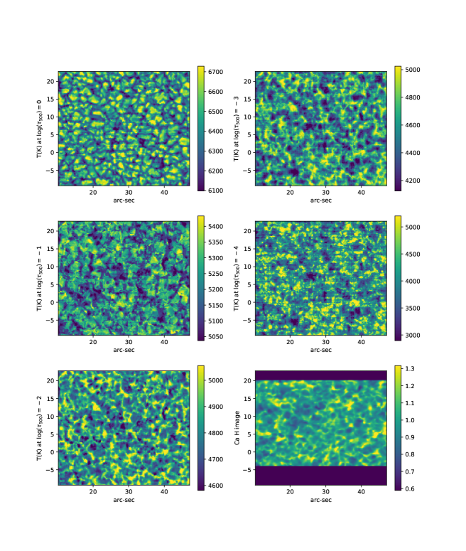
The temperature maps retrieved in the ANN inversions show a different network structure at each atmospheric height. Bright photospheric networks have been observed in the wings of the Ca II lines and in the G-Band, which are also accessible to Hinode’s narrow band instrument (Hinode/NB). It is then of interest to investigate whether these structures are related to those, both in the quiet Sun and active regions.

Figure 8 shows a comparison of the temperature maps to a simultaneous Ca II image from Hinode/NB. Alignment of SP and NB observations is not straightforward. We made use of the pointing information stored in the data headers to bring both datasets to a common reference frame. It should be noted, however, that the alignment is only accurate to a few arc-seconds .

The figure shows no obvious similarities between the Ca II  intensity and the photospheric temperatures retrieved at any of the heights. The very weak magnetic fields in this quiet region do not appear to be correlated to the Ca II  filtergram, either.

4.2 Active regions

In this section we analyze two large-field active-region maps for which there exists simultaneous G-Band and Ca II  imaging. The datasets were acquired on January 11, 2010 around 18:30 UT (map1) and January 22, 2012 around 06:30 UT (map2). The spatial sampling is coarser than in the quiet Sun observations (0.30 and 0.32 arc-seconds in the $x$ and $y$ directions, respectively) to encompass a larger field of view. Map1 consists of 384$\times$384 spatial pixels, while map2 is 871$\times$512. The full maps are shown in Figs 9 to 10, with the various panels displaying temperatures at various heights, along with the narrow-band images (the magnetic field was already introduced in Figs. 4 and 5).

Figure 9: ANN inversion of map1 (active region) at different heights (except $\log\tau_{500}$= 0) alongside G-band and Ca II  filtergrams. The arrow points in the direction to the nearest solar limb.

Figure 10: ANN inversion of map2 (active region) at different heights (except $\log\tau_{500}$= 0) alongside G-band and Ca II  filtergrams. The arrow points in the direction to the nearest solar limb.

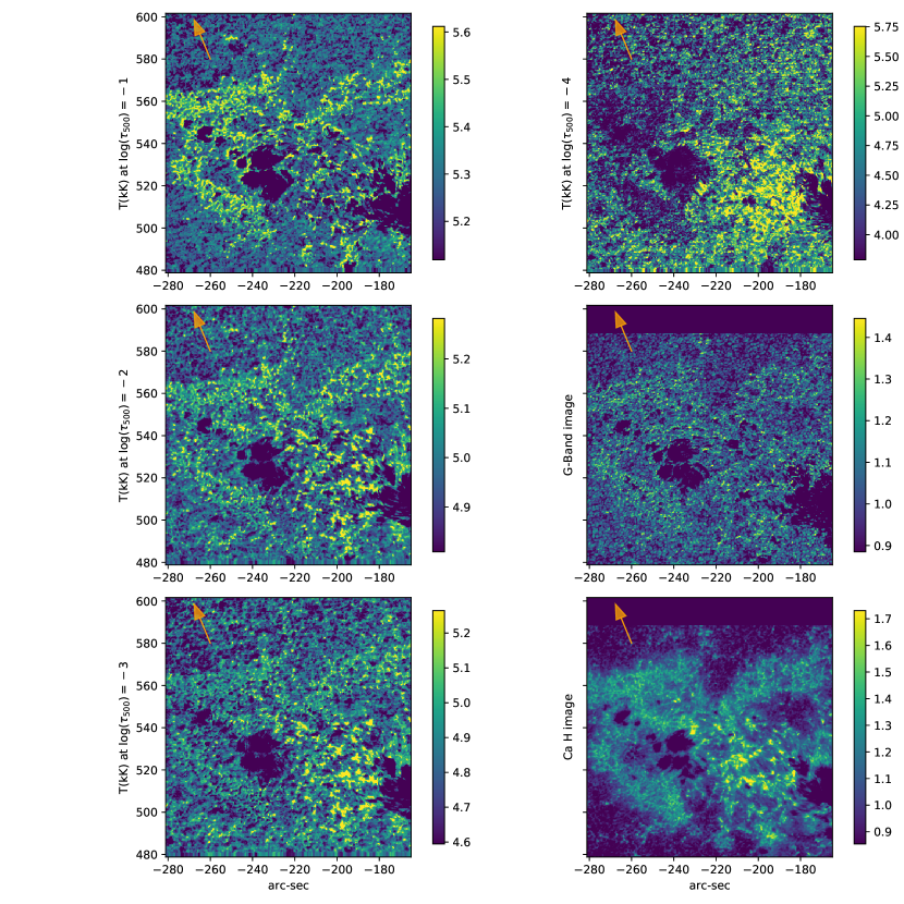
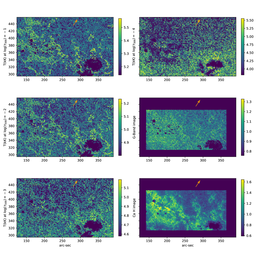
The data shows a fine network of hot pixels that roughly follows, in the mid-photosphere, the magnetic field distribution ($\log\tau_{500}$ $=-1$ and $-2$). Higher up the structure is more patchy and does not follow the magnetic field maps. Each layer exhibits a different structure and, more importantly, they also differ from both the G-Band and Ca II  H images. We discuss these differences below.

A reversal of hot and cool areas between the middle and the upper photosphere is also apparent. For instance, the lower left corner of both maps (Figs. 9 and 10) is cool at $\log\tau_{500}$ $=-1$ but hot at $\log\tau_{500}$ $=-4$ (upper left and upper right panels in both figures). The same anticorrelation is apparent in the upper left and lower right corners of map2 (Fig. 10). In fact, most of the region left of $x=200$ arc-sec in Fig. 10 has a reversed appearance. The hot network at $\log\tau_{500}$ $=-1$ (upper left panel) is seen as a dark shadow at $\log\tau_{500}$ $=-4$ (upper right panel). The same is true about the area left of $x=-240$ in map1 (Fig. 9). We quantified this by selecting only the pixels that are hot in either layer ($T>$5400 at $\log\tau_{500}$ $=-1$ or $T>$5000 at $\log\tau_{500}$ $=-4$) and computing the Pearson’s correlation coefficient. The values obtained are $-0.77$ in map1 and $-0.78$ in map2.

The temperature maps do not match the narrow-band images. There is some similarity between the temperature at $\log\tau_{500}$ $=-1$ and the G-Band image in the overall distribution of the hot network. However, a closer look shows important differences (see discussion of Fig. 11 below).

The comparison with the Ca II  H images is even more puzzling. The Ca emission follows the pattern of the hot pixels in the mid-photosphere at $\log\tau_{500}$ $=-1$ instead of the upper photosphere, as one would have expected (recall that, as discussed above, the distribution of hot pixels at $\log\tau_{500}$ $=-4$ is anticorrelated with that at $\log\tau_{500}$ $=-1$). However, the Ca images show small-scale filamentary structure in the network, as opposed to the chains of dots that appear in the temperature maps. The appearance of filaments would suggest that we are seeing higher layers but the brightness distribution follows that of the mid-photosphere. We speculate that the most plausible explanation is that the this spectral band has contributions to its response function from both the low photosphere and the (low) chromosphere. Detailed radiative transfer modeling would be necessary to confirm this point but it would require some knowledge of the chromospheric conditions, which is not available from these data.

Figure 11 shows a zoom on two regions containing several pores in both maps. The magnification is different in each figure because the area with pores is larger in map2. Even though the G-Band bright points extend over the same area as the hot network at $\log\tau_{500}$ $=-1$, they do not exhibit the same features when seen at high resolution.

Figure 11: Enlargement of of the areas with pores in the active regions map1 (upper panels) and map2 (lower panels). The left panels show ANN temperature reconstructions at $\log\tau_{500}$=-1 and the right panels, the respective G-band filtergrams. Notice the bright arcs around the limb-side (indicated by the orange arrow) of the pores in the left panels.

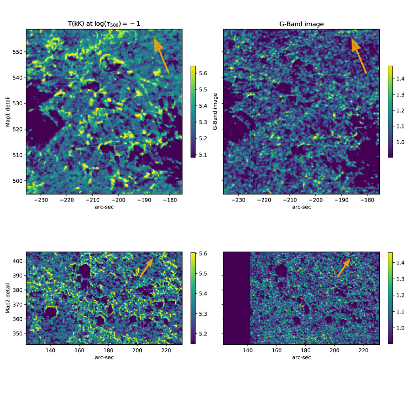
A very remarkable feature in these images is the presence of a bright arc around the edge of pores, tracing the limb side (the arrows indicate the direction to the closest limb). These arcs are visible around virtually every pore in both datasets. They have a width of one or two pixels, suggesting that they are not fully resolved in the observations, and their temperature is always between 5,600 and 5,700 K. By contrast, the pores have temperatures mostly of 4,600 to 4,800 K but in some cases, particularly the larger ones in map2, they may go down to 3,600 K, such as in the feature at coordinates (165,390) of map2.

The bright arcs are probably the pores’ ”hot walls”. The idea of a hot wall seen in perspective was introduced in early fluxtube models to explain the center-to-limb variation of faculae and G-band points (Spruit 1976; Knoelker & Schuessler 1988; Topka et al. 1997). Spruit’s original work considered unresolved fluxtubes and small pores of up to 1,000 km. The pores in our observations are significantly larger, starting from roughly 3,500 km, but there is no reason why the same effect should not take place in these.

5 Conclusions

ANN-based inversions are enabling the analysis of large spectroscopic (and spectropolarimetric) datasets. One such application is presented in this paper. The training strategy appears to be sufficiently robust for application to real observations in various situations.

It is puzzling to find such a clear anticorrelation in the location of hot points in the middle and upper photosphere. This is counterintuitive and warrants further work to confirm it, since it appears to challenge the generally accepted idea that small magnetic elements act as channels to propagate energy into the upper atmosphere (e.g., Jefferies et al. 2006; Rajaguru et al. 2019). One possibility is that the energy dissipation and associated heating might occur at higher layers than we observe here. That would explain the presence of hot points at intermediate heights that do not exhibit a temperature enhancement in the upper photosphere. However, this would not explain the patches with hot points in the upper layers that appear as quiet lower down.

In our ANN approach, each pixel is inverted independently of the rest. Therefore, the spatial distributions obtained cannot be artifacts of the procedure, they must be present in the data somehow. A possible mundane explanation for the pixels that are hot in middle layers and quiet at the top could be that the ANN is not properly trained for such situations and the closest models in the training set that reproduce the lower and mi layers are quiet in the upper layers. However, that would not explain the opposite scenario in the anticorrelation, i.e. the patches with quiet lower and middle photosphere having enhanced temperature in the upper layers.

Another important result presented in this paper is the first observation of the ”hot wall” effect, which has been a model prediction since the 1970 (Spruit 1976) and explains the bright appearance of small magnetic elements. The original theoretical models considered smaller pores of up to 1,000 km but we have detected it here in structures of at least 3,500 km. Hot walls are believed to be responsible for the brightness of faculae and small magnetic flux elements (e.g., Topka et al. 1997). This view, which is now the community consensus, is strongly reinforced by our data.

Our results open the possibility of a future application to chromospheric lines. The chromosphere is much more complicated to simulate due to NLTE radiative transfer, much faster and vigorous dynamics, faster wave phase velocities, etc. As a result, MHD numerical models are not yet sufficiently realistic that they can be used to match the observations and this limits the ability to train an ANN with chromospheric simulated profiles. However, our training strategy does not require a full numerical model. In principle one could apply a similar training using semiempirical 1D models with random perturbations to produce a large number of NLTE profiles. The computational effort involved in the database generation would be significantly higher than here but still feasible.

An area of improvement that we have found with this technique is the ”sticky solution”, where the ANN returns basically the same values within a broader uncertainty range, creating the vertical features seen in the scatter plot of Fig 7.

Finally, we would like to mention a negative result. In spite of our best efforts with this approach, we have not been able to retrieve gradients in the magnetic field or the Doppler velocity. We have encountered the same inability to retrieve gradients in previous works with other ANNs. It is not clear to us whether this inability is due to a specific problem with our methodology or an intrinsic limitation of the procedure. An interesting line for future work would be to explore these and other limitations.