Cisco at AAAI-CAD21 shared task: Predicting Emphasis in Presentation Slides using Contextualized Embeddings

Abstract

This paper describes our proposed system for the AAAI-CAD21 shared task: Predicting Emphasis in Presentation Slides. In this specific task, given the contents of a slide we are asked to predict the degree of emphasis to be laid on each word in the slide. We propose 2 approaches to this problem including a BiLSTM-ELMo approach and a transformers based approach based on RoBERTa and XLNet architectures. We achieve a score of 0.518 on the evaluation leaderboard which ranks us 3^rd and 0.543 on the post-evaluation leaderboard which ranks us 1^st at the time of writing the paper.

Introduction

Emphasis Selection for written text in visual media from crowdsourced label distributions was first proposed by Shirani et al. (2019) and then by Shirani et al. (2020a) in SemEval-2020 Task 10, Emphasis Selection for Written Text in Visual Media (Shirani et al. 2020b). AAAI-CAD21 shared task: Predicting Emphasis in Presentation Slides (Shirani et al. 2021) builds on the same SemEval-2020 Task 10. Presentation slides have become quite common in workplace scenarios and researchers have previously developed resources that guide presenters on the aspects of overall style, color, and font sizes to ensure that the graphical representation of the slide creates an impact on the viewer’s mind and the viewer can relate and understand the message that the presenter is trying to relay through the slide. This shared task aims at designing automated approaches to predict which word in the slide should be emphasized (making bold or italics) to improve the visual appeal of the slide. A pictorial example of what this shared task aims to achieve can be seen in Figure 1.

Figure 1: The left slide is plain text. The right side shows the important emphasized words in the slide.

To solve this problem we treat this task as a sequence labelling problem. Given the contents of an entire slide $d$ = {$w_{1}$, $w_{2}$, …, $w_{n}$} as the input text, we predict the emphasis probability for each word in the contents of the slide $e$ = {$e_{1}$, $e_{2}$, …, $e_{n}$}.

We mainly try two approaches to solve this problem. In our transformers approach, we experiment with two different transformer based model architectures, namely RoBERTa (Liu et al. 2019) and XLNet (Yang et al. 2019). Our choice of transformer architectures is inspired by the best performing architectures in SemEval-2020 Task 10, Emphasis selection for written text in visual media (Singhal et al. 2020; Anand et al. 2020). Both these models were pre-trained on large amounts of unannotated data in an unsupervised manner. A particular token $w$ in a slide is first passed through these transformer models to obtain embedding of each word in the form of vector representations, after which these vectors are passed through BiLSTM and fully connected layers for classification. We also keep the transformer part of the model trainable and fine-tune the weights on our downstream task of emphasis prediction.

In our second approach, we use a BiLSTM + ELMo model inspired by the baseline paper (Shirani et al. 2019). We modify the baseline model and use character embeddings together with pre-trained ELMo embeddings of each word and feed them to BiLSTM + Attention and fully connected layers for predicting emphasis scores. Additionally, we also concatenate some word-level features in the attention output before feeding it to the fully connected layers. A part of our modification is inspired by the team that stood 3rd on the SemEval-2020 Task 10 leaderboard (Singhal et al. 2020).

Additionally, we employ 2 approaches to training all models , i.e, BCE or Binary Cross Entropy Loss to directly predict emphasis probabilities and also KL Divergence Loss (Kullback and Leibler 1951) which uses Label Distribution Learning (LDL) (Geng 2016) to learn the probabilities of both emphasis and non-emphasis as used in the baseline paper (Shirani et al. 2019).

Literature Review

A lot of work in NLP has been done on keyphrase extraction in long texts from scientific articles or news (Augenstein et al. 2017; Zhang et al. 2016). Keyword detection mainly focuses on finding important nouns or noun phrases from the input text. Emphasis prediction on the other hand focuses on the automated emphasizing of words in the input text that increase the visual appeal of the text and makes it easier for the viewer of the text to understand the actual message trying to be relayed through it.

Word emphasis prediction has also been explored in spoken data using acoustic and prosodic features (Mishra, Sridhar, and Conkie 2012; Chen and Pan 2017). Emphasis Selection for written text in visual media was first proposed by Shirani et al. (2019) and then by Shirani et al. (2020a) as a SemEval-2020 Task. The baseline paper (Shirani et al. 2019) uses end-to-end label distribution learning (LDL) to predict emphasis scores on short text. The model has an embedding layer which is either Glove (Pennington, Socher, and Manning 2014) or ELMo (Peters et al., 2018) followed by BiLSTM + Attention and fully connected layers. They used Adobe Spark Dataset for their experiments. Hereon this model will be referred to as the ”Baseline” model in our paper.

Team ERNIE (Huang et al. 2020) from Semeval-2020 Task 10 who stood 1^st on the leaderboard, investigated the performance of several transformer-based models including ERNIE 2.0, XLM-RoBERTa, RoBERTa, ALBERT together with a combination of pointwise regression and pairwise ranking loss. The authors also tried some augmentation schemes and word-level lexical features and reported ERNIE 2.0 with the addition of lexical features to be the best performing model on the shared-task dataset.

Team IITK (Singhal et al. 2020) that stood 3^rd on the leaderboard also explored a number of transformer-based datasets including variations of BERT, RoBERTa, XLNet, GPT-2 and XLNet and also a modification on the baseline model. Parts of our modification on the baseline model are also based on this model reported here. Their final results were obtained from a simple ensemble of a number of their transformer-based models.

Team MIDAS (Anand et al. 2020) which stood 11^th on the leaderboard also used BERT, RoBERTa and XLNet together with a combination of either BiLSTM and Dense or just Dense layers.

Learning from annotations from different annotators has been explored with majority voting (Laws, Scheible, and Schütze 2011) or by learning individual annotator expertise (Yang et al. 2018; Rodrigues and Pereira 2017; Rodrigues, Pereira, and Ribeiro 2013). Most work on this takes only one label sequence as correct. The baseline paper (Shirani et al. 2019) was the first work to have used Label Distribution Learning (Geng 2016) for a sequence labeling task. We also explore this learning scheme in the experiments mentioned in our paper together with Binary Cross Entropy loss on probabilities obtained from the dataset annotations.

Background

Problem Definition

Given a sequence of words or tokens $d$ = {$w_{1}$, $w_{2}$, …, $w_{n}$} in a slide, the task is to compute a probabilistic score $e_{i}\>\epsilon\>[0,1]$ for each $w_{i}$ in $d$ which indicates the degree of emphasis to be laid on the word.

Evaluation Metric

The evaluation metric for our problem is defined as follows:

For a given m (1,5 and 10), we first define 2 sets, $S_{m}^{(x)}$ - set of $m$ words with top $m$ probabilities according to ground truth and $\hat{S}_{m}^{(x)}$ - set of $m$ words with top $m$ according to the model predictions. To get $S_{m}^{(x)}$, each word in the sentence has been manually annotated by 8 annotators. Based on these 2 sets, we define $Match_{m}$ as:

$$\text{Match}_{m}=\frac{\sum_{x\in D_{\text{test}}}\left|S_{m}^{(x)}\cap\hat{S}_{m}^{(x)}\right|/min(m,|x|)}{\left|D_{\text{test}}\right|}$$ (1)

where $D_{test}$ is the dataset and $x$ is the token instance. We find $Match_{m}$ for m $\in\{1,5,10\}$ and express our final score as a simple average over all 3 of them.

Dataset

Dataset Statistics for the dataset provided in the AAAI-CAD21 shared task is shown in Table 1. Each training instance is a complete slide with all the tokens present in the slide. Additionally, the sentence-wise divisions in the slides are also provided in the data. The entire training dataset was annotated by a total of 8 annotators on token-level emphasis. The dataset was annotated with a $BIO$ tagging scheme where each annotator either annotated the token as an emphasized token $(B\>or\>I)$ or not $(O)$. Thus, the probability of emphasis for each token was calculated as an average score of all annotations. The annotation scheme and the emphasis probability calculation has been shown with an example in Table 3. More information about the task and data creation can be found in Shirani et al. (2021).

	Total Slides	Total Sentences	Total Tokens
Train	1241	8849	96934
Dev	180	1175	12822
Test	355	2569	28108

Table 1: Train, Development and Test Dataset Description

	Min	Max	Average
Train	13	180	78
Dev	15	164	71
Test	17	181	79

Table 2: Token length description

Words	A1	A2	A3	A4	A5	A6	A7	A8	Freq.[B+I,O]	Probs.
•	O	O	O	O	O	O	O	O	[0,8]	0.0
Have	O	O	O	O	O	O	O	O	[0,8]	0.0
population	O	B	O	O	B	O	O	O	[2,6]	0.25
counts	O	O	O	O	O	O	O	O	[0,8]	0.0
for	O	O	O	O	O	O	O	O	[0,8]	0.0
three	O	B	O	O	O	O	O	B	[2,6]	0.25
key	O	I	O	O	O	O	O	I	[2,6]	0.25
species	O	I	B	O	B	O	O	I	[4,4]	0.5

Table 3: Annotation scheme and emphasis probability calculation on a sample sentence from the Train dataset.

System Description

Token Level Features

We tried investigating the data to find token level features that can enhance the performance of our BiLSTM-ELMo model. We tried finding features by analyzing a particular feature’s average emphasis score and the number of times a word with that feature occurred in our dataset. The average emphasis scores of the token with these features and the total count can be found in Table 4. Initially, we tried only shape and syntactic features of words by concatenating them with the attention output as described in our system description. The only feature that had given us an improvement over the baseline score was POS (Parts of Speech) tags.

Figure 2: Word Cloud of tokens having emphasis probability of $\geq 0.5$

.

Type	Train (Avg/Nos.)	Dev (Avg/Nos.)
Punctuation	0.031/14726	0.034/2082
UpperCase start	0.136/21195	0.157
Contain numbers	0.045/2893	0.055/308
All Upper Case	0.092/4498	0.116/523
Inside Brackets	0.002/3598	0.009/7560
Keyphrase Tags	0.25/12723	0.35/1179
Overall	0.102/96934	0119/12822

Table 4: Average Emphasis Scores and Count

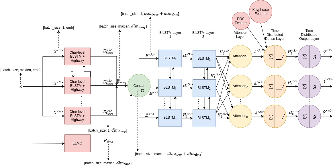
Figure 3: The BiLSTM-ELMo Model

Upon analysis of words with an emphasis score $\geq 0.5$ we noticed that most of them were scientific keywords. Thus we created our own feature by training a sequence labeling BiLSTM-CRF model with BERT (Peters et al. 2018a) word embeddings as input to the model with the information extraction datasets used for scientific keyphrase extraction by Sahrawat et al. (2019) . We use the python flair library for this task. The results of the model trained for this task are given in Table 5. The model was trained and inferred with a $BIO$ tagging scheme and it was processed to a binary feature where “B” and “I” tags were termed as 1 and “O” as 0. This feature when used together with POS tags gives us a decent improvement on the baseline results. We name this feature the “Keyphrase Feature” in all our experiments.

	Precision	Recall	f1-score	Support
B	0.6359	0.5510	0.5904	5294
I	0.6413	0.6572	0.6492	6561
O	0.9313	0.9395	0.9354	61941
Macro avg	0.7362	0.7159	0.7250	73796
Weighted avg	0.8844	0.8866	0.8852	73796

Table 5: Keyphrase Extraction Model Results

Our Approach

BiLSTM-ELMo Approach

Our BiLSTM-ELMo approach is inspired by the baseline paper (Shirani et al. 2019) where we extract the ELMo embeddings (Peters et al. 2018b) $E_{ELMo}$ for each word in a sequence and additionally, we pass the input through a character-level BiLSTM Network where the combined forward and backward embedding for the last character of each word is then passed through a Highway Layer (Singhal et al. 2020) which effectively provides us with contextual word-level embeddings $E_{hway}$ for our entire sequence. These contextual word-level embeddings are then concatenated with the extracted ELMo Embeddings for each word to produce the final word embeddings $E$.

We pass $E$ through a BiLSTM Layer followed by an Attention Layer. The output of the attention layer is then concatenated with the POS tags (Singhal et al. 2020) and Keyphrase Feature. for the corresponding word at each time-step. Now combined, the attention output and the external features are fed to a Time Distributed Dense Layer followed by our Time Distributed Output Layer. The activation function $g$ of the Output Layer is either Sigmoid or Softmax depending on whether the Loss Criterion is Binary Cross-Entropy Loss (in case of Sigmoid Activation) or Kullback-Liebler Divergence Loss (in case of Softmax Activation) used for Label Distribution Learning (LDL).

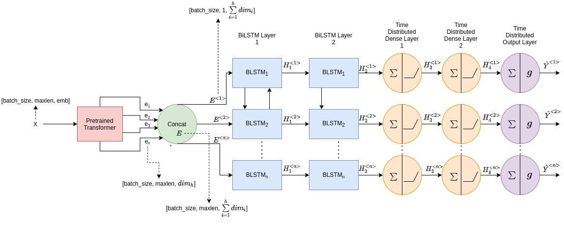
Figure 4: The Transformer-Based Model

Transformers Approach

Our Transformers approach makes use of one of two Transformer Architectures that is, XLNet or RoBERTa. First, the tokenized word input is passed through the transformer architecture and the outputs of all encoding layers of the transformer are concatenated together to get the final embedding $E$ for any given word. This embedding $E$ is now fed through a BiLSTM Layer followed by a set of Time Distributed Dense Layer. Finally, the output of the Time Distributed Dense Layers are fed to our Time Distributed Output Layer with Activation Function $g$. Here, $g$ can either be Sigmoid or Softmax when Loss Function is Binary Cross-Entropy or KL-Divergence respectively.

Experimental Setup

We use PyTorch Framework for our Deep Learning models along with the Transformer implementations, pre-trained models and, specific tokenizers in the HuggingFace library.

In the BiLSTM-ELMo Approach, we use a hidden size of 300 for the character-level LSTM Layers and on top of that, we use one highway layer which gives us word-level embeddings $E_{hway}$. These embeddings are then concatenated with their corresponding ELMo embeddings $E_{ELMo}$ where the embeddings have 2048 dimensions. This concatenated vector is passed through a BiLSTM Layer with an output size of 512 dimensions in each direction. The Attention Layer uses a self-attention mechanism, the output of the attention mechanism is concatenated with the POS tags and Keyword Feature for each word so that this information can be used by the classifier to make better predictions. The final stage of the classifier consists of a Time Distributed Dense Layer with a hidden size of 20 and ReLU Activation. Finally, the output layer has 1 output neuron if the activation function is Sigmoid and the loss function is Binary Cross-Entropy and 2 output neurons in case of a Softmax activation function and KL-Divergence Loss Function. The dropout layer probabilities were set to 0.3 for all layers to avoid overfitting.

In the transformers approach, we used the RoBERTa and XLNet transformers without freezing any layers of the network and the output of all encoder layers are concatenated to make word-level embeddings $E$. These word embeddings are then passed through two BiLSTM Layers with an output size of 256 dimensions in each direction. The output is then fed to a pair of BiLSTM Layers with 256-dimensional output in both directions. In the classifier, the output of the BiLSTM is fed to a pair of Time Distributed Dense Layers with a hidden layer size of 20 and ReLU Activation and finally to the Time Distributed Output Layer which has either 1 or 2 output neurons depending on whether the activation function used is Sigmoid or Softmax respectively. Dropout Layers with Dropout Probability 0.3 are also added to prevent overfitting.

When using Sigmoid activation, we aim to predict a single output $\hat{y}^{<t>}$ which represents the probability of emphasis to be laid on the $t^{th}$ token. This probability is used with the Binary Cross-Entropy Loss to train the model. However, in the case of Softmax, we predict a probability distribution $\hat{Y}^{<t>}$ over 2 classes $\{0=no\>emphasis,1=emphasis\}$. This distribution is used with the KL-Divergence Loss function to perform Label Distribution Learning. The equations for $\hat{y}^{<t>}$ and $\hat{Y}^{<t>}$ are as follows:

$${\hat{y}}^{<t>}=Sigmoid(z^{<t>})$$ (2)

Where $z^{<t>}$ is the logit of the last output layer for the $t^{th}$ token.

$${\hat{Y}}^{<t>}=\{Softmax(z_{0}^{<t>}),Softmax(z_{1}^{<t>})\}$$ (3)

Where $z^{<t>}_{i}$ is the logit of the last output layer for the $t^{th}$ token and $i^{th}$ class.

In both the Transformers and BiLSTM-ELMo approaches, the Binary Cross-Entropy (BCE) Loss as well as the KL-Divergence (KLD) Loss were used to train the models. The $Match_{m}$ score is used as an evaluation for all our models. The equations for both the loss functions are as follows:

$$BCE(y^{<t>},\hat{y}^{<t>})= -y^{<t>}.\log(\hat{y}^{<t>})$$

$$-(1-y^{<t>}).\log(1-\hat{y}^{<t>})$$ (4)

Where $y^{<t>}\in\{0,1\}$ is the true label for emphasis laid on each token and $\hat{y}^{<t>}$ is the output of the sigmoid activation for each token.

$$KLD(Y^{<t>}||\hat{Y}^{<t>})=\sum Y^{<t>}.\log\left(\frac{Y^{<t>}}{\hat{Y}^{<t>}}\right)$$ (5)

Where $Y^{<t>}$ is the true probability distribution for the emphasis laid on each token and $\hat{Y}^{<t>}$ is the output distribution of the softmax activation for each token.

We use the Adam Optimizer for training the models with a learning rate of 1e-4 for the BiLSTM-ELMo model for 100 epochs and 2e-5 for the Transformer-based models for 100 epochs. The training was performed on 1 NVIDIA Titan X GPU. Our code is available on Github.

Results

In Table 6 we present scores for both our BiLSTM-ELMo and Transformers approach trained on both BCE Loss and KLDivergence Loss for LDL. As we can see in the results, LDL as used by (Shirani et. al 2019) doesn’t give a huge improvement over results and at times even diminishes the results.

Model	Dev	Test
BiLSTM-ELMo (Baseline)	-	0.475
BiLSTM-ELMo (POS)	0.497	0.484
BiLSTM-ELMo (POS) (LDL)	0.501	0.506
BiLSTM-ELMo (POS, Keyphrase)	0.515	0.496
BiLSTM-ELMo (POS, Keyphrase)	0.504	0.501
(LDL)
XLNet	0.536	0.514
XLNet (LDL)	0.529	0.491
RoBERTa	0.51	0.485
RoBERTa (LDL)	0.515	0.47

Table 6: Performance of BiLSTM-ELMo and Transformers approach on development and Test set. The results are expressed in terms of average $Match_{m}$ for m $\in\{1,5,10\}$. LDL indicates that label distribution learning was employed to train the model with KL-Divergence as the loss function, Binary Cross Entropy otherwise. For BiLSTM-ELMo model the extra features concatenated at the attention layer have been mentioned with each experiment. Baseline. indicates the scores by the baseline model defined by Shirani et al. (2019)

For our final submissions, we tried an ensemble of scores from different models shown in Table 7. Our best scores on the Evaluation leaderboard were obtained using an ensemble of XLNet and RoBERTa with LDL where we stood 3rd. Meanwhile, our best scores on the Post-Evaluation leaderboard were obtained using an ensemble of XLNet and BiLSTM-ELMo approach with POS tags and Keyphrase Feature where we currently stand 1st on the leaderboard.

Model	Dev	Test
XLNet + RoBERTa (LDL)	0.547	0.518
XLNet + BiLSTM-ELMo (Keyphrase)	0.538	0.532
XLNet + BiLSTM-ELMo (LDL)	0.55	0.543

Table 7: Performance of different ensemble models

Additionally, we also ran experiments by dividing the presentations into their constituent sentences in the train and development data. Thus each training instance now corresponds to a particular sentence belonging to a presentation slide in the original corpus. The development set results can be found in Table 8. The evaluation scheme used in this experiment uses the same Match_m as described in the Evaluation Metric section but with m = $1,2,3,4$ as used in Shirani et al. (2020a).

Model	Dev
XLNet	0.758
XLNet (LDL)	0.757
RoBERTa	0.743
RoBERTa (LDL)	0.745
BiLSTM-ELMo	0.751
BiLSTM-ELMo (LDL)	0.752

Table 8: Sentence-wise results on the Development set

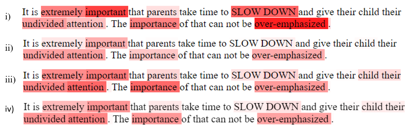
Figure 5: Emphasis Heatmaps i) Ground Truth ii) BiLSTM-ELMo iii) XLNet iv) Best Ensemble Model

Analysis

Length vs Performance

We wanted to understand how the performance of our models was affected by the length of the instances. Table 9 summarizes the performance of our best performing single model, i.e, XLNet on the development set divided into three sets, Short ($\leq 40$ tokens, 80 samples), Medium (40 to 90 tokens, 262 samples), and Long ($>$90 tokens, 50 samples). As we can see, the model performance deteriorates with the increasing length of the instances.

	XLNet
Small ($\leq 40$)	0.648
Medium ($>$40 and $\leq 90$)	0.549
Large ($>$90)	0.42

Table 9: Average $Match_{m}$ for best performing XLNet model on different size of instances in the development set

Emphasis vs Parts of Speech

Table 10 shows POS (Parts of Speech) tags vs. average emphasis on the development dataset. We did this experiment to understand how our model predictions performed on each POS tag when compared to the actual human-annotated emphasis scores on the development set. We noticed that the original average emphasis scores were highest on Adjectives followed by Noun. On comparing our models, we found that XLNet was able to almost accurately predict the emphasis scores on Adjectives and Noun respectively, and BiLSTM-ELMo also had the highest predictions on Adjectives and Noun respectively. We also noticed that XLNet did a better job on predicting the emphasis score on different POS tags where the predictions were either very close to the human scores or marginally lesser. On the other hand, we noticed that BiLSTM-ELMo’s predictions fell short by bigger margins when compared to XLNet and gave more emphasis to Adverbs than that in the development set.

POS	Count	Human	BiLSTM	XLNet
Noun	4719	0.169	0.134	0.168
Verb	1420	0.118	0.083	0.113
Adjectives	982	0.186	0.140	0.181
Det	634	0.062	0.029	0.042
Adverbs	347	0.111	0.068	0.103
Pronouns	165	0.040	0.068	0.022
Punct	2082	0.034	0.015	0.025

Table 10: POS tags vs. average emphasis on development dataset

Conclusion

In this paper, we present our approach to AAAI-CAD21 shared task: Predicting Emphasis in Presentation Slides. Our best submission gave us an average $Match_{m}$ of 0.518 placing us 3^rd on the Evaluation phase leaderboard and an average $Match_{m}$ of 0.543 placing us 1^st on the Post-Evaluation leaderboard at the time of writing the paper. Future work includes using a hierarchical approach to emphasis prediction as a sequence labeling task using both sentence-level (individual sentence in a slide) and slide-level representations of a word (Luo, Xiao, and Zhao 2019).

References

- Anand et al. (2020) Anand, S.; Gupta, P.; Yadav, H.; Mahata, D.; Gosangi, R.; Zhang, H.; and Shah, R. R. 2020. MIDAS at SemEval-2020 Task 10: Emphasis Selection using Label Distribution Learning and Contextual Embeddings. arXiv preprint arXiv:2009.02619 .
- Augenstein et al. (2017) Augenstein, I.; Das, M.; Riedel, S.; Vikraman, L.; and McCallum, A. 2017. Semeval 2017 task 10: Scienceie-extracting keyphrases and relations from scientific publications. arXiv preprint arXiv:1704.02853 .
- Chen and Pan (2017) Chen, Y.; and Pan, R. 2017. Automatic emphatic information extraction from aligned acoustic data and its application on sentence compression. In Thirty-First AAAI Conference on Artificial Intelligence.
- Geng (2016) Geng, X. 2016. Label distribution learning. IEEE Transactions on Knowledge and Data Engineering 28(7): 1734–1748.
- Huang et al. (2020) Huang, Z.; Feng, S.; Su, W.; Chen, X.; Wang, S.; Liu, J.; Ouyang, X.; and Sun, Y. 2020. ERNIE at SemEval-2020 Task 10: Learning Word Emphasis Selection by Pre-trained Language Model. arXiv preprint arXiv:2009.03706 .
- Kullback and Leibler (1951) Kullback, S.; and Leibler, R. A. 1951. On information and sufficiency. The annals of mathematical statistics 22(1): 79–86.
- Laws, Scheible, and Schütze (2011) Laws, F.; Scheible, C.; and Schütze, H. 2011. Active learning with amazon mechanical turk. In Proceedings of the 2011 Conference on Empirical Methods in Natural Language Processing, 1546–1556.
- Liu et al. (2019) Liu, Y.; Ott, M.; Goyal, N.; Du, J.; Joshi, M.; Chen, D.; Levy, O.; Lewis, M.; Zettlemoyer, L.; and Stoyanov, V. 2019. Roberta: A robustly optimized bert pretraining approach. arXiv preprint arXiv:1907.11692 .
- Luo, Xiao, and Zhao (2019) Luo, Y.; Xiao, F.; and Zhao, H. 2019. Hierarchical Contextualized Representation for Named Entity Recognition.
- Mishra, Sridhar, and Conkie (2012) Mishra, T.; Sridhar, V. R.; and Conkie, A. 2012. Word prominence detection using robust yet simple prosodic features. In Thirteenth Annual Conference of the International Speech Communication Association.
- Pennington, Socher, and Manning (2014) Pennington, J.; Socher, R.; and Manning, C. D. 2014. Glove: Global vectors for word representation. In Proceedings of the 2014 conference on empirical methods in natural language processing (EMNLP), 1532–1543.
- Peters et al. (2018a) Peters, M. E.; Neumann, M.; Iyyer, M.; Gardner, M.; Clark, C.; Lee, K.; and Zettlemoyer, L. 2018a. Deep contextualized word representations. CoRR abs/1802.05365. URL http://arxiv.org/abs/1802.05365.
- Peters et al. (2018b) Peters, M. E.; Neumann, M.; Iyyer, M.; Gardner, M.; Clark, C.; Lee, K.; and Zettlemoyer, L. 2018b. Deep contextualized word representations. arXiv preprint arXiv:1802.05365 .
- Rodrigues and Pereira (2017) Rodrigues, F.; and Pereira, F. 2017. Deep learning from crowds.
- Rodrigues, Pereira, and Ribeiro (2013) Rodrigues, F.; Pereira, F. C.; and Ribeiro, B. 2013. Sequence labeling with multiple annotators. Machine Learning 95: 165–181.
- Sahrawat et al. (2019) Sahrawat, D.; Mahata, D.; Kulkarni, M.; Zhang, H.; Gosangi, R.; Stent, A.; Sharma, A.; Kumar, Y.; Shah, R. R.; and Zimmermann, R. 2019. Keyphrase Extraction from Scholarly Articles as Sequence Labeling using Contextualized Embeddings. arXiv preprint arXiv:1910.08840 .
- Shirani et al. (2019) Shirani, A.; Dernoncourt, F.; Asente, P.; Lipka, N.; Kim, S.; Echevarria, J.; and Solorio, T. 2019. Learning emphasis selection for written text in visual media from crowd-sourced label distributions. In Proceedings of the 57th Annual Meeting of the Association for Computational Linguistics, 1167–1172.
- Shirani et al. (2020a) Shirani, A.; Dernoncourt, F.; Echevarria, J.; Asente, P.; Lipka, N.; and Solorio, T. 2020a. Let Me Choose: From Verbal Context to Font Selection. arXiv preprint arXiv:2005.01151 .
- Shirani et al. (2020b) Shirani, A.; Dernoncourt, F.; Lipka, N.; Asente, P.; Echevarria, J.; and Solorio, T. 2020b. SemEval-2020 Task 10: Emphasis Selection for Written Text in Visual Media. In Proceedings of the Fourteenth Workshop on Semantic Evaluation, 1360–1370. Barcelona (online): International Committee for Computational Linguistics. URL https://www.aclweb.org/anthology/2020.semeval-1.184.
- Shirani et al. (2021) Shirani, A.; Tran, G.; Trinh, H.; Dernoncourt, F.; Lipka, N.; Asente, P.; Echevarria, J.; and Solorio, T. 2021. Learning to Emphasize: Dataset and Shared Task Models for Selecting Emphasis in Presentation Slides. In Proceedings of CAD21 workshop at the Thirty-fifth AAAI Conference on Artificial Intelligence (AAAI-21).
- Singhal et al. (2020) Singhal, V.; Dhull, S.; Agarwal, R.; and Modi, A. 2020. IITK at SemEval-2020 Task 10: Transformers for Emphasis Selection. arXiv preprint arXiv:2007.10820 .
- Yang et al. (2018) Yang, J.; Drake, T.; Damianou, A.; and Maarek, Y. 2018. Leveraging Crowdsourcing Data for Deep Active Learning An Application: Learning Intents in Alexa. In Proceedings of the 2018 World Wide Web Conference, WWW ’18, 23–32. Republic and Canton of Geneva, CHE: International World Wide Web Conferences Steering Committee. ISBN 9781450356398. doi:10.1145/3178876.3186033. URL https://doi.org/10.1145/3178876.3186033.
- Yang et al. (2019) Yang, Z.; Dai, Z.; Yang, Y.; Carbonell, J.; Salakhutdinov, R. R.; and Le, Q. V. 2019. Xlnet: Generalized autoregressive pretraining for language understanding. In Advances in neural information processing systems, 5753–5763.
- Zhang et al. (2016) Zhang, Q.; Wang, Y.; Gong, Y.; and Huang, X.-J. 2016. Keyphrase extraction using deep recurrent neural networks on twitter. In Proceedings of the 2016 conference on empirical methods in natural language processing, 836–845.