Overcoming finite-size effects in electronic structure simulations at extreme conditions

Abstract

Ab initio quantum Monte Carlo (QMC) methods in principle allow for the calculation of exact properties of correlated many-electron systems, but are in general limited to the simulation of a finite number of electrons $N$ in periodic boundary conditions. Therefore, an accurate theory of finite-size effects is indispensable to bridge the gap to realistic applications in the thermodynamic limit. In this work, we revisit the uniform electron gas (UEG) at finite temperature as it is relevant to contemporary research e.g. in the field of warm dense matter. In particular, we present a new scheme to eliminate finite-size effects both in the static structure factor $S(q)$ and in the interaction energy $v$, which is based on the density response formalism. We demonstrate that this method often allows to obtain $v$ in the TDL within a relative accuracy of $\sim 0.2\%$ from as few as $N=4$ electrons without any empirical choices or knowledge of results for other values of $N$. Finally, we evaluate the applicability of our method upon increasing the density parameter $r_{s}$ and decreasing the temperature $T$.

I Introduction

The accurate numerical simulation of interacting many-electron systems constitutes a central challenge in many domains of theoretical physics, quantum chemistry, material science, and related disciplines Giuliani and Vignale (2008). Yet, while the equations governing these systems have been known for approximately a century, there still does not exist a practical tool to solve them in many situations and one has to rely on approximations.

A particularly important method for this purpose is density functional theory (DFT), which has emerged as the de-facto work horse of quantum chemistry and boasts a remarkable success regarding the description of both bulk materials and molecules Burke (2012); Jones (2015). More specifically, DFT simulations are computationally efficient, as the the complicated $N$-body problem of interest is mapped on an effective single-body problem that can actually be solved numerically. Yet, this mapping comes at the expense of self-sufficiency, as information about electronic correlations must be supplied externally in the form of the in general unknown exchange–correlation functional.

In contrast, computationally more expensive quantum Monte Carlo (QMC) methods are, at least in principle, capable to provide an exact solution to the $N$-electron problem Booth et al. (2013); Anderson (2007) without any a-priory information or empirical input. In particular, it was only the seminal QMC study of the uniform electron gas (UEG) by Ceperley and Alder Ceperley and Alder (1980) which allowed for the subsequent construction of accurate electron exchange–correlation functionals Perdew and Wang (1992); Perdew and Zunger (1981); Vosko et al. (1980); Perdew et al. (1996) that made the success of DFT possible in the first place. At the same time, most QMC methods are by definition only applicable for a finite number of electrons $N$, while most physical systems are given in the thermodynamic limit (TDL), i.e., in the limit of $N\to\infty$ with the density $n=N/V$ remaining constant. This problem is substantially exacerbated by the notorious fermion sign problem Loh et al. (1990); Troyer and Wiese (2005); Dornheim (2019), which leads to an exponential increase of computation time with $N$, see Ref. Dornheim (2019) for a topical review article. In fact, the sign problem has been revealed as $NP$-hard for a certain type of Hamiltonian by Troyer and Wiese Troyer and Wiese (2005), and a general solution appears to be improbable.

For these reasons, the solid understanding of finite-size effects in QMC data and their subsequent estimation in the form of a finite-size correction (FSC) is of paramount importance for the QMC community and beyond, and constitutes a highly active topic of research Fraser et al. (1996); Kent et al. (1999); Williamson et al. (1997); Lin et al. (2001); Chiesa et al. (2006, 2007); Azadi and Foulkes (2019); Mihm et al. (2019); Holzmann et al. (2016, 2011a); Drummond et al. (2008); Holzmann et al. (2011b); Dornheim et al. (2016a, 2018a); Moroni et al. (1995); Kwee et al. (2008); Buraczynski et al. (2018); Spink et al. (2013); Brown et al. (2013); Groth et al. (2017a). Moreover, while most works have been devoted to the study of electrons at ambient conditions, i.e., in the ground state Foulkes et al. (2001), there has recently emerged a growing interest in the properties of matter at extreme densities and temperatures. Of particular importance is the regime of so-called warm dense matter Bonitz et al. (2020); Graziani et al. (2014); Dornheim et al. (2018a), which is characterized by the simultaneous importance of thermal excitations, Coulomb correlations, and fermionic exchange-effects and naturally occurs e.g. in astrophysical objects such as giant planet interiors Militzer et al. (2008) and brown dwarfs Saumon et al. (1992); Becker et al. (2014). In addition, warm dense matter has been predicted to occur on the pathway towards inertial confinement fusion Hu et al. (2011), and is routinely realized experimentally in large research centres around the globe Falk (2018).

This interest has sparked a series of new developments in the field of electronic QMC simulations at finite temperature Driver and Militzer (2012); Blunt et al. (2014); Dornheim et al. (2017a); Brown et al. (2013); Dornheim et al. (2015a); Schoof et al. (2015); Malone et al. (2015); Militzer and Driver (2015); Malone et al. (2016); Dornheim et al. (2016a, 2017b); Groth et al. (2017a); Dornheim et al. (2017c); Driver et al. (2018); Dornheim et al. (2020a, b); Lee et al. (2020); Liu et al. (2018); Yilmaz et al. (2020), which, in turn, has caused the need to understand the impact of thermal excitations on finite-size effects. In general, this problem can be re-stated as the search for a short-range property that can be accurately inferred from a QMC simulation of a finite-system and, in combination with a readily available theory such as the random phase approximation (RPA) [see Eq. (1) below], yields the full description of a system in the TDL.

In the ground state, Chiesa et al. Chiesa et al. (2006) have proposed to use the static structure factor (SSF) $S(q)$ for this purpose, which indeed has been shown empirically to only weakly depend on $N$ both at zero and finite temperature Dornheim et al. (2016a, 2018a). This finding has allowed to introduce a simple analytical first-order correction to the finite-size error of the interaction energy per particle $v$, which was subsequently generalized by Brown et al. Brown et al. (2013) to arbitrary temperatures. Yet, this correction breaks down both for high temperature and density and, thus, is inapplicable over substantial parts of the warm-dense matter regime. The full estimation of the main contribution to the finite-size error of $v$ then requires the estimation of a discretization error [see Eq. (II.4) below] using a suitable trial function, like the SSF within RPA or a more sophisticated dielectric theory like the approximate scheme by Singwi et al. Singwi et al. (1968); Tanaka and Ichimaru (1986); Sjostrom and Dufty (2013) (STLS). This was demonstrated by Dornheim, Groth, and co-workers Dornheim et al. (2016a, 2017a, 2018a), who showed that this procedure reduces the finite-size error in the QMC data by approximately two order of magnitude, allowing for a reliable subsequent extrapolation to the TDL Dornheim et al. (2016a); Groth et al. (2017b).

In the present work, we go one step further and address the source of the residual finite-size errors after the discretization error has been eliminated. To this end, we employ the density response formalism, and propose that in many cases, the static local field correction constitutes a more suitable choice for a short-range exchange–correlation function that can be accurately estimated from a QMC simulation of as few as $N=4$ particles. More specifically, our new scheme allows for a direct estimation of the finite-size error in $S(q)$ itself, which already constitutes an important finding in itself. Moreover, this FSC for the SSF can subsequently be used to eliminate the residual finite-size error in $v$, and we find that often $N=4$ particles are sufficient to estimate $v$ with a relative accuracy of $\sim 0.2\%$ without any empirical input, extrapolation, or knowledge about QMC results for multiple $N$.

The paper is organized as follows: In Sec. II, we introduce the required theoretical background, starting with the density response formalism (II.1) and the fluctuation–dissipation theorem (II.2), followed by our new theory of finite-size effects in the SSF (II.3), and the implications for the FSC of the interaction energy $v$ (II.4). The application of our scheme is demonstrated in Sec. III, starting with an extensive analysis at extreme density and temperature in Sec. III.1. In addition, we analyze the applicability of the method for the important cases of increasing coupling strength (III.2) and low temperature (III.3). The paper is concluded by a brief summary and outlook in Sec. IV.2.

II Theory

Throughout this work, we restrict ourselves to an unpolarized uniform electron gas (UEG), see Ref. Dornheim et al. (2018a) for details. In addition, the UEG is characterized by two parameters: i) the density parameter $r_{s}=\overline{r}/a_{\textnormal{B}}$, where $\overline{r}$ and $a_{\textnormal{B}}$ denote the average particle distance and first Bohr radius, and ii) the degeneracy temperature $\theta=k_{\textnormal{B}}T/E_{\textnormal{F}}$, where $E_{\textnormal{F}}$ is the usual Fermi energy Ott et al. (2018); Giuliani and Vignale (2008).

All formulas and results are given in Hartree atomic units.

II.1 Density response and local field correction

The density response of an electron gas to an external harmonic perturbation Dornheim et al. (2020a) of wave-number $q$ and frequency $\omega$ is—within linear response theory—fully described by the dynamic density response function Giuliani and Vignale (2008); Kugler (1975)

$$\chi(q,\omega)=\frac{\chi_{0}(q,\omega)}{1-\frac{4\pi}{q^{2}}\left[1-G(q,\omega)\right]\chi_{0}(q,\omega)}\ .$$ (1)

Here $\chi_{0}(q,\omega)$ denotes the density response function of the ideal Fermi gas and the information about exchange–correlation effects is contained in the dynamic local field correction $G(q,\omega)$.

Let us next consider the static limit, i.e.,

$$\chi(q)=\lim_{\omega\to 0}\chi(q,\omega)\ .$$ (2)

In this limit, accurate data for Eq. (1) have been presented by Dornheim et al. Dornheim et al. (2019a, 2020c, 2020d) based on the relation Bowen et al. (1994)

$$\chi({q})=-n\int_{0}^{\beta}\textnormal{d}\tau\ F({q},\tau)\quad,$$ (3)

with the imaginary-time density–density correlation function being defined as

$$F(q,\tau)=\frac{1}{N}\braket{\rho(q,\tau)\rho(-q,0)}\ .$$ (4)

In addition, it is possible to obtain $\chi(q)$ from a simulation of the harmonically perturbed electron gas, which has been done both in the ground state Moroni et al. (1992, 1995); Bowen et al. (1994) and at finite temperature Dornheim et al. (2017c); Groth et al. (2017a); Dornheim et al. (2020a). In principle, it is then straightforward to use $\chi(q)$ to solve Eq. (1) for the static LFC

$$G(q) = \lim_{\omega\to 0}G(q,\omega)$$ (5)

$$= 1-\frac{q^{2}}{4\pi}\left(\frac{1}{\chi_{0}(q)}-\frac{1}{\chi(q)}\right)\ .$$

For the present paper, it is important to explicitly indicate the dependence of different estimated properties on the system size, for which purpose we shall henceforth use the superscript $N$. In particular, the most simple way to write Eq. (5) is then given by

$$G^{N}(q)=1-\frac{q^{2}}{4\pi}\left(\frac{1}{\chi^{\textnormal{TDL}}_{0}(q)}-\frac{1}{\chi^{N}(q)}\right)\ .$$ (6)

Yet, we empirically know that $\chi^{N}(q)$ substantially depends on $N$, and this finite-size error is propagated into $G^{N}(q)$ as defined in Eq. (6). Fortunately, we also know that this error is almost exclusively due to the inconsistency between $\chi^{\textnormal{TDL}}_{0}(q)$ and $\chi^{N}(q)$, as the consistent determination of $G(q)$ would require us to instead use the density response function of the ideal system at the same system size, $\chi_{0}^{N}(q)$. Thus, the finite-size corrected static local field correction can be computed as Moroni et al. (1992, 1995)

$$G^{N}_{\textnormal{FSC}}(q) = 1-\frac{q^{2}}{4\pi}\left(\frac{1}{\chi^{N}_{0}(q)}-\frac{1}{\chi^{N}(q)}\right)$$

$$\approx G^{\textnormal{TDL}}(q)\ .$$

Moreover, we can readily define a FSC for $G(q)$,

$$\Delta G^{N}(q)=\frac{q^{2}}{4\pi}\left(\frac{1}{\chi_{0}^{\textnormal{TDL}}(q)}-\frac{1}{\chi_{0}^{N}(q)}\right)\ ,$$ (8)

such that

$$G^{N}_{\textnormal{FSC}}(q)=G^{N}(q)+\Delta G^{N}(q)\ .$$ (9)

II.2 Fluctuation–dissipation theorem

The fluctuation–dissipation theorem Giuliani and Vignale (2008)

$$S({q},\omega)=-\frac{\textnormal{Im}\chi({q},\omega)}{\pi n(1-e^{-\beta\omega})}$$ (10)

relates Eq. (1) to the dynamic structure factor $S(q,\omega)$ and, thus, directly connects the LFC to different material properties. In particular, the static structure factor is defined as the normalization of the DSF

$$S(q)=\int_{-\infty}^{\infty}\textnormal{d}\omega\ S(q,\omega)\ ,$$ (11)

and thus entails an averaging over the full frequency range. We stress that this is in contrast to the static density response function $\chi(q)$ introduced in the previous section, which is defined as the limit of $\omega\to 0$. The SSF, in turn, gives direct access to the interaction energy of the system, and for a uniform system it holds Dornheim et al. (2018a)

$$v=\frac{1}{\pi}\int_{0}^{\infty}\textnormal{d}q\ \left[S(q)-1\right]\ .$$ (12)

Finally, we mention the adiabatic connection formula Dornheim et al. (2018a); Groth et al. (2017b); Karasiev et al. (2014)

$$f_{xc}(r_{s},\theta)=\frac{1}{r_{s}^{2}}\int_{0}^{r_{s}}\textnormal{d}\overline{r}_{s}\ v(\overline{r}_{s},\theta)\overline{r}_{s}\ ,$$ (13)

which implies that the free energy $f$ (and, equivalently the partition function $Z$) can be inferred from either $\chi(q,\omega)$, $S(q,\omega)$, or $S(q)$.

II.3 Finite-size correction of $S(q)$

Since the full frequency-dependence of $G(q,\omega)$ remains unknown in most cases, one might neglect dynamic effects and simply substitute $G(q)$ in Eq. (1). This leads to the dynamic density response function within the static approximation Dornheim et al. (2018b); Hamann et al. (2020); Dornheim and Vorberger (2020); Groth et al. (2019),

$$\chi_{\textnormal{stat}}(q,\omega)=\frac{\chi_{0}(q,\omega)}{1-\frac{4\pi}{q^{2}}\left[1-G(q)\right]\chi_{0}(q,\omega)}\ ,$$ (14)

which entails the frequency-dependence on an RPA level, but exchange-correlation effects are incorporated statically. Indeed, it has been shown that Eq. (14) allows for an accurate (though not exact) description of many material properties Dornheim et al. (2018b); Groth et al. (2019); Dornheim et al. (2020e); Hamann et al. (2020). This finding constitutes the motivation for the present scheme to overcome finite-size effects in $S(q)$ and related quantities.

Very recently, Dornheim and Moldabekov Dornheim and Moldabekov (2021) have introduced the concept of an effectively frequency-averaged LFC $\overline{G}(q)$, i.e., a static LFC that is not defined in the limit of $\omega\to 0$, but effectively incorporates the dependence on $\omega$. For example, we can define such a LFC in a way that, when it is being inserted into Eqs. (14), (10) and (11), exactly reproduces the QMC data for $S^{N}(q)$,

$$\overline{G}^{N}_{\textnormal{invert}}(q)=\textnormal{min}_{\overline{G}}\left(\left|S_{\overline{G}}(q)-S^{N}(q)\right|\right)\ .$$ (15)

In practice, we determine $\overline{G}^{N}_{\textnormal{invert}}(q)$ numerically by scanning the corresponding results for $S(q)$ over a dense grid of $\overline{G}$ for each particular wave number $q$. In fact, it has been shown Dornheim et al. (2020e) that $G^{N}(q)$ is almost exactly equal to $\overline{G}^{N}_{\textnormal{invert}}(q)$ for wave numbers $q\lesssim 3q_{\textnormal{F}}$. It is therefore reasonable to approximate the (a-priori unknown) FSC for $\overline{G}^{N}_{\textnormal{invert}}(q)$ by the FSC for the static limit $\Delta G^{N}(q)$ defined in Eq. (9) above,

$$\overline{G}^{\textnormal{TDL}}_{\textnormal{invert}}(q)\approx\overline{G}^{\textnormal{FSC}}_{\textnormal{invert}}(q)=\overline{G}^{N}_{\textnormal{invert}}(q)+\Delta G^{N}(q)\ .$$ (16)

The resulting corrected value $\overline{G}^{\textnormal{FSC}}_{\textnormal{invert}}(q)$ is then used to compute the finite-size corrected value of the static structure factor $S_{N}^{\textnormal{FSC}}(q)$, again via Eqs. (14), (10) and (11). The corresponding value of the FSC for $S^{N}(q)$ is then given by

$$\Delta S^{N}(q)=S_{N}^{\textnormal{FSC}}(q)-S^{N}(q)\ .$$ (17)

We stress that our approach is inherently superior to the static approximation introduced in Refs. Dornheim et al. (2020e, 2018b); Hamann et al. (2020), as we only use it to estimate the finite-size error in $\overline{G}_{\textnormal{invert}}^{N}(q)$, which is comparably small. Thus, the full frequency-dependence of $G(q,\omega)$ is consistently incorporated into the definition of $\overline{G}_{\textnormal{invert}}^{N}(q)$, whereas we only neglect it for the FSC in Eq. (16).

II.4 Finite-size correction of the interaction energy

The interaction energy in the TDL is defined by evaluating the integral in Eq. (12) above using the SSF in the TDL, $S^{\textnormal{TDL}}(q)$,

$$v=\frac{1}{\pi}\int_{0}^{\infty}\textnormal{d}q\ \left[S^{\textnormal{TDL}}(q)-1\right]\ .$$ (18)

In contrast, the corresponding energy per particle for a finite system is defined as a sum over the reciprocal vectors $\mathbf{G}$ of the simulation cell,

$$\frac{V^{N}}{N}=\frac{1}{2V}\sum_{\mathbf{G}\neq\mathbf{0}}\left[S^{N}(\mathbf{G})-1\right]\frac{4\pi}{G^{2}}+\frac{\xi_{\textnormal{M}}}{2}\ ,$$ (19)

where $\xi_{\textnormal{M}}$ is the usual Madelung constant taking into account the interaction of a charge with its own background and periodic array of images Fraser et al. (1996).

Following a short analysis that has been presented elsewhere Drummond et al. (2008); Chiesa et al. (2006); Dornheim et al. (2016a, 2018a), it can be seen that there are two potential sources for the difference between Eqs. (18) and (19): (i) the discretization error $\Delta v^{N}_{\textnormal{d}}$ due to the approximation of a continuous integral by a discrete sum; (ii) the error intrinsic in $S^{N}(q)\neq S^{\textnormal{TDL}}(q)$, leading to $\Delta v^{N}_{\textnormal{i}}$.

It is well known that (i) is the dominant effect (at least for a sufficiently large system-size $N$), and it can be accurately estimated using a decent trial function for $S(q)$, e.g. using STLS Tanaka and Ichimaru (1986); Sjostrom and Dufty (2013); Dornheim et al. (2016a), or even RPA,

$$\Delta v_{\textnormal{d}}^{N}\left[S_{\textnormal{trial}}(q)\right] = \frac{1}{\pi}\int_{0}^{\infty}\textnormal{d}q\ \left[S_{\textnormal{trial}}(q)-1\right]$$

$$-\left(\frac{1}{2V}\sum_{\mathbf{G}\neq\mathbf{0}}\left[S_{\textnormal{trial}}(\mathbf{G})-1\right]\frac{4\pi}{G^{2}}+\frac{\xi_{\textnormal{M}}}{2}\right)\ .$$

In addition, we mention that the first-order contribution to Eq. (II.4) is a direct consequence of the missing $\mathbf{G}=\mathbf{0}$ term in Eq. (19), and can be exactly evaluated in RPA, which gives Chiesa et al. (2006); Brown et al. (2013); Dornheim et al. (2018a)

$$\Delta v^{N}_{\textnormal{d,0}}=\frac{\omega_{p}}{4N}\textnormal{coth}\left(\frac{\beta\omega_{p}}{2}\right)\ ,$$ (21)

where $\omega_{p}=\sqrt{r_{s}^{3}/3}$ denotes the usual plasma frequency.

Yet, often (ii), too, is not negligible, which is particularly true at either high temperature/small $r_{s}$ or in the low-temperature regime where $S^{N}(q)$ is afflicted with momentum shell effects Spink et al. (2013). Moreover, the fermion sign problem Dornheim (2019); Troyer and Wiese (2005) still prevents QMC simulations except for very small $N$ for substantial parts of the WDM regime, which makes the accurate estimation of the intrinsic error highly desirable.

We thus make use of the new FSC for $S(q)$ given in Eq. (17) above, and write the intrinsic finite-size error of $v$ as

$$\Delta v_{\textnormal{i}}^{N}=\frac{1}{2V}\sum_{\mathbf{G}\neq\mathbf{0}}\left[S_{N}^{\textnormal{FSC}}(\mathbf{G})-S^{N}(\mathbf{G})\right]\frac{4\pi}{G^{2}}\ .$$ (22)

The fully finite-size corrected estimate for the interaction energy is then given by

$$v^{\textnormal{FSC}}=\frac{V^{N}}{N}+\Delta v^{N}_{\textnormal{d}}\left[S_{\textnormal{trial}}(q)\right]+\Delta v^{N}_{\textnormal{i}}\ .$$ (23)

III Results

All results presented in this work have been obtained for the unpolarized UEG, i.e., with the number of spin-up and spin-down electrons being equal.

III.1 High densities and temperatures

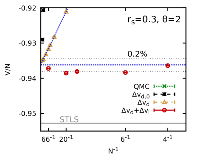
Figure 1: Interaction energy $v$ for $r_{s}=0.3$ and $\theta=2$. Top and bottom: zoomed and full view of $N$-dependence. Green crosses: raw CPIMC Dornheim et al. (2016a) and PIMC data; grey stars: first-order correction $\Delta v^{N}_{\textnormal{d},0}$, Eq. (21); yellow triangles: $\Delta v^{N}_{\textnormal{d}}$, Eq. (II.4); red: $\Delta v^{N}_{\textnormal{d}}+\Delta v^{N}_{\textnormal{i}}$, Eq. (22); dotted blue: linear extrapolation; solid grey: STLS Singwi et al. (1968); Tanaka and Ichimaru (1986); Sjostrom and Dufty (2013).

Let us start our investigation with an example at high density ($r_{s}=0.3$) and extreme temperature ($\theta=2$), which is close to the conditions in the solar core Fortov (2009). In Fig. 1, we show the corresponding dependence of the interaction energy per particle $V^{N}/N$ on the system size $N$. Let us first consider the bottom panel, where we show the entire relevant energy-range. In particular, the green crosses depict the raw, uncorrected QMC data [partly Configuration path integral Monte Carlo (CPIMC) Groth et al. (2016); Dornheim et al. (2016b) data taken from Ref. Dornheim et al. (2016a), and a few data points obtained with standard path integral Monte Carlo (PIMC) Boninsegni et al. (2006a, b); Ceperley (1995)] that have been computed from Eq. (19). Evidently, these data exhibit a strong dependence on $N$ reaching approximately $100\%$ for $N=4$. Even for the largest depicted system size, $N=300$, finite size errors have not completely vanished. The yellow triangles have been obtained by adding to the raw data the FSC for the discretization error using $S^{\textnormal{STLS}}(q)$ as a trial function; see Eq. (II.4) above. This leads to a remarkable reduction of the finite-size errors in the data set, and the residual error appears to be of the order of $\sim 1\%$ even for as few as $N=4$ particles. This validates the previous conclusion from Ref. Dornheim et al. (2016a) that $\Delta v^{N}_{\textnormal{d}}$ does indeed constitute the dominant contribution to the total finite-size error $\Delta v^{N}$. For completeness, we also show the first-order correction $\Delta v^{N}_{\textnormal{d},0}$ [Eq. (21)], which is depicted by the dark grey stars. Yet, this first-order correction is only reasonable for very large numbers of electrons $N$, and even leads to an increase in finite-size errors for $N\lesssim 20$. Finally, the dotted blue line depicts a linear fit to the yellow triangles for $N\geq 20$, which has been used to extrapolate the residual error of these data in Refs. Dornheim et al. (2017a, 2016a, 2018a); Groth et al. (2017b).

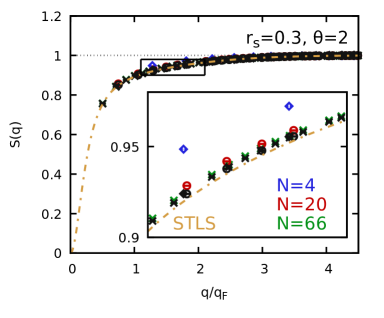
Figure 2: Static structure factor for $r_{s}=0.3$ and $\theta=2$. Coloured symbols depict raw QMC data for $N=66$ (green crosses), $N=20$ (red circles), and $N=4$ (blue diamonds). The corresponding black symbols have been finite-size corrected using Eq. (17). Dash-dotted yellow: STLS Singwi et al. (1968); Tanaka and Ichimaru (1986); Sjostrom and Dufty (2013). Note that $q_{\textnormal{F}}$ denotes the Fermi wave number Giuliani and Vignale (2008).

Let us postpone the discussion of the red circles in Fig. 1, and instead focus on the source of the remaining $N$-dependence after the discretization error has been eliminated. To this end, we show QMC results for the static structure factor in Fig. 2 at the same conditions for three values of $N$. More specifically, the coloured symbols depict the raw, uncorrected QMC results for $S^{N}(q)$ for $N=4$ (blue diamonds), $N=20$ (red circles), and $N=66$ (green crosses). First and foremost, we note that the dependence of $S^{N}(q)$ on $N$ is indeed small when compared to the substantially more pronounced finite-size error of $V^{N}/N$ itself. Still, there do appear significant differences between the data for different $N$, which is particularly pronounced for $N=4$, as it is expected.

Adding the FSC $\Delta S^{N}(q)$ from Eq. (17) to $S^{N}(q)$ leads to the black symbols in Fig. 2. Evidently, this correction works well at these conditions, and the black diamonds, squares, and crosses can hardly be distinguished with the naked eye. This, in turn, means that as few as $N=4$ particles are sufficient to obtain a wave-number resolved description of electronic correlations in the UEG, despite the apparently large finite-size effects at such an extreme density.

Having thus verified our theory for finite-size errors in the static structure factor, we can readily compute the second source of finite-size errors in the interaction energy, namely the intrinsic error $\Delta v^{N}_{\textnormal{i}}$, Eq. (22). The results of removing both intrinsic and discretization errors are depicted by the red circles in Fig. 1. In particular, our new procedure leads to a striking reduction in finite-size errors even for $N=4$ electrons, without any empirical input or knowledge about the behaviour for other $N$. Further, the corrected data for all $N$ are within $\sim 0.2\%$ of the value that was obtained from the extrapolation of the yellow triangles. For comparison, we have also included the prediction for $v$ from STLS Tanaka and Ichimaru (1986); Sjostrom and Dufty (2013) (horizontal grey line) that is obtained by inserting $S^{\textnormal{STLS}}(q)$ in Eq. (18). Even though STLS and related dielectric theories are often considered to be rather accurate at these conditions Dornheim et al. (2020d), we can clearly resolve a systematic overestimation of $v$ by $\sim 1\%$. Yet, this deficiency has no impact on the estimation of $\Delta^{N}_{\textnormal{d}}[S^{\textnormal{STLS}}(q)]$, since the systematic error in $S^{\textnormal{STLS}}(q)$ cancels in Eq. (II.4).

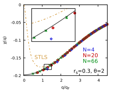
Figure 3: Static density response function $\chi(q)$ for $r_{s}=0.3$ and $\theta=2$. Coloured symbols depict CPIMC data Groth et al. (2017a) for $\chi^{N}_{0}(q)$ for $N=66$ (green crosses), $N=20$ (red circles), and $N=4$ (blue diamonds). Solid black: $\chi^{\textnormal{TDL}}_{0}(q)$; Dash-dotted yellow: STLS Singwi et al. (1968); Tanaka and Ichimaru (1986); Sjostrom and Dufty (2013).

To further illustrate the idea behind our new FSC-scheme, we show the density response function of the corresponding noninteracting (ideal) Fermi system in Fig. 3. In particular, the solid black curve shows $\chi^{\textnormal{TDL}}_{0}(q)$, and the blue diamonds, red circles, and green crosses depict $\chi^{N}_{0}(q)$ for $N=4$, $N=20$, and $N=66$, respectively. Evidently, there appear significant deviations between $\chi^{\textnormal{TDL}}_{0}$ and $\chi_{0}^{N}$ that closely resemble the trend observed in $S^{N}(q)$ shown in Fig. 2 above. In addition, we have also included $\chi^{\textnormal{STLS}}(q)$ in the figure (dash-dotted yellow curve), which serves as a guide to the eye.

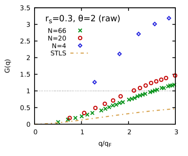
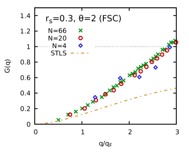
Figure 4: Effective local field correction $\overline{G}^{N}_{\textnormal{invert}}(q)$ for $r_{s}=0.3$ and $\theta=2$, top: raw (uncorrected) results, see Eq. (15); bottom: FSC-corrected data, see Eq. (16).

To conclude our analysis for the present example, we show the actual effectively static local field correction $\overline{G}^{N}_{\textnormal{invert}}(q)$ in Fig. 4 for the same particle numbers. The top panel shows the uncorrected raw data, and we see substantial finite-size effects for all data sets exceeding $100\%$ for $N=4$. The bottom panel shows the corresponding results for $\overline{G}^{\textnormal{FSC}}(q)$ [see Eq. (16)], and we find that the correction $\Delta G^{N}(q)$ defined in Eq. (8) removes nearly the entire dependence on $N$. This finding can be interpreted in the following way: the local field corrections $G(q,0)$ and $\overline{G}_{\textnormal{invert}}(q)$ have been defined as the difference between the exact density response / static structure factor of the system, and the prediction of mean-field theory, i.e., RPA. Therefore, it is a short-range function taking into account exchange–correlation effects, which are hardly affected by the system size at these conditions. Correspondingly, we can accurately extract either $G$ or $\overline{G}_{\textnormal{invert}}$ from a single simulation of the UEG even for $N=4$. Finally, this information about the short-range behaviour can be combined with the mean-field description, thus yielding the full, wave-number resolved description of the system in the TDL.

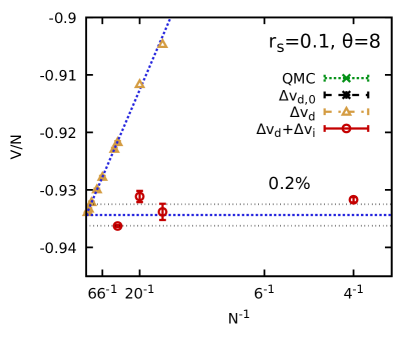
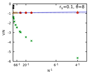
Figure 5: Interaction energy $v$ for $r_{s}=0.1$ and $\theta=8$. Top and bottom: zoomed and full view of $N$-dependence. Green crosses: raw CPIMC and PIMC data; grey stars: first-order correction $\Delta v^{N}_{\textnormal{d},0}$, Eq. (21); yellow triangles: $\Delta v^{N}_{\textnormal{d}}$, Eq. (II.4); red: $\Delta v^{N}_{\textnormal{d}}+\Delta v^{N}_{\textnormal{i}}$, Eq. (22); dotted blue: linear extrapolation;

To discern the limits of our new FSC scheme, we next consider a substantially more extreme case, where even thousands of particles are not sufficient to resemble the TDL. In particular, we show the interaction energy per particle in Fig. 5 for $r_{s}=0.1$ and $\theta=8$. Let us first consider the bottom panel showing the entire relevant energy range of the uncorrected data, which again have been partly taken from Ref. Dornheim et al. (2016a) and computed with CPIMC, and partly obtained using standard PIMC in the context of the present work. The raw QMC results (green crosses) naturally exhibit severe finite-size effects that exceed $500\%$ for $N=4$. Moreover, the dependence of $V^{N}/N$ is substantial even for $N=2000$ (the largest $N$ shown in Fig. 5) and does not follow any obvious functional form. The yellow triangles have again been obtained by removing the discretization error $\Delta v^{N}_{\textnormal{d}}$ estimated using $S^{\textnormal{STLS}}(q)$, which reduces the dependence on $N$ by at least two orders of magnitude. Yet, there still remains a bias of several per cent for the smallest depicted values of $N$. The first-order correction $\Delta v^{N}_{\textnormal{d},0}$, on the other hand, is not appropriate even for $N\sim 10^{3}$ and only becomes accurate for even larger $N$. Finally, the red circles have been computed by subtracting from the yellow triangles the finite-size error due to the intrinsic dependence on $N$ of $S^{N}(q)$, $\Delta v^{N}_{\textnormal{i}}$, computed with our new scheme. Even for this most extreme case, where thousands of particles do not suffice for an appropriate description, we can predict the interaction energy in the TDL with a relative accuracy of $\sim 0.2\%$ from just $N=4$ electrons.

III.2 Increasing the coupling strength

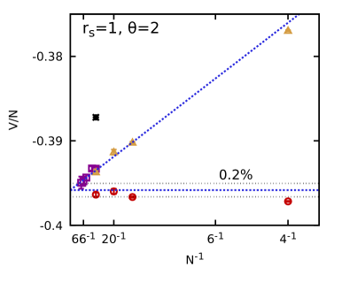
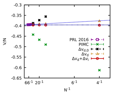
Figure 6: Interaction energy $v$ for $r_{s}=1$ and $\theta=2$. Top and bottom: zoomed and full view of $N$-dependence. Green crosses: raw PIMC data; grey stars: first-order correction $\Delta v^{N}_{\textnormal{d},0}$, Eq. (21); yellow triangles: $\Delta v^{N}_{\textnormal{d}}$, Eq. (II.4); red: $\Delta v^{N}_{\textnormal{d}}+\Delta v^{N}_{\textnormal{i}}$, Eq. (22); dotted blue: linear extrapolation; purple squares: PB-PIMC Dornheim et al. (2015a, b) data corrected with $\Delta v^{N}_{\textnormal{d}}$ taken from Ref. Dornheim et al. (2016a).

To further assess the remarkable performance of our new FSC scheme demonstrated at high densities in the previous section, we will now investigate the manifestation of finite-size effects upon increasing the density parameter $r_{s}$. For a quantum system such as the UEG, this is equivalent to increasing the coupling strength, see e.g. Refs. Giuliani and Vignale (2008); Ott et al. (2018). A first example is shown in Fig. 6, where we plot the interaction energy per particle for $r_{s}=1$ and $\theta=2$. First and foremost, we find that finite-size errors are overall reduced in magnitude compared to $r_{s}=0.3$ shown in Fig. 1 above, as it is expected. In addition, the discretization error again accounts for the bulk of finite-size effects, as the yellow triangles constitute a substantial improvement over the green crosses. Further, the purple squares taken from Ref. Dornheim et al. (2016a) have been obtained using the Permutation blocking PIMC (PB-PIMC) method Dornheim et al. (2015a, b, 2017b, 2019b) and, too, were corrected using $\Delta v^{N}_{\textnormal{d}}[S^{\textnormal{STLS}}(q)]$. These data are in excellent agreement to the independent standard PIMC data obtained for the present work, which further corroborates the high quality of the existing description of the UEG Groth et al. (2017b); Dornheim et al. (2018a). At the same time, the first-order correction $\Delta v^{N}_{\textnormal{d},0}$ is not sufficiently accurate to replace the full evaluation of Eq. (II.4). Finally, the new FSC-scheme for the intrinsic error $\Delta v^{N}_{\textnormal{i}}$ results in the red circles, where the residual error does not exceed $\sim 0.3\%$ even for $N=4$.

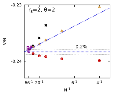
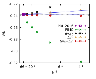
Figure 7: Interaction energy $v$ for $r_{s}=2$ and $\theta=2$. Top and bottom: zoomed and full view of $N$-dependence. Green crosses: raw PIMC data; grey stars: first-order correction $\Delta v^{N}_{\textnormal{d},0}$, Eq. (21); yellow triangles: $\Delta v^{N}_{\textnormal{d}}$, Eq. (II.4); red circles: $\Delta v^{N}_{\textnormal{d}}+\Delta v^{N}_{\textnormal{i}}$, Eq. (22); dotted blue: linear extrapolation; purple squares: PB-PIMC Dornheim et al. (2015a, b) data corrected with $\Delta v^{N}_{\textnormal{d}}$ taken from Ref. Dornheim et al. (2016a).

Let us next further increase the density parameter to $r_{s}=2$, which is shown in Fig. 7. This is a typical density for the conduction band electrons in metals, and thus such a case is of paramount importance. In warm dense matter research, such states are created in many experiments, e.g. using aluminum Sperling et al. (2015); Sprösser-Prou et al. (1989); Takada and Yasuhara (2002); Ramakrishna et al. (2020). In this case, finite-size effects are again reduced in relative importance, and the first-order correction from Eq. (21) becomes accurate for $N\sim 34$. Yet, there still remain significant residual errors in $V/N$ after the discretization error is removed, which are of the order of a few per cent for $N=4$ and decrease to $\sim 0.5\%$ for $N=20$. While it is certainly feasible to carry out a controlled extrapolation of the remaining $N$-dependence of the data at these conditions, it is still worth investigating if our new scheme makes this effort superfluous.

Thus, we have added our estimation of $\Delta v^{N}_{\textnormal{i}}$ to the yellow triangles, and the results are as usual depicted by the red circles. We find that our scheme significantly reduces the dependence on $N$ for all numbers of electrons, although the actual error seems to be overestimated by Eq. (22). For example, the thus fully corrected value for the interaction energy per particle for $N=4$ deviates by almost $1\%$ from the extrapolated result (horizontal dotted blue line), and these residual deviations decrease with increasing $N$. We thus conclude that our new scheme does indeed constitute an improvement over the previous state-of-the-art of FSCs, but the finite-size error cannot be completely removed for $N=4$.

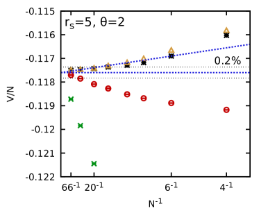
Figure 8: $N$-dependence of the interaction energy $v$ for $r_{s}=5$ and $\theta=2$. Green crosses: raw PIMC data; grey stars: first-order correction $\Delta v^{N}_{\textnormal{d},0}$, Eq. (21); yellow triangles: $\Delta v^{N}_{\textnormal{d}}$, Eq. (II.4); red circles: $\Delta v^{N}_{\textnormal{d}}+\Delta v^{N}_{\textnormal{i}}$, Eq. (22); dotted blue: linear extrapolation; solid grey: STLS Singwi et al. (1968); Tanaka and Ichimaru (1986); Sjostrom and Dufty (2013).

In order to understand this observed trend, it makes sense to go to even larger values of the coupling strength. To this end, we show the interaction energy per particle for $r_{s}=5$ and $\theta=2$ in Fig. 8. We note that such a low density serves a valuable laboratory for the impact of electronic exchange–correlation effects on material properties Mazevet et al. (2005); Desjarlais et al. (2002) and can be realized experimentally for example via hydrogen jets Zastrau et al. (2014). First and foremost, we observe a further reduced relative magnitude of finite-size effects, as can be seen by the green crosses depicting the raw PIMC data for $N\geq 20$. Moreover, both the full expression for $\Delta v_{\textnormal{d}}^{N}$ and the first-order term $\Delta v_{\textnormal{d},0}^{N}$ give fairly similar results and are all but indistinguishable for $N\gtrsim 10$. Moreover, the residual error after removing the discretization error does not exceed $0.3\%$ in this case. Finally, the red circles have been obtained by further adding to the yellow triangles the result for $\Delta v^{N}_{\textnormal{i}}$. Evidently, Eq. (22) substantially overestimates true residual error and, in fact, exhibits an even somewhat more pronounced and less trivial dependence on $N$. The rest of this section will attempt to explain this unexpected break down of our expression for $\Delta v^{N}_{\textnormal{i}}$ in some detail.

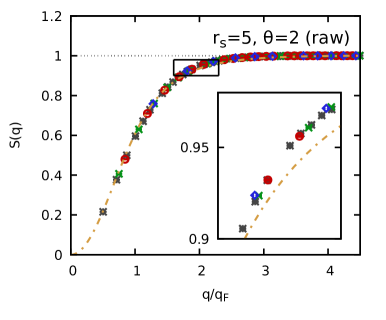
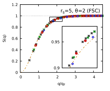
Figure 9: Static structure factor $S(q)$ for $r_{s}=5$ and $\theta=2$. The top and bottom panels show raw, uncorrected PIMC data for $S^{N}(q)$ and the corrected $S^{N}_{\textnormal{FSC}}(q)$ [see Eq. (17)], respectively. Blue diamonds: $N=4$; red circles: $N=14$; green crosses: $N=20$; grey stars: $N=66$. Dash-dotted yellow: STLS Tanaka and Ichimaru (1986); Sjostrom and Dufty (2013).

Let us begin this analysis by considering the central ingredient to the interaction energy, i.e., the static structure factor $S(q)$ shown in Fig. 9. The top panel shows standard PIMC results for the raw, uncorrected $S^{N}(q)$ for $N=4$ (blue diamonds), $N=14$ (red circles), $N=20$ (green crosses), and $N=66$ (grey stars). In addition, the dash-dotted yellow curve corresponds to $S^{\textnormal{STLS}}(q)$ and has been included as a reference. Interestingly, the only substantial intrinsic dependence of $S^{N}(q)$ on $N$ appears for $N=4$, whereas the other data seem to fall on a continuous curve.

The bottom panel of the same figure shows the same information, but for the finite-size corrected version of the SSF, $S^{N}_{\textnormal{FSC}}(q)$. In this case, we find that adding our expression for $\Delta S^{N}(q)$ from Eq. (17) onto $S^{N}(q)$ leads to a substantial increase of finite-size effects and we find a significant difference even between $N=20$ and $N=66$ that was absent in the top panel. We have thus found, that our new scheme for the FSC for $v$ breaks down, because the involved expression for $\Delta S^{N}(q)$ becomes inappropriate.

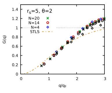
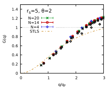
Figure 10: Top: Effective local field correction $\overline{G}^{N}_{\textnormal{invert}}(q)$ (top panel) and static limit $G^{N}(q,0)$ (bottom panel) for $r_{s}=5$ and $\theta=2$; coloured symbols: raw (uncorrected) results, see Eqs. (15) and (6), black: FSC-corrected, using Eq. (8). Dash-dotted yellow: LFC from STLS Tanaka and Ichimaru (1986); Sjostrom and Dufty (2013).

Proceeding to the next deeper level of explanation, we show different local field corrections in Fig. 10 for the same conditions. The top panel corresponds to the effectively static local field correction $\overline{G}_{\textnormal{invert}}(q)$ defined in Eq. (15) above, and the blue diamonds, red circles, and green crosses show the raw, uncorrected data for $N=4$, $N=14$, and $N=20$, respectively. In addition, the dash-dotted yellow line shows the LFC from STLS and has been included as a reference. Similar to our previous observation regarding $S^{N}(q)$ above, here, too, we only find small finite-size effects for $N=4$, and no dependence on $N$ is visible for $N=14$ and $N=20$. The black symbols in the same panel have been obtained by adding to $\overline{G}^{N}_{\textnormal{invert}}(q)$ the finite-size correction for the static LFC $G^{N}(q,0)$, $\Delta G^{N}(q)$, given in Eq. (8). Again, the FSC exacerbates the actual $N$-dependence of the uncorrected data.

This can potentially be explained by two distinctly different effects: i) the FSC for the static LFC $G^{N}(q,0)$ could be fundamentally different to the real, a-priori unknown FSC for $\overline{G}^{N}_{\textnormal{invert}}(q)$, or ii) our expression for $\Delta G^{N}(q)$ is inappropriate for both $G^{N}(q,0)$ and $\overline{G}^{N}_{\textnormal{invert}}(q)$. This question is resolved by the analysis presented in the bottom panel of Fig. 10, where we show the exact static limit of the LFC for the same conditions as in the top panel. Evidently, the different data for $G(q,0)$ exhibit the same trend as $\overline{G}_{\textnormal{invert}}^{N}(q)$. In particular, the FSC $\Delta G^{N}(q)$ does not constitute an improvement over the uncorrected PIMC data, which means that explanation ii) holds: we do not have an appropriate theory for finite-size effects in both $G^{N}(q,0)$ and $\overline{G}_{\textnormal{invert}}^{N}(q)$ at these conditions.

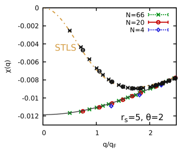
Figure 11: Static density response function for $r_{s}=5$ and $\theta=2$. Green crosses, red circles, and blue diamonds: $\chi^{N}_{0}(q)$ for $N=4$, $N=20$, and $N=66$, respectively. The corresponding black symbols show PIMC results for $\chi^{N}(q)$ evaluated from Eq. (3). Solid grey: $\chi^{\textnormal{TDL}}_{0}(q)$; Dash-dotted yellow: $\chi^{\textnormal{STLS}}(q)$ Tanaka and Ichimaru (1986); Sjostrom and Dufty (2013).

This can be understood more intuitively by examining Fig. 11, where we show data for different density response functions $\chi(q)$. More specifically, The coloured symbols depict the results for $\chi_{0}^{N}(q)$, and the solid dark grey curve depicts $\chi^{\textnormal{TDL}}_{0}(q)$. We note that there are substantial finite-size effects, in particular for $N=4$, as it is expected. In contrast, the black symbols depict the static density response function of the UEG that was computed using standard PIMC via Eq. (3), and no dependence on $N$ can be resolved with the bare eye. We have thus found that finite-size effects in the actual density response function $\chi^{N}(q)$ [and also in $S^{N}(q)$] disappear with increasing $r_{s}$, which does not hold for $\chi_{0}^{N}(q)$. Yet, if it is $\chi^{N}(q)\approx\chi^{\textnormal{TDL}}(q)$, then using $\chi^{\textnormal{TDL}}_{0}(q)$ in Eq. (6) is actually consistent and directly leads to the static local field correction in the TDL, $G^{N}(q)\approx G^{\textnormal{TDL}}(q)$, just as we have observed in Fig. 10.

The spurious effects of the finite-size correction $\Delta^{N}G(q)$ can then finally be interpreted in the following way: The mean-field description that is directly based on $\chi_{0}^{N}(q)$ predicts substantial finite-size effects. These, however, are absent from the actual density response function $\chi^{N}(q)$ which we computed via PIMC. Therefore, we can conclude that the system-size dependence is suppressed by the increased coupling strength, since the particles are considerably more localized due to the Coulomb repulsion. It is then only meaningful to define the LFC as the difference between $\chi_{0}^{\textnormal{TDL}}(q)$ and $\chi^{N}(q)$, as the finite-size effects in $\chi^{N}_{0}(q)$ do not manifest in the latter. If we instead would define $G^{N}(q,0)$ as the difference between $\chi^{N}(q)$ and $\chi_{0}^{N}(q)$, this LFC would have to balance the system-size dependence from $\chi^{N}_{0}(q)$, so that the actual density response function remains independent of $N$. This then explains the unreasonable behaviour of $\Delta G^{N}(q)$ shown in Fig. 10.

In a nutshell, our new FSC scheme implicitly assumes that the description of the system can be decomposed into a mean-field part that exhibits finite-size effects, and a short-range LFC that does not. At large values of $r_{s}$, this assumption breaks down, as the finite-size effects in $\chi^{N}_{0}(q)$ are suppressed by the strong Coulomb repulsion. At the same time, we note that this is not catastrophic, as the dependence of QMC data on $N$ is small for lower densities in the first place Dornheim et al. (2016a, 2018a).

III.3 Going to low temperature

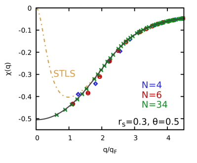
Figure 12: Density response functions for $\theta=0.5$ and $r_{s}=0.3$. The blue diamonds, red circles, and green crosses correspond to $\chi^{N}_{0}(q)$ for $N=4$, $N=6$, and $N=34$, respectively. Dark grey solid line: $\chi^{\textnormal{TDL}}_{0}(q)$; dash-dotted yellow: $\chi^{\textnormal{STLS}}(q)$, see Refs. Tanaka and Ichimaru (1986); Sjostrom and Dufty (2013).

The final part of the investigation in this work is devoted to the performance of our new FSC scheme for low temperatures. This is a particularly interesting regime, as accurate QMC data for the UEG are sparse at these conditions due to the fermion sign problem Dornheim (2019); Lee et al. (2020); Yilmaz et al. (2020); Dornheim et al. (2017a). In addition, the UEG has attracted renewed interest at high densities also in the ground-state Shepherd et al. (2012a, b), where the full configuration interaction QMC (FCIQMC) method Booth et al. (2009) is capable to give accurate results for finite $N$.

One of the main sources of finite-size errors at low temperature is given by momentum-shell effects. For this reason, one typically selects a system-size that is commensurate to the grid in momentum space, e.g. for an unpolarized UEG $N=14,38,54,66,\dots$. An additional strategy is to employ periodic boundary conditions with a finite twist-angle Lin et al. (2001); Zong et al. (2002); Sorella (2015); Azadi and Foulkes (2019); Mihm et al. (2019) and perform a subsequent twist-averaging which has been shown to greatly alleviate these effects. At the same time, we note that these momentum shell effects are already fully present in $\chi^{N}_{0}(q)$, which makes our new FSC promising in this regime. This is illustrated in Fig. 12, where we show the density response function for $r_{s}=0.3$ and $\theta=0.5$. Here, the blue diamonds, red circles, and green crosses show $\chi_{0}^{N}(q)$ for $N=4$, $N=6$, and $N=34$, respectively, and the solid dark grey curve corresponds to $\chi^{\textnormal{TDL}}_{0}(q)$. In addition, the dash-dotted curve shows $\chi^{\textnormal{STLS}}(q)$ and has been included as a reference. Firstly, we note that $\theta=0.5$ only constitutes the boundary of the low-temperature regime, and thermal excitations still play an important role Dornheim et al. (2018a). Still, incipient momentum shell effects clearly manifest for $\chi_{0}^{N}(q)$ in Fig. 12, in particular for $N=4$. Similar results for lower temperatures have been presented by Groth et al. Groth et al. (2017a).

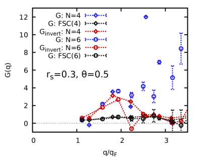
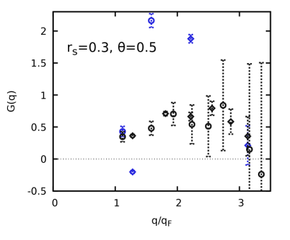
Figure 13: Different local field corrections for $\theta=0.5$ and $r_{s}=0.3$. The diamonds and circles correspond to $N=4$ and $N=6$ electrons. Blue: raw, uncorrected static LFC $G^{N}(q,0)$, see Eq. (6); black: $G^{\textnormal{FSC}}_{N}(q)$ using Eq. (8); red: raw, uncorrected results for $\overline{G}^{N}_{\textnormal{invert}}(q)$, see Eq. (15). Bottom panel: magnified view around the corrected values $G^{\textnormal{FSC}}_{N}(q)$ from the top panel.

The next step towards a finite-size correction for $S^{N}(q)$ and $V^{N}/N$ is given by analysis of different local field corrections presented in Fig. 13 for the same conditions. Let us first consider the top panel where we show results for $N=4$ (diamonds) and $N=6$ (circles). The red data show $\overline{G}_{\textnormal{invert}}^{N}(q)$, which constitutes the basis of our FSC scheme for $\Delta S^{N}(q)$ and, in turn, $\Delta v^{N}_{\textnormal{i}}$. Apparently, the data sets for the two different particle numbers do not follow a smooth progression, and a finite-size correction is needed; similarly, $S^{N}(q)$ exhibits finite-size effects, see the discussion of Fig. 14 below. The blue data show results for the static limit of the LFC $G^{N}(q,0)$ and have been obtained from PIMC simulations via Eq. (3) and Eq. (6). On the one hand, these data, too, do exhibit substantial finite-size effects, which further underlines the need for an FSC. On the other hand, the system-size dependence of $G^{N}(q)$ does not resemble the observed behaviour of $\overline{G}^{N}_{\textnormal{invert}}(q)$, which makes the applicability of our FSC scheme questionable.

Remarkably, adding the FSC $\Delta G^{\textnormal{FSC}}(q)$ to the blue points gives the black curves, for which no dependence on $N$ can be resolved within the given level of statistical uncertainty. This can be seen particularly well in the bottom panel where we show a magnified view around $G^{\textnormal{FSC}}_{N}(q)$. Thus, QMC simulations of $N=4$ and $N=6$ electrons appear to give us access to $G(q,0)$ in the TDL, but not $\overline{G}^{\textnormal{TDL}}_{\textnormal{invert}}(q)$ as no theory for $\Delta\overline{G}^{N}_{\textnormal{invert}}(q)$ is at hand.

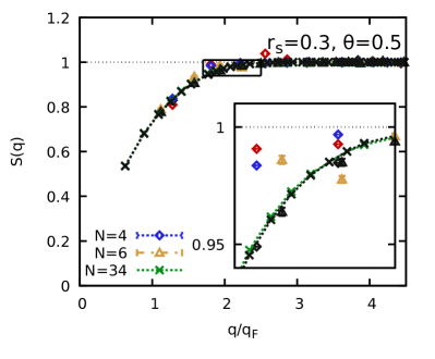
Figure 14: SSF for $\theta=0.5$ and $r_{s}=0.3$. Green crosses: raw CPIMC data for $N=34$ taken from Ref. Dornheim et al. (2016a); blue diamonds: raw PIMC data for $N=4$; yellow triangles: raw PIMC data for $N=6$; the corresponding black symbols have been finite-size corrected, for $N=34$ in the regular way [Eq. (17)], for $N=4,6$ with Eq. (25); red diamonds: static approximation using $G^{N}(q,0)$ for $N=4$.

Let us next ponder the consequences of these findings for the FSC of the static structure factor $S(q)$, which we show in Fig. 14 for the same conditions. Here the blue diamonds, yellow triangles and green crosses show the raw, uncorrected QMC data for $S^{N}(q)$. We note that the observed dependence on $N$ is qualitatively similar to the finite-size effects observed in $\chi_{0}^{N}(q)$ in Fig. 12 above. In addition, the red diamonds have been obtained by using $G^{N}(q,0)$ to compute the static structure factor within the static approximation [Eq. (14)]. Evidently, these data do substantially disagree with the actual QMC data for $S^{N}(q)$, which appears to indicate that the static approximation is not applicable at these conditions. This is not surprising and directly explains the difference between $\overline{G}^{N}_{\textnormal{invert}}(q)$ and $G^{N}(q)$ in Fig. 13.

Yet, the full picture is even more subtle and can be deduced from the black diamonds in Fig. 14, which show the static structure factor $S^{\textnormal{FSC}}_{\textnormal{stat}}(q)$ obtained via the static approximation using as input the finite-size corrected LFC $G^{\textnormal{FSC}}_{N}(q)$ for $N=4$. Remarkably, these data do not exhibit the unsmooth behaviour of $S^{N}(q)$ associated with the momentum shell effects, but for a smooth progression with $q$. Moreover, these data are much closer to the green crosses depicting the QMC data for $N=34$, and the black crosses, that have been obtained by applying the usual FSC $\Delta S^{N}(q)$ [Eq. (17)] to the latter.

These findings indicate that the static approximation does not break down at these conditions after all, since the black diamonds appear to be accurate. Instead, the large discrepancy between the blue and red diamonds follows from an inconsistent mixing of different response functions, which did not matter for $\theta=2$, but has a large impact in the low temperature regime. More specifically, a consistent static approximation for a finite number of electrons $N$ should have the form

$$\chi^{N}_{\textnormal{stat}}(q,\omega)=\frac{\chi^{N}_{0}(q,\omega)}{1-\frac{4\pi}{q^{2}}\left[1-G^{N}(q)\right]\chi^{N}_{0}(q,\omega)}\ ,$$ (24)

where the dynamic density response function of the ideal Fermi gas is computed for the same system size. Thus, combining $G^{\textnormal{FSC}}_{N}(q)$ with $\chi^{\textnormal{TDL}}_{0}(q,\omega)$ gives reasonable results for $S(q)$ (black diamonds), whereas mixing $G^{N}(q)$ with $\chi^{\textnormal{TDL}}_{0}(q,\omega)$ does neither fit to the TDL, nor the QMC data for $S^{N}(q)$. Following this line of thinking, our definition of $\overline{G}_{\textnormal{invert}}^{N}(q)$ from Eq. (15) above, too, is inconsistent, as it must reproduce $S^{N}(q)$ using the inappropriate TDL result $\chi^{\textnormal{TDL}}_{0}(q,\omega)$. Instead, one should define a modified effective LFC, where the functional $S[\overline{G}(q)](q)$ is evaluated using the static approximation from Eq. (24). The implementation of this idea, however, is beyond the scope of the present work and constitutes a project for future research.

The final question to be discussed here is whether it is still possible to compute a reasonable estimation for the intrinsic contribution to the finite-size error of the interaction energy $\Delta v^{N}_{\textnormal{i}}$ without detailed knowledge of $\chi^{N}_{0}(q,\omega)$. This is indeed possible, as we do have access to finite-size corrected data for $S(q)$ in the form of the black diamonds in Fig. 14 that have been obtained from the static approximation using as input $G^{\textnormal{FSC}}_{N}(q)\approx G^{\textnormal{TDL}}(q)$. From these, we can deduce an approximate expression for the finite-size effects in $S^{N}(q)$ as

$$\Delta S^{N}_{\textnormal{stat}}(q)=S^{\textnormal{FSC}}_{\textnormal{stat}}(q)-S^{N}(q)\ .$$ (25)

In particular, we stress that Eq. (25) cannot be exact, as $S^{\textnormal{FSC}}_{\textnormal{stat}}(q)$ entails the (small) systematic error from the static approximation [i.e., neglecting the frequency-dependence of the full LFC $G(q,\omega)$], which is absent from $S^{N}(q)$. Still, we stress that this systematic bias is small, especially at the high densities that are of interest to the present work Dornheim et al. (2018b); Hamann et al. (2020), and that Eq. (25) is only used to estimate the small correction to the interaction energy per particle, and not $V^{N}/N$ itself. The corresponding expression for the intrinsic contribution to $\Delta v^{N}$ is then given by

$$\Delta v_{\textnormal{i}}^{N}[\textnormal{stat}]=\frac{1}{2V}\sum_{\mathbf{G}\neq\mathbf{0}}\left[S_{\textnormal{stat}}^{\textnormal{FSC}}(\mathbf{G})-S^{N}(\mathbf{G})\right]\frac{4\pi}{G^{2}}\ .$$ (26)

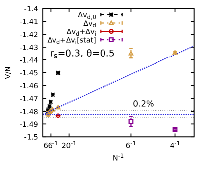
Figure 15: Interaction energy $v$ for $r_{s}=0.3$ and $\theta=0.5$. Green crosses: raw CPIMC and PIMC data; grey stars: first-order correction $\Delta v^{N}_{\textnormal{d},0}$, Eq. (21); yellow triangles: $\Delta v^{N}_{\textnormal{d}}$, Eq. (II.4); red circles: $\Delta v^{N}_{\textnormal{d}}+\Delta v^{N}_{\textnormal{i}}$, Eq. (22); dotted blue: linear extrapolation; purple squares: adapted FSC $\Delta v^{N}_{\textnormal{d}}+\Delta v^{N}_{\textnormal{i}}[\textnormal{stat}]$, see Eq. (26).

Let us conclude our investigation of finite-size effects in electronic structure simulations at extreme conditions with an analysis of the interaction energy shown in Fig. 15. In particular, we only show a magnified segment around the finite-size corrected data sets, as the overall trend is quite similar to the case of $\theta=2$ shown in Fig. 1 above. Further, the zero-order expression $\Delta v_{\textnormal{d},0}^{N}$ from Eq. (21) only becomes appropriate for large $N$, and the full estimation of $\Delta v_{\textnormal{d}}^{N}$ is needed. Still, there remains a significant residual error that only vanishes within the given Monte Carlo error bars for $N\gtrsim 66$. Using Eq. (26) to estimate the intrinsic error in $v$ gives the purple squares, where the residual error is reduced by nearly an order of magnitude. We thus conclude that accurate knowledge of the static response functions $\chi^{N}(q)$ and $\chi_{0}^{N}(q)$ can be used in lieu of the full frequency-dependence of $\chi^{N}_{0}(q,\omega)$ to compute a reasonable estimate of $\Delta v_{\textnormal{i}}^{N}$ within the static approximation at low temperatures.

IV Summary and Outlook

IV.1 Summary

In summary, we have presented a FSC scheme for the static structure factor $S(q)$ and, in this way, also the interaction energy per particle $v$. More specifically, we have employed the density response formalism and identified an effectively frequency-averaged static local field correction $\overline{G}_{\textnormal{invert}}(q)$ as a short-ranged exchange–correlation property that can be extracted from a QMC simulation of only a few particles.

As a practical application, we have investigated the UEG at extreme conditions Dornheim et al. (2018a) and demonstrated that often as few as $N=4$ electrons are sufficient to obtain the interaction energy with a relative accuracy of $\sim 0.2\%$. We stress that our approach is completely nonempirical, and does not require any external input or simulation data for different $N$.

In addition, we have analyzed the applicability of our scheme upon increasing the density parameter $r_{s}$ (and thus the coupling strength), and found that it eventually breaks down when correlation effects dominate. Finally, we have investigated the UEG at low temperature, where momentum shell effects constitute an additional source of finite-size errors. Still, these errors, too, are present in the density response function of the noninteracting system $\chi^{N}_{0}(q)$, and we have outlined two different strategies to mitigate the $N$-dependence in this case: i) knowledge of the static interacting response function $\chi^{N}(q)$ allows to obtain an accurate (though not exact) FSC for both $S(q)$ and $v$ which reduces the residual error in $v$ after the elimination of the discretization error by an additional order of magnitude, and ii) using $\chi^{N}_{0}(q,\omega)$ would allow to construct a consistent, $N$-dependent implementation of the static approximation, which has the potential to fully remove momentum shell effects and, in this way, remove the need for an additional twist-averaging procedure.

IV.2 Outlook

We believe that our findings open new avenues for additional topics of research to be pursued in future investigations. First and foremost, we call to mind the direct relation between $S(q)$ and the pair distribution function $g(r)$, which can be exploited to derive a FSC for the latter. In particular, this could be vital for the determination of $g(0)$, which has most recently been investigated by Hunger et al. Hunger et al. (2021) and is important for different applications, e.g. Refs. Dornheim et al. (2020e); Dornheim and Moldabekov (2021). In addition, the idea behind $S(q)$ can be straightforwardly extended to the imaginary-time density–density correlation function $F(q,\tau)$ defined in Eq. (4) above. This function is of high value, as it allows for the computation of the dynamic structure factor $S(q,\omega)$ and related properties Dornheim et al. (2018b); Groth et al. (2019); Hamann et al. (2020), which, in turn, are accessible in experiments, e.g. using the X-ray Thomson scattering technique Glenzer and Redmer (2009); Kraus et al. (2019). Furthermore, we mention the well-known thermodynamic relations between different energies, e.g. Eq. (13), which potentially allow to generalize our correction for $v$ to other quantities such as the kinetic energy. Finally, we point out that our method is particularly successful for high temperatures and densities, which indicates that it may apply to classical molecular dynamics simulations Mithen et al. (2012); Kählert (2020); Ott et al. (2012) as well.

References

- Giuliani and Vignale (2008) G. Giuliani and G. Vignale, Quantum Theory of the Electron Liquid (Cambridge University Press, Cambridge, 2008).
- Burke (2012) Kieron Burke, “Perspective on density functional theory,” The Journal of Chemical Physics 136, 150901 (2012), https://doi.org/10.1063/1.4704546 .
- Jones (2015) R. O. Jones, “Density functional theory: Its origins, rise to prominence, and future,” Rev. Mod. Phys. 87, 897–923 (2015).
- Booth et al. (2013) George H. Booth, Andreas Grüneis, Georg Kresse, and Ali Alavi, “Towards an exact description of electronic wavefunctions in real solids,” Nature 493, 365–370 (2013).
- Anderson (2007) J.B. Anderson, Quantum Monte Carlo: Origins, Development, Applications (Oxford University Press, USA, 2007).
- Ceperley and Alder (1980) D. M. Ceperley and B. J. Alder, “Ground state of the electron gas by a stochastic method,” Phys. Rev. Lett. 45, 566–569 (1980).
- Perdew and Wang (1992) John P. Perdew and Yue Wang, “Accurate and simple analytic representation of the electron-gas correlation energy,” Phys. Rev. B 45, 13244–13249 (1992).
- Perdew and Zunger (1981) J. P. Perdew and Alex Zunger, “Self-interaction correction to density-functional approximations for many-electron systems,” Phys. Rev. B 23, 5048–5079 (1981).
- Vosko et al. (1980) S. H. Vosko, L. Wilk, and M. Nusair, “Accurate spin-dependent electron liquid correlation energies for local spin density calculations: a critical analysis,” Canadian Journal of Physics 58, 1200–1211 (1980), https://doi.org/10.1139/p80-159 .
- Perdew et al. (1996) John P. Perdew, Kieron Burke, and Matthias Ernzerhof, “Generalized gradient approximation made simple,” Phys. Rev. Lett. 77, 3865–3868 (1996).
- Loh et al. (1990) E. Y. Loh, J. E. Gubernatis, R. T. Scalettar, S. R. White, D. J. Scalapino, and R. L. Sugar, “Sign problem in the numerical simulation of many-electron systems,” Phys. Rev. B 41, 9301–9307 (1990).
- Troyer and Wiese (2005) M. Troyer and U. J. Wiese, “Computational complexity and fundamental limitations to fermionic quantum Monte Carlo simulations,” Phys. Rev. Lett 94, 170201 (2005).
- Dornheim (2019) T. Dornheim, “Fermion sign problem in path integral Monte Carlo simulations: Quantum dots, ultracold atoms, and warm dense matter,” Phys. Rev. E 100, 023307 (2019).
- Fraser et al. (1996) Louisa M. Fraser, W. M. C. Foulkes, G. Rajagopal, R. J. Needs, S. D. Kenny, and A. J. Williamson, “Finite-size effects and coulomb interactions in quantum monte carlo calculations for homogeneous systems with periodic boundary conditions,” Phys. Rev. B 53, 1814–1832 (1996).
- Kent et al. (1999) P. R. C. Kent, Randolph Q. Hood, A. J. Williamson, R. J. Needs, W. M. C. Foulkes, and G. Rajagopal, “Finite-size errors in quantum many-body simulations of extended systems,” Phys. Rev. B 59, 1917–1929 (1999).
- Williamson et al. (1997) A. J. Williamson, G. Rajagopal, R. J. Needs, L. M. Fraser, W. M. C. Foulkes, Y. Wang, and M.-Y. Chou, “Elimination of coulomb finite-size effects in quantum many-body simulations,” Phys. Rev. B 55, R4851–R4854 (1997).
- Lin et al. (2001) C. Lin, F. H. Zong, and D. M. Ceperley, “Twist-averaged boundary conditions in continuum quantum monte carlo algorithms,” Phys. Rev. E 64, 016702 (2001).
- Chiesa et al. (2006) Simone Chiesa, David M. Ceperley, Richard M. Martin, and Markus Holzmann, “Finite-size error in many-body simulations with long-range interactions,” Phys. Rev. Lett. 97, 076404 (2006).
- Chiesa et al. (2007) Simone Chiesa, D. M. Ceperley, R. M. Martin, and Markus Holzmann, “Random phase approximation and the finite size errors in many body simulations,” AIP Conference Proceedings 918, 284–288 (2007), https://aip.scitation.org/doi/pdf/10.1063/1.2751996 .
- Azadi and Foulkes (2019) Sam Azadi and W. M. C. Foulkes, “Efficient method for grand-canonical twist averaging in quantum monte carlo calculations,” Phys. Rev. B 100, 245142 (2019).
- Mihm et al. (2019) Tina N. Mihm, Alexandra R. McIsaac, and James J. Shepherd, “An optimized twist angle to find the twist-averaged correlation energy applied to the uniform electron gas,” The Journal of Chemical Physics 150, 191101 (2019), https://doi.org/10.1063/1.5091445 .
- Holzmann et al. (2016) Markus Holzmann, Raymond C. Clay, Miguel A. Morales, Norm M. Tubman, David M. Ceperley, and Carlo Pierleoni, “Theory of finite size effects for electronic quantum monte carlo calculations of liquids and solids,” Phys. Rev. B 94, 035126 (2016).
- Holzmann et al. (2011a) Markus Holzmann, Bernard Bernu, and David M Ceperley, “Finite-size analysis of the fermi liquid properties of the homogeneous electron gas,” Journal of Physics: Conference Series 321, 012020 (2011a).
- Drummond et al. (2008) N. D. Drummond, R. J. Needs, A. Sorouri, and W. M. C. Foulkes, “Finite-size errors in continuum quantum monte carlo calculations,” Phys. Rev. B 78, 125106 (2008).
- Holzmann et al. (2011b) Markus Holzmann, Bernard Bernu, Carlo Pierleoni, Jeremy McMinis, David M. Ceperley, Valerio Olevano, and Luigi Delle Site, “Momentum distribution of the homogeneous electron gas,” Phys. Rev. Lett. 107, 110402 (2011b).
- Dornheim et al. (2016a) T. Dornheim, S. Groth, T. Sjostrom, F. D. Malone, W. M. C. Foulkes, and M. Bonitz, “Ab initio quantum Monte Carlo simulation of the warm dense electron gas in the thermodynamic limit,” Phys. Rev. Lett. 117, 156403 (2016a).
- Dornheim et al. (2018a) T. Dornheim, S. Groth, and M. Bonitz, “The uniform electron gas at warm dense matter conditions,” Phys. Reports 744, 1–86 (2018a).
- Moroni et al. (1995) S. Moroni, D. M. Ceperley, and G. Senatore, “Static response and local field factor of the electron gas,” Phys. Rev. Lett 75, 689 (1995).
- Kwee et al. (2008) Hendra Kwee, Shiwei Zhang, and Henry Krakauer, “Finite-size correction in many-body electronic structure calculations,” Phys. Rev. Lett. 100, 126404 (2008).
- Buraczynski et al. (2018) M. Buraczynski, W. Dawkins, N. Ismail, and A. Gezerlis, “Exploring finite-size effects in strongly correlated systems,” in European Physical Journal Web of Conferences, European Physical Journal Web of Conferences, Vol. 182 (2018) p. 02044.
- Spink et al. (2013) G. G. Spink, R. J. Needs, and N. D. Drummond, “Quantum monte carlo study of the three-dimensional spin-polarized homogeneous electron gas,” Phys. Rev. B 88, 085121 (2013).
- Brown et al. (2013) Ethan W. Brown, Bryan K. Clark, Jonathan L. DuBois, and David M. Ceperley, “Path-integral monte carlo simulation of the warm dense homogeneous electron gas,” Phys. Rev. Lett. 110, 146405 (2013).
- Groth et al. (2017a) S. Groth, T. Dornheim, and M. Bonitz, “Configuration path integral Monte Carlo approach to the static density response of the warm dense electron gas,” J. Chem. Phys 147, 164108 (2017a).
- Foulkes et al. (2001) W. M. C. Foulkes, L. Mitas, R. J. Needs, and G. Rajagopal, “Quantum monte carlo simulations of solids,” Rev. Mod. Phys. 73, 33–83 (2001).
- Bonitz et al. (2020) M. Bonitz, T. Dornheim, Zh. A. Moldabekov, S. Zhang, P. Hamann, H. Kählert, A. Filinov, K. Ramakrishna, and J. Vorberger, “Ab initio simulation of warm dense matter,” Physics of Plasmas 27, 042710 (2020), https://doi.org/10.1063/1.5143225 .
- Graziani et al. (2014) F. Graziani, M. P. Desjarlais, R. Redmer, and S. B. Trickey, eds., Frontiers and Challenges in Warm Dense Matter (Springer, International Publishing, 2014).
- Militzer et al. (2008) B. Militzer, W. B. Hubbard, J. Vorberger, I. Tamblyn, and S. A. Bonev, “A massive core in jupiter predicted from first-principles simulations,” The Astrophysical Journal 688, L45–L48 (2008).
- Saumon et al. (1992) D. Saumon, W. B. Hubbard, G. Chabrier, and H. M. van Horn, “The role of the molecular-metallic transition of hydrogen in the evolution of jupiter, saturn, and brown dwarfs,” Astrophys. J 391, 827–831 (1992).
- Becker et al. (2014) A. Becker, W. Lorenzen, J. J. Fortney, N. Nettelmann, M. Schöttler, and R. Redmer, “Ab initio equations of state for hydrogen (h-reos.3) and helium (he-reos.3) and their implications for the interior of brown dwarfs,” Astrophys. J. Suppl. Ser 215, 21 (2014).
- Hu et al. (2011) S. X. Hu, B. Militzer, V. N. Goncharov, and S. Skupsky, “First-principles equation-of-state table of deuterium for inertial confinement fusion applications,” Phys. Rev. B 84, 224109 (2011).
- Falk (2018) K. Falk, “Experimental methods for warm dense matter research,” High Power Laser Sci. Eng 6, e59 (2018).
- Driver and Militzer (2012) K. P. Driver and B. Militzer, “All-electron path integral monte carlo simulations of warm dense matter: Application to water and carbon plasmas,” Phys. Rev. Lett. 108, 115502 (2012).
- Blunt et al. (2014) N. S. Blunt, T. W. Rogers, J. S. Spencer, and W. M. C. Foulkes, “Density-matrix quantum monte carlo method,” Phys. Rev. B 89, 245124 (2014).
- Dornheim et al. (2017a) Tobias Dornheim, Simon Groth, Fionn D. Malone, Tim Schoof, Travis Sjostrom, W. M. C. Foulkes, and Michael Bonitz, “Ab initio quantum monte carlo simulation of the warm dense electron gas,” Physics of Plasmas 24, 056303 (2017a), https://doi.org/10.1063/1.4977920 .
- Dornheim et al. (2015a) Tobias Dornheim, Simon Groth, Alexey Filinov, and Michael Bonitz, “Permutation blocking path integral monte carlo: a highly efficient approach to the simulation of strongly degenerate non-ideal fermions,” New Journal of Physics 17, 073017 (2015a).
- Schoof et al. (2015) T. Schoof, S. Groth, J. Vorberger, and M. Bonitz, “Ab initio thermodynamic results for the degenerate electron gas at finite temperature,” Phys. Rev. Lett. 115, 130402 (2015).
- Malone et al. (2015) Fionn D. Malone, N. S. Blunt, James J. Shepherd, D. K. K. Lee, J. S. Spencer, and W. M. C. Foulkes, “Interaction picture density matrix quantum monte carlo,” The Journal of Chemical Physics 143, 044116 (2015), https://doi.org/10.1063/1.4927434 .
- Militzer and Driver (2015) Burkhard Militzer and Kevin P. Driver, “Development of path integral monte carlo simulations with localized nodal surfaces for second-row elements,” Phys. Rev. Lett. 115, 176403 (2015).
- Malone et al. (2016) Fionn D. Malone, N. S. Blunt, Ethan W. Brown, D. K. K. Lee, J. S. Spencer, W. M. C. Foulkes, and James J. Shepherd, “Accurate exchange-correlation energies for the warm dense electron gas,” Phys. Rev. Lett. 117, 115701 (2016).
- Dornheim et al. (2017b) T. Dornheim, S. Groth, and M. Bonitz, “Ab initio results for the static structure factor of the warm dense electron gas,” Contrib. Plasma Phys 57, 468–478 (2017b).
- Dornheim et al. (2017c) T. Dornheim, S. Groth, J. Vorberger, and M. Bonitz, “Permutation blocking path integral Monte Carlo approach to the static density response of the warm dense electron gas,” Phys. Rev. E 96, 023203 (2017c).
- Driver et al. (2018) K. P. Driver, F. Soubiran, and B. Militzer, “Path integral monte carlo simulations of warm dense aluminum,” Phys. Rev. E 97, 063207 (2018).
- Dornheim et al. (2020a) Tobias Dornheim, Jan Vorberger, and Michael Bonitz, “Nonlinear electronic density response in warm dense matter,” Phys. Rev. Lett. 125, 085001 (2020a).
- Dornheim et al. (2020b) Tobias Dornheim, Michele Invernizzi, Jan Vorberger, and Barak Hirshberg, “Attenuating the fermion sign problem in path integral monte carlo simulations using the bogoliubov inequality and thermodynamic integration,” The Journal of Chemical Physics 153, 234104 (2020b), https://doi.org/10.1063/5.0030760 .
- Lee et al. (2020) Joonho Lee, Miguel A. Morales, and Fionn D. Malone, “A phaseless auxiliary-field quantum monte carlo perspective on the uniform electron gas at finite temperatures: Issues, observations, and benchmark study,” (2020), arXiv:2012.12228 [physics.chem-ph] .
- Liu et al. (2018) Yuan Liu, Minsik Cho, and Brenda Rubenstein, “Ab initio finite temperature auxiliary field quantum monte carlo,” Journal of Chemical Theory and Computation 14, 4722–4732 (2018).
- Yilmaz et al. (2020) A. Yilmaz, K. Hunger, T. Dornheim, S. Groth, and M. Bonitz, “Restricted configuration path integral monte carlo,” The Journal of Chemical Physics 153, 124114 (2020), https://doi.org/10.1063/5.0022800 .
- Singwi et al. (1968) K. S. Singwi, M. P. Tosi, R. H. Land, and A. Sjölander, “Electron correlations at metallic densities,” Phys. Rev 176, 589 (1968).
- Tanaka and Ichimaru (1986) S. Tanaka and S. Ichimaru, “Thermodynamics and correlational properties of finite-temperature electron liquids in the Singwi-Tosi-Land-Sjölander approximation,” J. Phys. Soc. Jpn 55, 2278–2289 (1986).
- Sjostrom and Dufty (2013) T. Sjostrom and J. Dufty, “Uniform electron gas at finite temperatures,” Phys. Rev. B 88, 115123 (2013).
- Groth et al. (2017b) S. Groth, T. Dornheim, T. Sjostrom, F. D. Malone, W. M. C. Foulkes, and M. Bonitz, “Ab initio exchange–correlation free energy of the uniform electron gas at warm dense matter conditions,” Phys. Rev. Lett. 119, 135001 (2017b).
- Ott et al. (2018) Torben Ott, Hauke Thomsen, Jan Willem Abraham, Tobias Dornheim, and Michael Bonitz, “Recent progress in the theory and simulation of strongly correlated plasmas: phase transitions, transport, quantum, and magnetic field effects,” The European Physical Journal D 72, 84 (2018).
- Kugler (1975) A. A. Kugler, “Theory of the local field correction in an electron gas,” J. Stat. Phys 12, 35 (1975).
- Dornheim et al. (2019a) T. Dornheim, J. Vorberger, S. Groth, N. Hoffmann, Zh.A. Moldabekov, and M. Bonitz, “The static local field correction of the warm dense electron gas: An ab initio path integral Monte Carlo study and machine learning representation,” J. Chem. Phys 151, 194104 (2019a).
- Dornheim et al. (2020c) Tobias Dornheim, Travis Sjostrom, Shigenori Tanaka, and Jan Vorberger, “Strongly coupled electron liquid: Ab initio path integral monte carlo simulations and dielectric theories,” Phys. Rev. B 101, 045129 (2020c).
- Dornheim et al. (2020d) Tobias Dornheim, Zhandos A Moldabekov, Jan Vorberger, and Simon Groth, “Ab initio path integral monte carlo simulation of the uniform electron gas in the high energy density regime,” Plasma Physics and Controlled Fusion 62, 075003 (2020d).
- Bowen et al. (1994) C. Bowen, G. Sugiyama, and B. J. Alder, “Static dielectric response of the electron gas,” Phys. Rev. B 50, 14838 (1994).
- Moroni et al. (1992) S. Moroni, D. M. Ceperley, and G. Senatore, “Static response from quantum Monte Carlo calculations,” Phys. Rev. Lett 69, 1837 (1992).
- Karasiev et al. (2014) Valentin V. Karasiev, Travis Sjostrom, James Dufty, and S. B. Trickey, “Accurate homogeneous electron gas exchange-correlation free energy for local spin-density calculations,” Phys. Rev. Lett. 112, 076403 (2014).
- Dornheim et al. (2018b) T. Dornheim, S. Groth, J. Vorberger, and M. Bonitz, “Ab initio path integral Monte Carlo results for the dynamic structure factor of correlated electrons: From the electron liquid to warm dense matter,” Phys. Rev. Lett. 121, 255001 (2018b).
- Hamann et al. (2020) Paul Hamann, Tobias Dornheim, Jan Vorberger, Zhandos A. Moldabekov, and Michael Bonitz, “Dynamic properties of the warm dense electron gas based on path integral monte carlo simulations,” Phys. Rev. B 102, 125150 (2020).
- Dornheim and Vorberger (2020) Tobias Dornheim and Jan Vorberger, “Finite-size effects in the reconstruction of dynamic properties from ab initio path integral monte carlo simulations,” Phys. Rev. E 102, 063301 (2020).
- Groth et al. (2019) S. Groth, T. Dornheim, and J. Vorberger, “Ab initio path integral Monte Carlo approach to the static and dynamic density response of the uniform electron gas,” Phys. Rev. B 99, 235122 (2019).
- Dornheim et al. (2020e) Tobias Dornheim, Attila Cangi, Kushal Ramakrishna, Maximilian Böhme, Shigenori Tanaka, and Jan Vorberger, “Effective static approximation: A fast and reliable tool for warm-dense matter theory,” Phys. Rev. Lett. 125, 235001 (2020e).
- Dornheim and Moldabekov (2021) Tobias Dornheim and Zhandos A. Moldabekov, “Analytical representation of the local field correction of the uniform electron gas within the effective static approximation,” (2021), arXiv:2101.05498 [physics.plasm-ph] .
- Fortov (2009) V. E. Fortov, “Extreme states of matter on earth and in space,” Phys.-Usp 52, 615–647 (2009).
- Groth et al. (2016) S. Groth, T. Schoof, T. Dornheim, and M. Bonitz, “Ab initio quantum monte carlo simulations of the uniform electron gas without fixed nodes,” Phys. Rev. B 93, 085102 (2016).
- Dornheim et al. (2016b) T. Dornheim, S. Groth, T. Schoof, C. Hann, and M. Bonitz, “Ab initio quantum monte carlo simulations of the uniform electron gas without fixed nodes: The unpolarized case,” Phys. Rev. B 93, 205134 (2016b).
- Boninsegni et al. (2006a) M. Boninsegni, N. V. Prokofev, and B. V. Svistunov, “Worm algorithm and diagrammatic Monte Carlo: A new approach to continuous-space path integral Monte Carlo simulations,” Phys. Rev. E 74, 036701 (2006a).
- Boninsegni et al. (2006b) M. Boninsegni, N. V. Prokofev, and B. V. Svistunov, “Worm algorithm for continuous-space path integral Monte Carlo simulations,” Phys. Rev. Lett 96, 070601 (2006b).
- Ceperley (1995) D. M. Ceperley, “Path integrals in the theory of condensed helium,” Rev. Mod. Phys 67, 279 (1995).
- Dornheim et al. (2015b) Tobias Dornheim, Tim Schoof, Simon Groth, Alexey Filinov, and Michael Bonitz, “Permutation blocking path integral monte carlo approach to the uniform electron gas at finite temperature,” The Journal of Chemical Physics 143, 204101 (2015b), https://doi.org/10.1063/1.4936145 .
- Dornheim et al. (2019b) Tobias Dornheim, Simon Groth, and Michael Bonitz, “Permutation blocking path integral monte carlo simulations of degenerate electrons at finite temperature,” Contributions to Plasma Physics 59, e201800157 (2019b).
- Sperling et al. (2015) P. Sperling, E. J. Gamboa, H. J. Lee, H. K. Chung, E. Galtier, Y. Omarbakiyeva, H. Reinholz, G. Röpke, U. Zastrau, J. Hastings, L. B. Fletcher, and S. H. Glenzer, “Free-electron x-ray laser measurements of collisional-damped plasmons in isochorically heated warm dense matter,” Phys. Rev. Lett. 115, 115001 (2015).
- Sprösser-Prou et al. (1989) J. Sprösser-Prou, A. vom Felde, and J. Fink, “Aluminum bulk-plasmon dispersion and its anisotropy,” Phys. Rev. B 40, 5799–5801 (1989).
- Takada and Yasuhara (2002) Yasutami Takada and Hiroshi Yasuhara, “Dynamical structure factor of the homogeneous electron liquid: Its accurate shape and the interpretation of experiments on aluminum,” Phys. Rev. Lett. 89, 216402 (2002).
- Ramakrishna et al. (2020) Kushal Ramakrishna, Attila Cangi, Tobias Dornheim, and Jan Vorberger, “First-principles modeling of plasmons in aluminum under ambient and extreme conditions,” (2020), arXiv:2009.12163 [cond-mat.mtrl-sci] .
- Mazevet et al. (2005) S. Mazevet, M. P. Desjarlais, L. A. Collins, J. D. Kress, and N. H. Magee, “Simulations of the optical properties of warm dense aluminum,” Phys. Rev. E 71, 016409 (2005).
- Desjarlais et al. (2002) M. P. Desjarlais, J. D. Kress, and L. A. Collins, “Electrical conductivity for warm, dense aluminum plasmas and liquids,” Phys. Rev. E 66, 025401(R) (2002).
- Zastrau et al. (2014) U. Zastrau, P. Sperling, M. Harmand, A. Becker, T. Bornath, R. Bredow, S. Dziarzhytski, T. Fennel, L. B. Fletcher, E. F”orster, S. G”ode, G. Gregori, V. Hilbert, D. Hochhaus, B. Holst, T. Laarmann, H. J. Lee, T. Ma, J. P. Mithen, R. Mitzner, C. D. Murphy, M. Nakatsutsumi, P. Neumayer, A. Przystawik, S. Roling, M. Schulz, B. Siemer, S. Skruszewicz, J. Tiggesb”aumker, S. Toleikis, T. Tschentscher, T. White, M. W”ostmann, H. Zacharias, T. D”oppner, S. H. Glenzer, and R. Redmer, “Resolving ultrafast heating of dense cryogenic hydrogen,” Phys. Rev. Lett 112, 105002 (2014).
- Shepherd et al. (2012a) James J. Shepherd, George H. Booth, and Ali Alavi, “Investigation of the full configuration interaction quantum monte carlo method using homogeneous electron gas models,” The Journal of Chemical Physics 136, 244101 (2012a), https://doi.org/10.1063/1.4720076 .
- Shepherd et al. (2012b) James J. Shepherd, George Booth, Andreas Grüneis, and Ali Alavi, “Full configuration interaction perspective on the homogeneous electron gas,” Phys. Rev. B 85, 081103 (2012b).
- Booth et al. (2009) George H. Booth, Alex J. W. Thom, and Ali Alavi, “Fermion monte carlo without fixed nodes: A game of life, death, and annihilation in slater determinant space,” The Journal of Chemical Physics 131, 054106 (2009), https://aip.scitation.org/doi/pdf/10.1063/1.3193710 .
- Zong et al. (2002) F. H. Zong, C. Lin, and D. M. Ceperley, “Spin polarization of the low-density three-dimensional electron gas,” Phys. Rev. E 66, 036703 (2002).
- Sorella (2015) Sandro Sorella, “Finite-size scaling with modified boundary conditions,” Phys. Rev. B 91, 241116 (2015).
- Hunger et al. (2021) Kai Hunger, Tim Schoof, Tobias Dornheim, Michael Bonitz, and Alexey Filinov, “Momentum distribution function and short-range correlations of the warm dense electron gas – ab initio quantum monte carlo results,” (2021), arXiv:2101.00842 [physics.plasm-ph] .
- Glenzer and Redmer (2009) S. H. Glenzer and R. Redmer, “X-ray thomson scattering in high energy density plasmas,” Rev. Mod. Phys 81, 1625 (2009).
- Kraus et al. (2019) D. Kraus, B. Bachmann, B. Barbrel, R. W. Falcone, L. B. Fletcher, S. Frydrych, E. J. Gamboa, M. Gauthier, D. O. Gericke, S. H. Glenzer, S. Göde, E. Granados, N. J. Hartley, J. Helfrich, H. J. Lee, B. Nagler, A. Ravasio, W. Schumaker, J. Vorberger, and T. Döppner, “Characterizing the ionization potential depression in dense carbon plasmas with high-precision spectrally resolved x-ray scattering,” Plasma Phys. Control Fusion 61, 014015 (2019).
- Mithen et al. (2012) James P. Mithen, Jérôme Daligault, and Gianluca Gregori, “Comparative merits of the memory function and dynamic local-field correction of the classical one-component plasma,” Phys. Rev. E 85, 056407 (2012).
- Kählert (2020) Hanno Kählert, “Thermodynamic and transport coefficients from the dynamic structure factor of yukawa liquids,” Phys. Rev. Research 2, 033287 (2020).
- Ott et al. (2012) T. Ott, H. Kählert, A. Reynolds, and M. Bonitz, “Oscillation spectrum of a magnetized strongly coupled one-component plasma,” Phys. Rev. Lett. 108, 255002 (2012).