Low-Power Audio Keyword Spotting
using Tsetlin Machines

Abstract

The emergence of Artificial Intelligence (AI) driven Keyword Spotting (KWS) technologies has revolutionized human to machine interaction. Yet, the challenge of end-to-end energy efficiency, memory footprint and system complexity of current Neural Network (NN) powered AI-KWS pipelines has remained ever present. This paper evaluates KWS utilizing a learning automata powered machine learning algorithm called the Tsetlin Machine (TM). Through significant reduction in parameter requirements and choosing logic over arithmetic based processing, the TM offers new opportunities for low-power KWS while maintaining high learning efficacy. In this paper we explore a TM based keyword spotting (KWS) pipeline to demonstrate low complexity with faster rate of convergence compared to NNs. Further, we investigate the scalability with increasing keywords and explore the potential for enabling low-power on-chip KWS.

Keywords Speech Command  $\cdot$ Keyword Spotting  $\cdot$ MFCC  $\cdot$ Tsetlin Machine  $\cdot$ Learning Automata  $\cdot$ Pervasive AI  $\cdot$ Machine Learning  $\cdot$ Artificial Neural Network  $\cdot$

1 Introduction

Continued advances in Internet of Things (IoT) and embedded system design have allowed for accelerated progress in artificial intelligence (AI) based applications [1]. AI driven technologies utilizing sensory data have already had a profoundly beneficial impact to society, including those in personalized medical care [2], intelligent wearables [3] as well as disaster prevention and disease control [4].

A major aspect of widespread AI integration into modern living is underpinned by the ability to bridge the human-machine interface, viz. through sound recognition. Current advances in sound classification have allowed for AI to be incorporated into self-driving cars, home assistant devices and aiding those with vision and hearing impairments [5]. One of the core concepts that has allowed for these applications is through using KWS[6]. Selection of specifically chosen key words narrows the training data volume thereby allowing the AI to have a more focused functionality [7].

With the given keywords, modern keyword detection based applications are usually reliant on responsive real-time results [8] and as such, the practicality of transitioning keyword recognition based machine learning to wearable, and other smart devices is still dominated by the challenges of algorithmic complexity of the KWS pipeline, energy efficiency of the target device and the AI model’s learning efficacy.

The algorithmic complexity of KWS stems from the pre-processing requirements of speech activity detection, noise reduction, and subsequent signal processing for audio feature extraction, gradually increasing application and system latency [7]. When considering on-chip processing, the issue of algorithmic complexity driving operational latency may still be inherently present in the AI model [7, 9].

AI based speech recognition often offload computation to a cloud service. However, ensuring real-time responses from such a service requires constant network availability and offers poor return on end-to-end energy efficiency [10]. Dependency on cloud services also leads to issues involving data reliability and more increasingly, user data privacy [11].

Currently most commonly used AI methods apply a neural network (NN) based architecture or some derivative of it in KWS [9, 12, 8, 13] (see Section Section 5.1 for a relevant review). The NN based models employ arithmetically intensive gradient descent computations for fine-tuning feature weights. The adjustment of these weights require a large number of system-wide parameters, called hyperparameters, to balance the dichotomy between performance and accuracy [14]. Given that these components, as well as their complex controls are intrinsic to the NN model, energy efficiency has remained challenging [15].

To enable alternative avenues toward real-time energy efficient KWS, low-complexity machine learning (ML) solutions should be explored. A different ML model will eliminate the need to focus on issues NN designers currently face such as optimizing arithmetic operations or automating hyper-parameter searches. In doing so, new methodologies can be evaluated against the essential application requirements of energy efficiency and learning efficacy,

The challenge of energy efficiency is often tackled through intelligent hardware-software co-design techniques or a highly customized AI accelerator, the principal goal being to exploit the available resources as much as possible.

To obtain adequate learning efficacy for keyword recognition the KWS-AI pipeline must be tuned to adapt to speech speed and irregularities, but most crucially it must be able to extract the significant features of the keyword from the time-domain to avoid redundancies that lead to increased latency.

Overall, to effectively transition keyword detection to miniature form factor devices, there must be a conscious design effort in minimizing the latency of the KWS-AI pipeline through algorithmic optimizations and exploration of alternative AI models, development of dedicated hardware accelerators to minimize power consumption, and understanding the relationships between specific audio features with their associated keyword and how they impact learning accuracy.

This paper establishes an analytical and experimental methodology for addressing the design challenges mentioned above. A new automata based learning method called the Tsetlin machine (TM) is evaluated in the KWS-AI design in place of the traditional perceptron based NNs. The TM operates through deriving propositional logic that describes the input features [16]. It has shown great potential over NN based models in delivering energy frugal AI application while maintaining faster convergence and high learning efficacy [17, 18, 19]

Through exploring design optimizations utilizing the TM in the KWS-AI pipeline we address the following research questions:

• How effective is the TM at solving real-world KWS problems?

• Does the Tsetlin Machine scale well as the KWS problem size is increased?

• How robust is the Tsetlin Machine in the KWS-AI pipeline when dealing with dataset irregularities and overlapping features?

This initial design exploration will uncover the relationships concerning how the Tsetlin Machine’s parameters affect the KWS performance, thus enabling further research into energy efficient KWS-TM methodology.

1.1 Contributions

The contributions of this paper are as follows:

• Development of a pipeline for KWS using the TM.

• Using data encoding techniques to control feature granularity in the TM pipeline.

• Exploration of how the Tsetlin Machine’s parameters and architectural components can be adjusted to deliver better performance.

1.2 Paper Structure

The rest of the paper is organized as follows: Section 2 offers an introduction to the core building blocks and hyper-parameters of the Tsetlin Machine. Through exploring the methods of feature extraction and encoding process blocks, the KWS-TM pipeline is proposed in Section 3.3. We then analyze the effects of manipulating the pipeline hyper-parameters in Section 4 showing the Experimental Results. We examine the effects of changing the number of Mel-frequency cepstrum coefficientss generated, the granularity of the encoding and the the robustness of the pipeline through the impact of acoustically similar keywords. We then apply our understanding of the Tsetlin Machines attributes to optimize performance and energy expenditure through Section 4.5.

Through the related works presented in Section 5.2, we explore the current research progress on AI powered audio recognition applications and offer an in-depth look at the key component functions of the TM. We summarize the major findings in Section 6 and present the direction of future work in Section 7.

2 A Brief Introduction to Tsetlin Machine

The Tsetlin Machine is a promising, new ML algorithm based on formulation of propositional logic [16]. This section offers a high level overview of the main functional blocks; a detailed review of relevant research progress can be found in Section 5.2.

The core components of the Tsetlin Machine are: a team of Tsetlin Automata (TA) in each clause, conjunctive clauses, summation and threshold module and the feedback module, as seen in Figure 1. The TA are finite state machine (FSM)s that are used to form the propositional logic based relationships that describe an output class through the inclusion or exclusion of input features and their complements. The states of the TAs for each feature and its compliment are then aligned to a stochastically independent clause computation module. Through a voting mechanism built into the summation and threshold module the expected output class ${Y}$ is generated. During the training phase this class is compared against the target class $\hat{Y}$ and the TA states are incremented or decremented accordingly (this is also referred to as as issuing rewards or penalties).

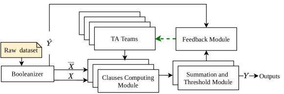
Figure 1: Block diagram of TM (dashed green arrow indicates penalties and rewards)[19]

A fundamental difference between the TM and NNs is the requirement of a Booleanizer module. The key premise is to convert the raw input features and their complements to Boolean features rather than binary encoded features as seen with NNs. These Boolean features are also referred to as literals: $\hat{X}$ and ${X}$. Current research has shown that significance-driven Booleanization of features for the Tsetlin Machine is vital in controlling the Tsetlin Machine size and processing requirements [18]. Increasing the number of features will increase the number of TA and increase computations for the clause module and subsequently the energy spent in incrementing and decrementing states in the feedback module. The choice of the number of clauses to represent the problem is also available as a design knob, which also directly affects energy/accuracy tradeoffs [19].

The Tsetlin Machine also has two hyper parameters, the s value and the Threshold (T). The Threshold parameter is used to determine the clause selection to be used in the voting mechanism, larger Thresholds will mean more clauses partake in the voting and influence the feedback to TA states. The s value is used to control the fluidity with which the TAs can transition between states. Careful manipulation of these parameters can be used to determine the flexibility of the feedback module and therefore control the TMs learning stability [17]. As seen in Figure 2, increasing the Threshold and decreasing the s value will lead to more events triggered as more states are transitioned. These parameters must be carefully tuned to balance energy efficiency through minimizing events triggered, and achieving good performance through finding the optimum s-T range for learning stability in the KWS application.

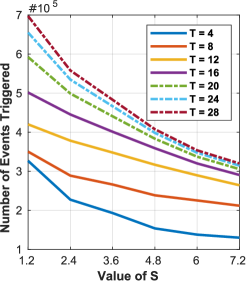
Figure 2: The affect of $T$ and $s$ on reinforcements on TM[19]

In order to optimize the TM for KWS, due diligence must be given to designing steps that minimize the Boolean feature set. This allows for finding a balance between performance and energy usage through varying the TM hyper parameters and the number of clause computation modules. Through exploitation of these relationships and properties of the TM, the KWS pipeline can be designed with particular emphasis on feature extraction and minimization of the number of the TMs clause computation modules. An extensive algorithmic description of Tsetlin Machine can be found in [16]. The following section will detail how these ideas can be implemented through audio pre-processing and Booleanization techniques for KWS.

3 Audio Pre-processing Techniques for KWS

When dealing with audio data, the fundamental design efforts in pre-processing should be to find the correct balance between reducing data volume and preserving data veracity. That is, while removing the redundancies from the audio stream the data quality and completeness should be preserved. This is interpreted in the proposed KWS-TM pipeline through two methods: feature extraction through MFCCs, followed by discretization control through quantile based binning for Booleanization. These methods are expanded below.

3.1 Audio Feature Extraction using MFCC

Audio data streams are always subject to redundancies in the channel that formalize as nonvocal noise, background noise and silence [20, 21]. Therefore the challenge becomes identification and extraction of the desired linguistic content (the keyword) and maximally discarding everything else. To achieve this we must consider transformation and filtering techniques that can amplify the characteristics of the speech signals against the background information. This is often done through the generation of MFCCs as seen in the signal processing flow in Figure 3.

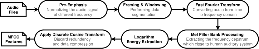
Figure 3: MFCC pipeline.

The MFCC is a widely used audio file pre-processing method for speech related classification applications [22, 21, 23, 24, 25, 12]. The component blocks in the MFCC pipeline are specifically designed for extracting speech data taking into account the intricacies of the human voice.

The Pre-Emphasis step is used to compensate for the structure of the human vocal tract and provide initial noise filtration. When producing glottal sounds when speaking, higher frequencies are damped by the vocal tract which can be characterized as a step roll-off in the signals’ frequency spectrum [26]. The Pre-Emphasis step, as its name-sake suggests, amplifies (adds emphasis to) the energy in the high frequency regions, which leads to an overall normalization of the signal [27].

Speech signals hold a quasi-stationary quality when examined over a very short time period, which is to say that the statistical information it holds remains near constant [20]. This property is exploited through the Framing and Windowing step. The signal is divided into around 20ms frames, then around 10-15ms long window functions are multiplied to these overlapping frames, in doing so we preserve the temporal changes of the signal between frames and minimize discontinuities (this is realized through the smoothed spectral edges and enhanced harmonics of the signal after the subsequent transformation to the frequency domain) [28]. The windowed signals are then transformed to the frequency domain through a Discrete Fourier Transform (DFT) process using the Fast Fourier Transform (FFT) algorithm. FFT is chosen as it is able to find the redundancies in the DFT and reduce the amount of computations required offering quicker run-times.

The human hearing system interprets frequencies linearly up to a certain range (around 1KHz) and logarithmically thereafter. Therefore, adjustments are required to translate the FFT frequencies to this non-linear function [29]. This is done through passing signal through the Mel Filter Banks in order to transform it to the Mel Spectrum [30]. The filter is realized by overlapping band-pass filters to create the required warped axis. Next, the logarithm of the signal is taken, this brings the data values closer and less sensitive to the slight variations in the input signal [30]. Finally we perform a Discrete Cosine Transform (DCT) to take the resultant signal to the Cepstrum domain [31]. The DCT function is used as energies present in the signal are very correlated as a result of the overlapping Mel filterbanks and the smoothness of the human vocal tract; the DCT finds the co-variance of the energies and is used to calculate the MFCC features vector [27, 32]. This vector can be passed to the Booleanizer module to produce the input Boolean features, as described next.

3.2 Feature Booleanization

As described in Section 2, Booleanization is an essential step for logic based feature extraction in Tsetlin Machines. Minimizing the Boolean feature space is crucial to the Tsetlin Machine’s optimization. The size and processing volume of a TM is primarily dictated by the number of Booleans [18]. Therefore, a pre-processing stage for the audio features must be embedded into the pipeline before the TM to allow for granularity control of the raw MFCC data. The number of the Booleanized features should be kept as low as possible while capturing the critical features for classification [18].

The discretization method should be able to adapt to, and preserve the statistical distribution of the MFCC data. The most frequently used method in categorizing data is through binning. This is the process of dividing data into group, individual data-points are then represented by the group they belong to. Data points that are close to each other are put into the same group thereby reducing data granularity  [16]. Fixed width binning methods are not effective in representing skewed distribution and often result in empty bins, they also require manual decision making for bin boundaries.

Therefore, for adaptive and scalable Booleanization quantile based binning is preferred. Through binning the data using its own distribution, we maintain its statistical properties and do not need to provide bin boundaries, merely the number of bins the data should be discretized into. The control over the number of quantiles is an important parameter in obtaining the final Boolean feature set. Choosing two quantiles will result in each MFCC coefficient being represented using only one bit; however, choosing ten quantiles (or bins) will result in four bits per coefficient. Given the large number of coefficients present in the KWS problem, controlling the number of quantiles is an effective way to reduce the total TM size.

3.3 The KWS-TM pipeline

The KWS-TM pipeline is composed of the the data encoding and classification blocks presented in Figure 4. The data encoding scheme encompasses the generation of MFCCs and the quantile binning based Booleanization method. The resulting Booleans are then fed to the Tsetlin Machine for classification. The figure highlights the core attributes of the pre-processing blocks: the ability to extract the audio features only associated with speech through MFCCs and the ability to control their Boolean granularity through quantile binning.

To explore the functionality of the pipeline and the optimizations that can be made, we return to our primary intentions, i.e., to achieve energy efficiency and high learning efficacy in KWS applications. We can now use the design knobs offered in the pre-processing blocks, such as variable window size in the MFCC generation, and control over the number of quantiles to understand how these parameters can be used in presenting the Boolean data to the TM in a way to returns good performance utilizing the least number of Booleans. Through Section 2 we have also seen the design knobs available through variation of the hyperparameters s and Threshold T, as well as the number of clause computation modules used to represent the problem. Varying the parameters in both the encoding and classification stages through an experimental context will uncover the impact they have on the overall KWS performance and energy usage.

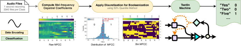
Figure 4: The data encoding and classification stages in the KWS-TM pipeline

4 Experimental Results

To evaluate the proposed KWS-TM pipeline, Tensorflow speech command dataset was used. The dataset consists of many spoken keywords collected from a variety of speakers with different accents, as well as male and female gender. The datapoints are stored as 1 second long audio files where the background noise is negligible. This reduces the effect of added redundancies in the MFCC generation, given our main aim is predominantly to test functionality, we will explore the impact of noisy channels in our future work. This dataset is commonly used in testing the functionality of ML models and will therefore allow for fair comparisons to be drawn [33].

From the Tensorflow dataset, 10 keywords: "Yes", "No", "Stop", "Seven", "Zero", "Nine", "Five", "One", "Go" and "Two", have been chosen to explore the functionality of the pipeline using some basic command words. Considering other works comparing NN based pipelines, 10 keywords is the maximum used [34, 13]. Among the keywords chosen, there is an acoustic similarity between "No" and "Go", therefore, we explore the impact of 9 keywords together (without "Go") and then the effect of "No" and "Go" together. The approximate ratio of training data, testing data and validation data is given as 8:1:1 respectively with a total of 3340 datapoints per class. Using this setup, we will conduct a series of experiments to examine the impact of the various parameters of the KWS-TM pipeline discussed earlier. The experiments are as follows:

• Manipulating the window length and window steps to control the number of MFCCs generated.

• Exploring the effect of different quantile bins to change the number of Boolean features.

• Using a different number of the keywords ranging from the 2 to 9 to explore the scalability of the pipeline.

• Testing the effect on performance of acoustically different and similar keywords.

• Changing the size of the TM through manipulating the number of clause computation modules, optimizing performance through tuning the feedback control parameters s and T.

4.1 MFCC Setup

It is well defined that the number of input features to the TM is one of the major factors that affect its resource usage [17, 18, 19]. Increased raw input features means more Booleans are required to represent them and thus the number of Tsetlin Automaton (TA) in the TM will also increase leading to more energy required to provide feedback to them. Therefore, reducing the number of features at the earliest stage of the data encoding stage of the pipeline is crucial to implementing energy-frugal TM applications.

The first set of parameters available in manipulating the number of features comes in the form of the Window Step and the Window Length (this takes place in the "Framing an Windowing" stage in Figure 4) in MFCC generation and can be seen through Figure 5(a).

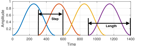
(a) The windowing process.

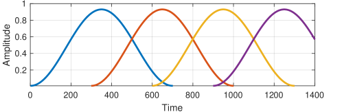
(b) Effect of increasing window length.

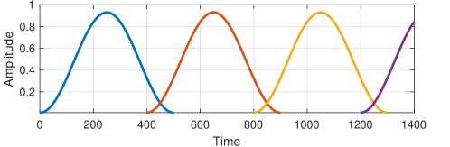
(c) Effect of increasing window step.

Figure 5: The Hamming window function applied to audio pre-processing.

The window function is effective in reducing the spectral distortion by tapering the sample signal at the beginning and ending of each frame (We use overlapping frames to ensure signal continuity is not lost). Smaller Window Steps lead to a more fine grained and descriptive representation of the audio features through more frames and therefore more MFCCs but this also increases computations and latency.

Increasing the Window Length leads to a linear decrease in the total number of frames and therefore the MFCCs as seen in Figure 6(a). Given that the Window Steps are kept constant for this experiment, we have a linearly decreasing number of window overlaps resulting in a linearly decreasing total number of window functions, FFTs and subsequent computations. This leads to the linear decrease in the MFCCs across all frames.

Increasing the Window Step leads to much sharper fall given the overlapping regions now no longer decrease linearly as seen in Figure 6(b). This results in a total number of non-linearly decreasing window functions and therefore much fewer FFTs and so on, leading to much fewer MFCCs across all frames. As a result of this, the smaller the increase in the Window Step the larger the decrease in the number of frames and therefore MFCCs.

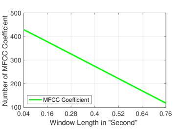
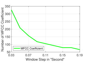
(a) The effect of increasing window length.	(b) The effect of increasing window step.

Figure 6: Changing the number of MFCC coefficients through manipulating the Window parameters.

To test the effectiveness of manipulating the Window Length and Window Step, the MFCC coefficients were produced for 4 keywords and the TMs classification performance was examined as seen in Figure 7(a) and Figure 7(b). Changing the Window Length results in much bigger falls in accuracy compared to Window Step. This is due to the diminished signal amplitudes at the window edges, longer windows mean more tapering of the edge amplitudes and fewer overlaps to preserve the signal continuities as seen through Figure 5(b). As a result, the fidelity of generated the MFCC features is reduced.

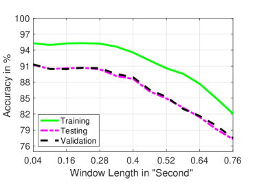
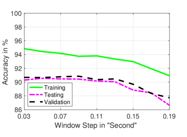
(a) Effect of window length on accuracy.	(b) Effect of window step on accuracy.

Figure 7: Effect of changing window parameters on classification accuracy.

The effect of increasing the Window Step leads to a smaller drop in accuracy. We see the testing and validation accuracy remain roughly the same at around 90.5$\%$ between 0.03 and 0.10 second Window Steps and then experience a slight drop. Once again this is due to the tapering effect of the window function, given the window length remains the same for this experiment, we know that the increasing of window steps will mean far fewer total overlaps and a shrinking overlapping region as seen in Figure 5(c). The overlaps are used to preserve the continuity of the signal against the window function edge tapering, as the size of the overlapping regions decrease, the effect of edge tapering increases thereby leading to increased loss of information. The accuracy remains constant up to a Window Step of 0.1s as the Window Length is sufficiently long to capture enough of the signal information, once the overlapping regions start to shrink we experience the loss in accuracy.

We can see that increasing the Window Step is very effective in reducing the number of frames and therefore the total number MFCC coefficients across all frames and providing the Window Length is long enough, the reduction in performance is minimal. To translate these findings toward energy efficient implementations, we must give increased design focus to finding the right balance between the size of the Window Step parameter and the achieved accuracy given the reduction in computations from the reduction in features produced.

4.2 Impact of Number of Quantiles

Increased granularity through more bins will lead to improved performance but it is observed that this is not the case entirely. Table 1 shows the impact of the KWS-TM performance when increasing the number of bins. The testing and validation accuracy remain around the same with 1 Boolean per feature compared with 4 Booleans per feature. Figure 8 shows the large variance in some feature columns and no variance in others. The zero variance features are redundant in the subsequent Booleanization, they will be represented through the same Boolean sequence. The features with large variances are of main interest. We see that the mean for these features is relatively close to zero compared to their variance (as seen in Figure 9), therefore one Boolean per feature representation is sufficient, a 1 will represent values above the mean and 0 will represent below. The logical conclusion to be made from these explorations is that the MFCC alone is sufficient in both eliminating redundancies and extracting the keyword properties and does not require additional granularity beyond one Boolean per feature to distinguish classes.

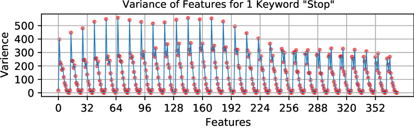
Figure 8: Variance between MFCC features.

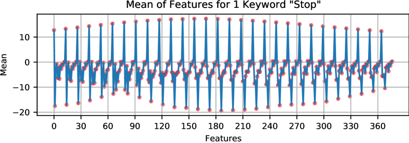
Figure 9: Mean of MFCC features.

We have seen that the large variance of the MFCCs mean that they are easily represented by 1 Boolean per feature and that is sufficient to achieve high performance. This is an important initial result, for offline learning we can now also evaluate the effect of removing the no variance features in future work to further reduce the total number of Booleans. From the perspective of the Tsetlin Machine there is an additional explanation as to why the performance remains high even when additional Boolean granularity is allocated to the MFCC features. Given that there are a large number datapoints in each class (3340), if the MFCCs that describe these datapoints are very similar then the TM will have more than sufficient training data to settle on the best propositional logic descriptors. This is further seen by the high training accuracy compared to the testing and validation accuracy.

Table 1: Impact of increasing quantiles with 4 classes

Training	Testing	Validation	Num.Bins	Bools per Feature	Total Bools
94.8%	91.3%	91.0%	2	1	378
96.0%	92.0%	90.7%	4	2	758
95.9%	90.5%	91.0%	6	3	1132
95.6%	91.8%	92.0%	8	3	1132
97.1%	91.0%	90.8%	10	4	1512

4.3 Impact of Increasing the Number of Keywords

Figure 10(a) shows the linear nature with which the training, testing and validation accuracy decrease as the number of keywords are increased for a TM with 450 clauses with 200 epochs for training. We note that the testing and validation accuracy start to veer further away from the training accuracy with the increase of keywords. This performance drop is expected in ML methods as the problem scales [35]. Despite the large number of datapoints per keyword this is an indicator of overfitting, as confirmed through Figure 10(b) showing around a 4$\%$ increase. The implication of this is that increased number of keywords make it difficult for the TM to create distinct enough propositional logic to separate the classes. The performance drop is caused when the correlation of keywords outweighs the number of datapoints to distinguish each of them. This behavior is commonly observed in ML models for audio classification applications [23].

The explained variance ratio of the dataset with an increasing number of keywords was taken for the first 100 Principle Component Analysis eigenvalues, as seen in Figure 10(b). We observe that as the number of keywords is increased, the system variance decreases, i.e. the inter-class features start to become increasingly correlated. Correlated inter-class features will lead to class overlap and degrade TM performance [18]. Through examination of the two largest Linear Discriminant component values for the 9 keyword dataset, we clearly see in Figure 11 that there is very little class separability present.

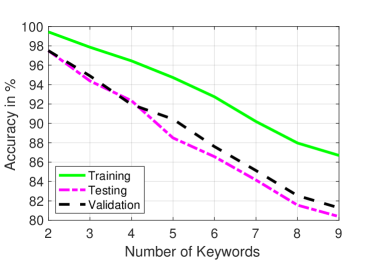
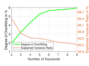
(a) The effect on accuracy.	(b) The amount of overfitting.

Figure 10: The effect of increasing the number of keywords.

To mitigate against the effect on performance of increasing keywords, there are two methods available: Firstly to adjust the Tsetlin Machines hyperparameters to enable more events triggered (see Figure 2). In doing so the this may allow the TM to create more differing logic to describe the classes. Then, by increasing the number of clause computation modules, the TM will have a larger voting group in the Summation and Threshold module and potential reach the correct classification more often. Secondly the quantity of the datapoints can be increased, however, for this to be effective the new dataset should hold more variance and completeness when describing each class. This method of data regularization is often used in audio ML applications to deliberately introduce small variance between datapoints [21].

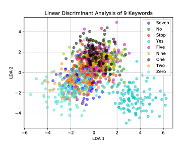
Figure 11: LDA of 9 keywords.

4.4 Acoustically Similar Keywords

In order to test the robustness of the KWS-TM pipeline functionality, we must emulate real-word conditions where a user will use commands that are acoustically similar to others. Table 2 shows the results of such circumstances. The Baseline experiment is a KWS dataset consisting of 3 keywords: ’Yes’, ’No’ and ’Stop’. The second experiment then introduces the keyword ’Seven’ to the dataset and the third experiment introduces the keyword ’Go’.

The addition of ’Seven’ causes a slight drop in accuracy adhering to our previously made arguments of increased correlation and the presence of overfitting. However the key result is the inclusion of ’Go’; ’Go’ is acoustically similar to ’No’ and this increases the difficulty in separating these two classes. We see from Figure 12(a), showing the first two LDA components that adding ’Seven’ does not lead to as much class overlap as adding ’Go’ as seen in Figure 12(b). As expected, the acoustic similarities of ’No’ and ’Go’ lead to significant overlap. We have seen from the previous result (Figure 11) that distinguishing class separability is increasingly difficult when class overlaps are present.

Table 2: Impact of acoustically similar keywords.

Experiments	Training	Testing	Validation
Baseline	94.7%	92.6%	93.1%
Baseline + ‘Seven’	92.5%	90.1%	90.2%
Baseline + ‘Go’	85.6%	82.6%	80.9%

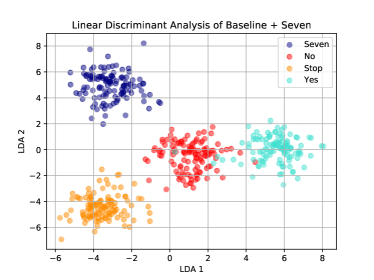
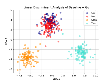
(a) The Baseline with ‘Seven’.	(b) The Baseline with ‘Go’.

Figure 12: The LDA of 4 keywords - the Baseline with one other.

4.5 Number of Clauses per Class

So far we have considered the impact of Booleanization granularity, problem scalabilty and robustness when dealing with acoustically similar classes. Now, we turn our attention towards optimizing the KWS-TM pipeline to find the right functional balance between performance and energy efficiency. This is made possible through two streams of experimentation: manipulating the number of clauses for each keyword class in the TM and observing the energy expenditure and accuracy, and experimenting with the TMs hyperparameters to enable better performance using fewer clauses.

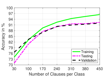
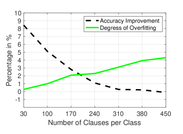
(a) The effect on accuracy.	(b) The effect on overfitting.

Figure 13: Effect of increasing the number of clauses on accuracy and overfitting.

The influence of increasing the number of clauses was briefly discussed in Section 2, here we can see the experimental result in Figure 13(a) showing the impact of increasing clauses with 4 classes.

Increased number of clauses leads to better performance. However, upon closer examination we can also see the impact of overfitting at the clause level, i.e., increasing the number of clauses has resulted in a larger difference in the training accuracy with the testing and validation. The datapoints for the 4 classes were sufficient to create largely different sub-patterns for the TAs during training, but not complete enough to describe new data in the testing and validation.

As a result, when clauses are increased, more clauses reach incorrect decisions and sway the voting in the summation and threshold module toward incorrect classification, which is seen through Figure 14(a). The TM has two types of feedback, Type I, which introduces stochasticity to the system and Type II, which bases state transitions on the results of corresponding clause value. Type II feedback is predominantly used to diminish the effect of false positives. We see that as the clause value increases the TM uses more Type II feedback indicating increased false positive classifications. This result is for due to the incompleteness in the training data in describing all possible logic propositions for each class. We see this through 14(b); despite increasing the number of epochs we do not experience a boost in testing and validation accuracy and through Figure 13(b) we find the point where the overfitting outweighs the accuracy improvement at around 190-200 clauses.

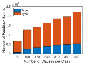
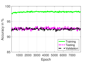
(a) The effect of clauses on feedback.	(b) The effect of epoch on accuracy.

Figure 14: Effect of increasing the number of clauses on TM feedback (a), and the effect of increasing the number of epochs on accuracy (b).

From the perspective of energy efficiency, these results offer two possible implications for the KWS-TM pipeline, if a small degradation of performance in the KWS application is acceptable, then operating at a lower clause range will be more beneficial for the TM. The performance can then be boosted through hyperparameters available to adjust feedback fluidity. This approach will reduce energy expenditure through fewer clause computations and reduce the effects of overfitting when the training data lacks enough completeness. Alternatively, if performance is the main goal, then the design focus should be on injecting training data with more diverse datapoints to increase the descriptiveness of each class. In that case, increased clauses will provide more robust functionality.

Table 3: Impact of the number of clauses on energy/accuracy tradeoffs.

	Clauses	Current	Time	Energy	Accuracy
Training	100	0.50 A	68 s	426.40 J	-
Training	240	0.53 A	96 s	636.97 J	-
Inference	100	0.43 A	12 s	25.57 J	80 %
Inference	240	0.47 A	37 s	87.23 J	90 %

The impacts of being resource efficient and energy frugal are most prevalent when implementing KWS applications into dedicated hardware and embedded systems. To explore this practically, the KWS-TM pipeline was implemented onto a Raspberry Pi. The same 4 keyword experiement was ran with 100 and 240 clauses. As expected, we see that increased clause computations lead to increased current, time and energy usage, but also delivers better performance. We can potentially boost the performance of the Tsetlin Machine at lower clauses through manipulating the hyperparameters as seen Table 4.

Table 4: Impact of the T values on accuracy

Clauses	T	Training	Testing	Validation	Better Classification
30	2	83.5 %	80.5 %	83.8 %	✓
30	23	74.9 %	71.1 %	76.1 %
450	2	89.7 %	86.1 %	84.9 %
450	23	96.8 %	92.5 %	92.7 %	✓

The major factor that has impacted the performance of the KWS is the capacity of the TM which is determined by the number of clauses per class. The higher the number clauses, the higher the overall classification accuracy [18]. Yet, the resource usage will increase linearly along with the energy consumption and memory footprint. Through Table 4 we see that at 30 clauses the accuracy can be boosted through reducing the Threshold hyperparameter. The table offers two design scenarios; firstly, very high accuracy is achievable through a large number of clauses (450 in this case) and a large Threshold value. With a large number of clauses an increased number of events must be triggered in terms of state transitions (see Figure 2) to encourage more feedback to clauses and increases the TMs decisiveness. While this offers a very good return on performance, the amount of computations are increased with more clauses and more events triggered and this leads to increased energy expenditure as seen through Table 3.

In contrast, using 960 clauses and a lower Threshold still yields good accuracy but at a much lower energy expenditure through fewer clause computations and feedback events. A smaller number of clauses mean that the vote of each clause has more impact, even at a smaller Threshold the inbuilt stochasticity of the TM’s feedback module allows the TAs to reach the correct propositional logic. Through these attributes it is possible to create more energy frugal TMs requiring fewer computations and operating at a much lower latency.

4.6 Comparative Learning Convergence and Complexity Analysis of KWS-TM

Both TMs and NNs have modular design components in their architecture; For the TM, this is in the form of clauses and for the NN it is the number of neurons. NNs require input weights for the learning mechanism which define the neurons’ output patterns. The number of weights and the number of neurons are variable, however more neurons will lead to better overall NN connectivity due to more refined arithmetic pathways to define a learning problem.

For the TM the clauses are composed of TAs. The number of TAs are defined by the number of Boolean features which remains static throughout the course of the TMs learning. It is the number of clauses that is variable, increasing the clauses typically offers more propositional diversity to define a learning problem.

Through Figure 15 and Table 5 we investigate the learning convergence rates of the TM against 4 ’vanilla’ NN implementations. The TM is able to converge to 90.5$\%$ after less than 10 epochs highlighting its quick learning rate compared to NNs which require around 100 epochs to converge to the isoaccuracy target ($\approx$90%). After further 100 epochs the NN implementations reach only marginally better accuracy than TM. The indirect implication of faster convergence is improved energy efficiency as fewer training epochs will result in fewer computations required for the TA states to settle.

Table 5 shows one of the key advantages of the TM over all types of NNs, the significantly fewer parameters required, i.e. low-complexity. Large number of parameters needed for NNs are known to limit their practicality for on-chip KWS solutions [34, 36, 12, 13], where as the TM offers a more resource-frugal alternative. With only 960 clauses, which require only logic based processing, the TM outperforms even the most capable large and deep NNs. In our future work, we aim to exploit this to enable on-chip learning based KWS solutions.

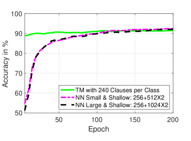
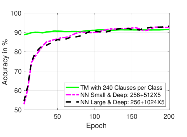
(a) Convergence of the TM against shallow NNs.	(b) Convergence of the TM against deep NNs.

Figure 15: Training convergence of TM and NN implementations.

Table 5: The required parameters for different NNs and the TM for a 4 keyword problem.

KWS-ML Configuration	Num. neurons	Num. hyperparameters
NN Small & Shallow: 256+512X2	1,280	983,552
NN Small & Deep: 256+512X5	2,816	2,029,064
NN Large & Shallow: 256+1024X2	2,304	2,822,656
NN Large & Deep: 256+1024X5	5,376	7,010,824
TM with 240 Clauses per Class	960 (clauses)	2 hyperparameters with 725760 TAs

5 Related Work

This section will provide a brief examination into current KWS research, industrial challenges with KWS, deeper look in the component blocks of the TM and provide insight into the current developments and the future research directions.

5.1 Current KWS developments

The first KWS classification methods proposed in the late 1970s used MFCCs for their feature extraction ability and because the coefficients produced offered a very small dimensionality compared to the raw input data that was being considered then [37]. It was later shown that compared to other audio extraction methods such as near prediction coding coefficients (LPCC)s and perceptual linear production (PLP), MFCCs perform much better with increased background noise and low SNR [12].

For the classifier, Hidden Markov Models (HMMs) were favored after the MFCC stage due to their effectiveness in modelling sequences [37]. However they rely on many summation and Bayesian probability based arithmetic operations as well as the computationally intensive Viterbi decoding to identify the final keyword [34, 38, 39].

Later it was shown that Recurrent Neural Networks (RNN)s outperform HMMs but suffer from operational latency as the problem scales, albeit RNNs still have faster run-times than HMM pipelines given they do not require a decoder algorithm [38]. To solve the latency issue, the Deep Neural Network (DNN) was used, it has smaller memory footprint and reduced run-times compared to HMMs [12, 39]. However, DNNs are unable to efficiently model the temporal correlations of the MFCCs and their transitional variance [36] [34]. In addition to this, commonly used optimization techniques used for DNNs such as pruning, encoding and quantization lead to great accuracy losses with KWS applications [12].

The MFCC features exist as a 2D array as seen in Figure 4, to preserve the temporal correlations and transitional variance, this array can be treated as an image and a convolutional neural network (CNN) can be used for classification [13, 36]. With the use of convolution comes the preservation of the spatial and temporal dependencies of the 2D data as well as the reduction of features and computations from the convolution and pooling stages [13]. However, once again both the CNN and DNN suffer from the large number of parameters (250K for the dataset used in [36] and 9 million Multiplies required for the CNN). Despite the gains in performance and reductions in latency, the computational complexity and large memory requirements from parameter storage are ever present with all NN based KWS solutions.

The storage and memory requirements played a major part in transitioning to a micro-controller system for inference where memory is limited through the size of the SRAM [34]. In order to accommodate for the large throughput of running NN workloads, micro-controllers with integrated DSP instructions or integrated SIMD and MAC instructions can accelerate low-precision computations [34]. When testing for 10 keywords, it was shown experimentally in [34], that for systems with limited memory and compute abilities DNNs are favorable given they use the fewer operations despite having a lower accuracy (around 6$\%$ less) compared to CNNs.

It is when transitioning to hardware that the limitations of memory and compute resources become more apparent. In these cases it is better to settle for energy efficiency through classifiers with lower memory requirements and operations per second even if there is a slight drop in performance.

A 22nm CMOS based Quantized Convolutional Neural Network (QCNN) Always-ON KWS accelerator is implemented in [12], they explore the practicalities of CNN in hardware through quantized weights, activation values and approximate compute units. Their findings illustrate the effectiveness of hardware design techniques; the use of approximate compute units led to a significant decrease in energy expenditure, the hardware unit is able to classify 10 real-time keywords under different SNRs with a power consumption of 52$\mu$W. This impact of approximate computing is also argued in [13] with design focus given to adder design, they propose an adder with a critical path that is 49.28$\%$ shorter than standard 16-bit Ripple Carry Adders.

Through their research work with earables Nokia Bell Labs Cambridge have brought an industrial perspective to the idea of functionality while maintaining energy frugality into design focus for AI powered KWS [40, 41], with particular emphasis on user oriented ergonomics and commercial form factor. They discovered that earable devices are not as influenced by background noise compared to smartphones and smartwatches and offer better signal-to-noise ratio for moving artefacts due to their largely fixed wearing position in daily activities (e.g. walking or descending stairs) [41]. This was confirmed when testing using Random Forest classifiers.

5.2 The Tsetlin Machine

We briefly discussed the overall mechanism of the TM and the main building blocks in the Section 2. In this section, we will have a closer look to the fundamental learning element of the TM, namely the Tsetlin Automaton, as described in Figure 16. We will also present a more detailed look at the clause computing module as seen in Figure 17, and we will discuss the first application-specific integrated circuit (ASIC) implementation of the TM, the Mignon , as seen in Figure 18.

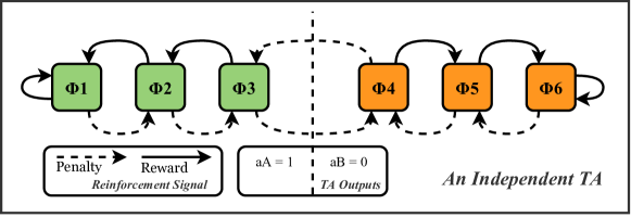
Figure 16: Mechanism of a TA.

The TA is the most fundamental part of the TM forming the core learning element that drives classification (Figure 16). Developed by Mikhail Tsetlin in the 1950s, the TA is an FSM where the current state will transition towards or away from the middle state upon receiving Reward or Penalty reinforcements during the TMs training stage. The current state of the TA will decide the output of the automaton which will be either an Include (aA) or Exclude (aB).

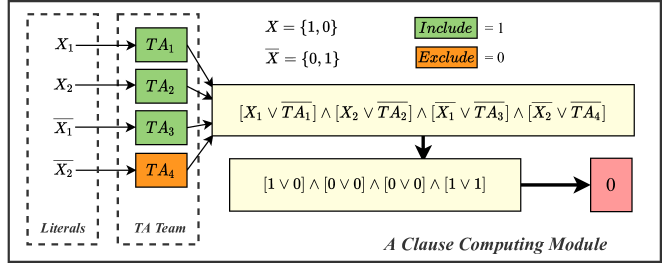
Figure 17: Mechanism of a Clause computing module (assuming TA₁= 1 means Include and TA₁= 0 means Exclude).

Figure 17 shows how the clause module create logic propositions that describe the literals based on the TA decisions through logic OR operations between the negated TA decision and the literal. The TA decision is used to bit mask the literal and through this we can determine which literals are to be excluded. The proposition is then logic ANDed and this forms the raw vote for this clause. Clauses can be of positive and negative polarity, as such, a sign will be added to the clause output before it partakes in the class voting. It is important to note the reliance purely on logic operations making the TM well suited to hardware implementations. Clauses are largely independent of each other, only coalescing for voting giving the TM good scalability potential.

The feedback to the TM can be thought of on three levels, at the TM level, at the clause level and at the TA level. At the TM level, the type of feedback to issue is decided based on the target class and whether the TM is in learning or inference mode. For inference no feedback is given, we simply take the clause computes for each class and pass to the summation and threshold module to generate the predicted class. However, in training mode there is a choice of Type I feedback to combat false negatives or Type II feedback to combat false positives. This feedback choice is further considered at the clause level.

At the clause level there are three main factors that will determine feedback type to the TAs, the feedback type decision from the TM level, the current clause value, and whether the magnitude of clause vote is above the magnitude of the Threshold.

At the TA level, the feedback type from the clause level will be used in conjunction with the current TA state and the s parameter to determine whether there is inaction, penalty or reward given to the TA states.

The simplicity of the TM shows its potential to be a promising NN alternative. Lei et al [19] comparatively analyzed the architecture, memory footprint and convergence of these two algorithms for different datasets. This research shows the fewer number of hyperparameter of the TM will reduce the complexity of the design. The convergence of the TM is higher than the NN in all experiments conducted.

The most unique architectural advances of the TM is the propositional logic based learning mechanism which will be beneficial in achieving energy frugal hardware AI. Wheeldon et al. [18] presented the first ASIC implementation of the TM for Iris flower classifications (see Figure 18).

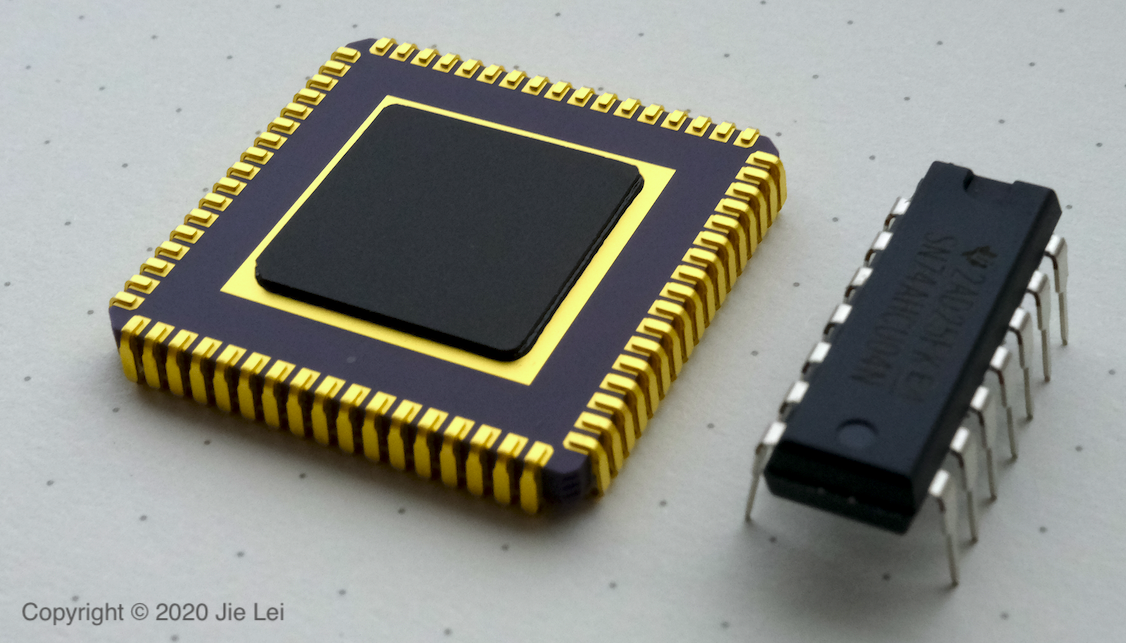
Figure 18: The Mignon AI: ASIC microchip acclerating TM (left).

This 65-nm technology based design is a breakthrough in achieving an energy efficiency of up to 63 Tera Operations per Joule (Tops/Joule) while maintaining high convergence rate and performance. The early results from this microchip has been extensively compared with Binarized Convolutional Neural Network (BCNN) and neuromorphic designs in [18].

In addition, Wheeldon et al. [18] also proposed a system-wide design space exploration pipeline in deploying TM into ASIC design. They introduced a detailed methodology from 1) dataset encoding building on the work seen in [4] to 2) software based design exploration and 3) an FPGA based hyperparameter search to 4) final ASIC synthesis. A follow-up work of this [42] also implemented a self-timed and event-driven hardware TM. This implementation showed power and timing elasticity properties suitable for low-end AI implementations at-the-microedge.

Other works include mathematical lemma based analysis of clause convergence using the XOR dataset [43], natural language (text) processing [44], disease control [4], methods of automating the s parameter [45] as well as exploration of regression and convolutional TMs [46, 47].

The TM has so far, been implemented with many different programming languages such as, C, C++, C$\#$, Python and Node.js, to name a few. It has also been optimized for High Performance Computing (HPC) through Compute Unified Device Architecture (CUDA) for accelerating Graphics Processing Unit (GPU) based solutions and currently through OpenCL for heterogeneous embedded systems [48].

Exploiting the natural logic underpinning there are currently ongoing efforts in establishing explainability evaluation and analysis of TMs[17]. Deterministic implementation of clause selection in TM, reported by [49], is a promising direction to this end.

Besides published works, there are numerous talks, tutorials and multimedia resources currently available online to mobilize the hardware/software community around this emerging AI algorithm. Below are some key sources:

Videos: https://tinyurl.com/TMVIDEOSCAIR.

Publications: https://tinyurl.com/TMPAPERCAIR & www.async.org.uk.

Software implementations: https://tinyurl.com/TMSWCAIR

Hardware implementations, Mignon AI: http://www.mignon.ai/.

A short video demonstrating KWS using TM can be found here:
https://tinyurl.com/KWSTMDEMO.

6 Summary and Conclusions

The paper presented the first ever TM based KWS application. Through experimenting with the hyperparameters of the proposed KWS-TM pipeline we established relationships between the different component blocks that can be exploited to bring about increased energy efficiency while maintaining high learning efficacy.

From current research work we have already determined the best methods to optimize for the TM is through finding the right balance between reduction of the number of features, number of clauses and number of events triggered through the feedback hyper-parameters against the resulting performance from these changes. These insights were carried into our pipeline design exploration experiments.

Firstly, we fine tuned the window function in the generation of MFCCs, we saw that increasing the window steps lead to much fewer MFCCs and if the window length is sufficient enough to reduce edge tapering then the performance degradation is minimal. Through quantile binning to manipulate the discretization of the Boolean MFCCs, it was seen that this did not yield change in performance. The MFCC features of interest have very large variances in each feature column and as such less precision can be afforded to them, even as low as one Boolean per feature. This was extremely useful in reducing the resulting TM size.

Through manipulating the number of clause units to the TM on a Raspberry Pi, we confirmed the energy and latency savings possible by running the pipeline at a lower clause number and using the Threshold hyper-parameter the classification of the accuracy can also be boosted. Through these design considerations we are able to increase the energy frugality of the whole system and transition toward low-power hardware accelerators of the pipeline to tackle real time applications.

The KWS-TM pipeline was then compared against some different NN implementations, we demonstrated the much faster convergence to the same accuracy during training. Through these comparisons we also highlighted the far fewer parameters required for the TM as well as a fewer number of clauses compared to neurons. The faster convergence, fewer parameters and logic over arithmetic processing makes the KWS-TM pipeline more energy efficient and enables future work into hardware accelerators to enable better performance and low power on-chip KWS.

Acknowledgement: The authors gratefully acknowledge the funding from EPSRC IAA project “Whisperable” and EPSRC grant STRATA (EP/N023641/1). The research also received help from the computational powerhouse at CAIR.

7 Future Work

Through testing the KWS-TM pipeline against the Tensorflow Speech data set we did not account for background noise effects. In-field IoT applications must be robust enough to minimize the effects of additional noise, therefore, future work in this direction should examine the effects of the pipeline with changing signal-to-noise ratios. The pipeline will also be deployed to a micro-controller in order to benefit from the effects of energy frugality by operating at a lower power level.

References

- [1] T. Rausch and S. Dustdar. Edge intelligence: The convergence of humans, things, and ai. In 2019 IEEE International Conference on Cloud Engineering (IC2E), pages 86–96, 2019.
- [2] Itsuki Osawa, Tadahiro Goto, Yuji Yamamoto, and Yusuke Tsugawa. Machine-learning-based prediction models for high-need high-cost patients using nationwide clinical and claims data.
- [3] Tiago M. Fernández-Caramés and Paula Fraga-Lamas. Towards the internet-of-smart-clothing: A review on iot wearables and garments for creating intelligent connected e-textiles. Electronics (Switzerland), 7, 12 2018.
- [4] K. D. Abeyrathna, O. C. Granmo, X. Zhang, and M. Goodwin. Adaptive continuous feature binarization for tsetlin machines applied to forecasting dengue incidences in the philippines. In 2020 IEEE Symposium Series on Computational Intelligence (SSCI), pages 2084–2092, 2020.
- [5] K. Hirata, T. Kato, and R. Oshima. Classification of environmental sounds using convolutional neural network with bispectral analysis. In 2019 International Symposium on Intelligent Signal Processing and Communication Systems (ISPACS), pages 1–2, 2019.
- [6] Hadas Benisty, Itamar Katz, Koby Crammer, and David Malah. Discriminative keyword spotting for limited-data applications. Speech Communication, 99:1 – 11, 2018.
- [7] J. S. P. Giraldo, C. O’Connor, and M. Verhelst. Efficient keyword spotting through hardware-aware conditional execution of deep neural networks. In 2019 IEEE/ACS 16th International Conference on Computer Systems and Applications (AICCSA), pages 1–8, 2019.
- [8] J. S. P. Giraldo, S. Lauwereins, K. Badami, H. Van Hamme, and M. Verhelst. 18uw soc for near-microphone keyword spotting and speaker verification. In 2019 Symposium on VLSI Circuits, pages C52–C53, 2019.
- [9] S. Leem, I. Yoo, and D. Yook. Multitask learning of deep neural network-based keyword spotting for iot devices. IEEE Transactions on Consumer Electronics, 65(2):188–194, 2019.
- [10] A depthwise separable convolutional neural network for keyword spotting on an embedded system. EURASIP Journal on Audio, 2020:10, 2020.
- [11] Massimo Merenda, Carlo Porcaro, and Demetrio Iero. Edge machine learning for ai-enabled iot devices: A review. Sensors (Switzerland), 20, 5 2020.
- [12] B. Liu, Z. Wang, W. Zhu, Y. Sun, Z. Shen, L. Huang, Y. Li, Y. Gong, and W. Ge. An ultra-low power always-on keyword spotting accelerator using quantized convolutional neural network and voltage-domain analog switching network-based approximate computing. IEEE Access, 7:186456–186469, 2019.
- [13] S. Yin, P. Ouyang, S. Zheng, D. Song, X. Li, L. Liu, and S. Wei. A 141 uw, 2.46 pj/neuron binarized convolutional neural network based self-learning speech recognition processor in 28nm cmos. In 2018 IEEE Symposium on VLSI Circuits, pages 139–140, 2018.
- [14] Nebojsa Bacanin, Timea Bezdan, Eva Tuba, Ivana Strumberger, and Milan Tuba. Optimizing convolutional neural network hyperparameters by enhanced swarm intelligence metaheuristics. 2020.
- [15] Rishad Shafik, Alex Yakovlev, and Shidhartha Das. Real-power computing. IEEE Transactions on Computers, 2018.
- [16] Ole-Christoffer Granmo. The Tsetlin Machine - A Game Theoretic Bandit Driven Approach to Optimal Pattern Recognition with Propositional Logic. arXiv, April 2018.
- [17] Rishad Shafik, Adrian Wheeldon, and Alex Yakovlev. Explainability and dependability analysis of learning automata based AI hardware. In IEEE IOLTS, 2020.
- [18] Adrian Wheeldon, Rishad Shafik, Tousif Rahman, Jie Lei, Alex Yakovlev, and Ole-Christoffer Granmo. Learning automata based AI hardware design for IoT. Philosophical Trans. A of the Royal Society, 2020.
- [19] J. Lei, A. Wheeldon, R. Shafik, A. Yakovlev, and O. C. Granmo. From arithmetic to logic based ai: A comparative analysis of neural networks and tsetlin machine. In 2020 27th IEEE International Conference on Electronics, Circuits and Systems (ICECS), pages 1–4, 2020.
- [20] S. Chu, S. Narayanan, and C. . J. Kuo. Environmental sound recognition with time–frequency audio features. IEEE Transactions on Audio, Speech, and Language Processing, 17(6):1142–1158, 2009.
- [21] Zohaib Mushtaq and Shun-Feng Su. Environmental sound classification using a regularized deep convolutional neural network with data augmentation. Applied Acoustics, 167:107389, 2020.
- [22] W. Shan, M. Yang, J. Xu, Y. Lu, S. Zhang, T. Wang, J. Yang, L. Shi, and M. Seok. 14.1 a 510nw 0.41v low-memory low-computation keyword-spotting chip using serial fft-based mfcc and binarized depthwise separable convolutional neural network in 28nm cmos. In 2020 IEEE International Solid- State Circuits Conference - (ISSCC), pages 230–232, 2020.
- [23] Muqing Deng, Tingting Meng, Jiuwen Cao, Shimin Wang, Jing Zhang, and Huijie Fan. Heart sound classification based on improved mfcc features and convolutional recurrent neural networks. Neural Networks, 130:22 – 32, 2020.
- [24] L. Xiang, S. Lu, X. Wang, H. Liu, W. Pang, and H. Yu. Implementation of lstm accelerator for speech keywords recognition. In 2019 IEEE 4th International Conference on Integrated Circuits and Microsystems (ICICM), pages 195–198, 2019.
- [25] Kirandeep Kaur and N. Jain. Feature extraction and classification for automatic speaker recognition system – a review. 2015.
- [26] Joseph W. Picone. Signal modeling techniques in speech recognition. In PROCEEDINGS OF THE IEEE, pages 1215–1247, 1993.
- [27] Uday Kamath, John Liu, and James Whitaker. Automatic Speech Recognition, pages 369–404. Springer International Publishing, Cham, 2019.
- [28] Automatic speech recognition. In Speech and Audio Signal Processing, pages 299–300. John Wiley & Sons, Inc., oct 2011.
- [29] N.J. Nalini and S. Palanivel. Music emotion recognition: The combined evidence of mfcc and residual phase. Egyptian Informatics Journal, 17(1):1 – 10, 2016.
- [30] Q. Li, Y. Yang, T. Lan, H. Zhu, Q. Wei, F. Qiao, X. Liu, and H. Yang. Msp-mfcc: Energy-efficient mfcc feature extraction method with mixed-signal processing architecture for wearable speech recognition applications. IEEE Access, 8:48720–48730, 2020.
- [31] C. Paseddula and S. V. Gangashetty. Dnn based acoustic scene classification using score fusion of mfcc and inverse mfcc. In 2018 IEEE 13th International Conference on Industrial and Information Systems (ICIIS), pages 18–21, 2018.
- [32] S. Jothilakshmi, V. Ramalingam, and S. Palanivel. Unsupervised speaker segmentation with residual phase and mfcc features. Expert Systems with Applications, 36(6):9799 – 9804, 2009.
- [33] Pete Warden. Speech commands: A dataset for limited-vocabulary speech recognition, 2018.
- [34] Yundong Zhang, Naveen Suda, Liangzhen Lai, and Vikas Chandra. Hello edge: Keyword spotting on microcontrollers. CoRR, abs/1711.07128, 2017.
- [35] Z. Zhang, S. Xu, S. Zhang, T. Qiao, and S. Cao. Learning attentive representations for environmental sound classification. IEEE Access, 7:130327–130339, 2019.
- [36] Tara Sainath and Carolina Parada. Convolutional neural networks for small-footprint keyword spotting. In Interspeech, 2015.
- [37] J. G. Wilpon, L. R. Rabiner, C. . Lee, and E. R. Goldman. Automatic recognition of keywords in unconstrained speech using hidden markov models. IEEE Transactions on Acoustics, Speech, and Signal Processing, 38(11):1870–1878, 1990.
- [38] Santiago Fernández, Alex Graves, and Jürgen Schmidhuber. An application of recurrent neural networks to discriminative keyword spotting. In Proceedings of the 17th International Conference on Artificial Neural Networks, ICANN’07, page 220–229, Berlin, Heidelberg, 2007. Springer-Verlag.
- [39] G. Chen, C. Parada, and G. Heigold. Small-footprint keyword spotting using deep neural networks. In 2014 IEEE International Conference on Acoustics, Speech and Signal Processing (ICASSP), pages 4087–4091, 2014.
- [40] Chulhong Min, Akhil Mathur, and Fahim Kawsar. Exploring audio and kinetic sensing on earable devices. In Proceedings of the 4th ACM Workshop on Wearable Systems and Applications, WearSys ’18, page 5–10, New York, NY, USA, 2018. Association for Computing Machinery.
- [41] F. Kawsar, C. Min, A. Mathur, and A. Montanari. Earables for personal-scale behavior analytics. IEEE Pervasive Computing, 17(3):83–89, 2018.
- [42] Adrian Wheeldon, Alex Yakovlev, Rishad Shafik, and Jordan Morris. Low-latency asynchronous logic design for inference at the edge. arXiv preprint arXiv:2012.03402, 2020.
- [43] Lei Jiao, Xuan Zhang, Ole-Christoffer Granmo, and K. Darshana Abeyrathna. On the convergence of tsetlin machines for the xor operator, 2021.
- [44] Bimal Bhattarai, Ole-Christoffer Granmo, and Lei Jiao. Measuring the novelty of natural language text using the conjunctive clauses of a tsetlin machine text classifier, 2020.
- [45] Saeed Rahimi Gorji, Ole-Christoffer Granmo, Adrian Phoulady, and Morten Goodwin. A tsetlin machine with multigranular clauses, 2019.
- [46] K Darshana Abeyrathna, Ole-Christoffer Granmo, Xuan Zhang, Lei Jiao, and Morten Goodwin. The regression tsetlin machine: a novel approach to interpretable nonlinear regression. Philosophical Trans. A of the Royal Society, 2019.
- [47] Ole-Christoffer Granmo, Sondre Glimsdal, Lei Jiao, Morten Goodwin, Christian W. Omlin, and Geir Thore Berge. The convolutional tsetlin machine. CoRR, abs/1905.09688, 2019.
- [48] K Darshana Abeyrathna, Bimal Bhattarai, Morten Goodwin, Saeed Gorji, Ole-Christoffer Granmo, Lei Jiao, Rupsa Saha, and Rohan K Yadav. Massively parallel and asynchronous tsetlin machine architecture supporting almost constant-time scaling. arXiv preprint arXiv:2009.04861, 2020.
- [49] K Darshana Abeyrathna, Ole-Christoffer Granmo, Rishad Shafik, Alex Yakovlev, Adrian Wheeldon, Jie Lei, and Morten Goodwin. A novel multi-step finite-state automaton for arbitrarily deterministic tsetlin machine learning. In International Conference on Innovative Techniques and Applications of Artificial Intelligence, pages 108–122. Springer, 2020.