Active Brownian Motion with Directional Reversals

Abstract

Active Brownian motion with intermittent direction reversals are common in a class of bacteria like Myxococcus xanthus and Pseudomonas putida. We show that, for such a motion in two dimensions, the presence of the two time scales set by the rotational diffusion constant $D_{R}$ and the reversal rate $\gamma$ gives rise to four distinct dynamical regimes: (I) $t\ll\min(\gamma^{-1},D_{R}^{-1}),$ (II) $\gamma^{-1}\ll t\ll D_{R}^{-1}$, (III) $D_{R}^{-1}\ll t\ll\gamma^{-1}$, and (IV) $t\gg\max(\gamma^{-1}$, $D_{R}^{-1})$, showing distinct behaviors. We characterize these behaviors by analytically computing the position distribution and persistence exponents. The position distribution shows a crossover from a strongly non-diffusive and anisotropic behavior at short-times to a diffusive isotropic behavior via an intermediate regime (II) or (III). In regime (II), we show that, the position distribution along the direction orthogonal to the initial orientation is a function of the scaled variable $z\propto x_{\perp}/t$ with a non-trivial scaling function, $f(z)=(2\pi^{3})^{-1/2}\Gamma(1/4+iz)\Gamma(1/4-iz)$. Furthermore, by computing the exact first-passage time distribution, we show that a novel persistence exponent $\alpha=1$ emerges due to the direction reversal in this regime.

Active particles like bacteria, Janus colloids, and nanomotors are self-propelled, show persistent motion and manifest novel collective and single particle behavior abp1 ; hydrodynamics1 ; separation2 ; active_computation ; separation1 ; roadmapactive ; Sriram ; abp2 ; pressure . Minimal statistical models capturing these features play a central role in the theoretical understanding of active matter rtp2008 ; Bechinger ; franosch1 . These models typically describe the overdamped motion of a particle with a constant speed $v_{0}$ along a stochastically evolving internal orientation. The intrinsic nonequilibrium nature makes exact analytical treatment much more challenging, even for the minimal models, compared to their passive counterparts like the Brownian motion. Nevertheless, analytical results for the position distribution and first-passage properties in certain situations have been obtained for two basic models—the so-called “Run-and-tumble particle” (RTP) 1drtp ; stadje ; 1drtptrap ; maes1d ; ion1 ; rtpddim and the “active Brownian particle” (ABP) abp_potoski ; sevilla2014 ; abp2018 ; abp2019 ; abp_potoski ; abp2020 ; Majumdar2020 ; abp_polymer . For RTP, the internal orientation changes by a finite amount via an intermittent ‘tumbling’ whereas, it undergoes a rotational diffusion for ABP. These models successfully describe dynamics of bacteria like E. coli and ‘catalytic-swimmers’ ecoli ; abp0 ; abpexp .

Many microorganisms—such as Myxococcus xanthus xanthus1 ; xanthus2 ; xanthus3 ; xanthus4 , Pseudomonas putida putida1 ; putida2 , Pseudoalteromonas haloplanktis and Shewanella putrefaciens marine1 ; marine2 , and Pseudomonas citronellolis monoperitrichous —however, show a distinctly different dynamics. They undergo intermittent directional reversals, in addition to an ABP like motion. The origin of such reversals is different in different organisms, eg., internal protein oscillations reverse the cell polarity which causes the directional reversal in Myxococcus xanthus xanthus1 ; xanthus3 while a reversal of swimming direction occurs due to the reversal in the rotation direction of polar flagella in Pseudomonas putida  putida1 ; putida2 . The addition of the drastic reversal dynamics to the rotational diffusion gives rise to a host of emergent collective phenomena including fruiting body formationxanthus2 , generation of rippling patterns xanthusagg1 and accordion waves xanthusagg2 .

Despite the widespread appearance of this direction reversing active Brownian particles (DRABP), a theoretical understanding of it is still lacking—even at the level of single particle position distribution. Another relevant observable for active particles like bacteria is the first-passage time redner ; fprev2 to reach a particular target such as food source, weak spot of the host or toxins. For example, certain starvation induced complex processes have been seen in Myxococcus xanthus xanthus2 and Pseudomonas putida starvation_putida , which in turn would depend on the first-passage properties. Again, no theoretical results are available for the first-passage statistics of the DRABP. In this Letter we obtain exact analytical results for the position distribution and persistence exponents describing the power-law decay of the survival probability, thus providing a comprehensive theoretical understanding.

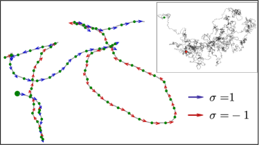
Figure 1: A typical trajectory of a DRABP generated by discretizing (1), where in a small interval $\Delta t,$ the particle reverses the direction with probability $\gamma\Delta t$ and with probability $1-\gamma\Delta t$ performs an ABP: $\{\Delta x(t),\Delta y(t)\}=v_{0}\sigma(t)\Delta t\{\cos\theta(t),\sin\theta(t)\};\,\Delta\theta(t)=\sqrt{2D_{R}\Delta t}\,\chi$, where $\chi$ is drawn from a standard normal distribution. The arrows indicate the instantaneous velocity vectors. The inset shows a long-time trajectory [which resembles a Brownian trajectory] with the two end-points marked. See SM for an animation.

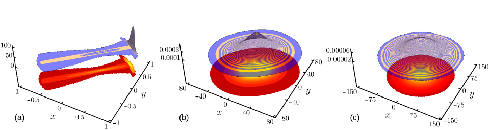
Figure 2: Dynamical evolution of the position distribution $P(x,y,t)$ for the case $\gamma>D_{R}$ obtained from numerical simulations. Here we have taken $\gamma=0.1$, $D_{R}=0.01$ and initial orientation $\theta_{0}=\pi/4.$ The panels (a), (b) and (c) correspond to $t=1$ [regime (I)], $t=50$ [regime (II)] and $t=200$ [regime (IV)], respectively. The strong anisotropy in regime (I) persists in the intermediate regime (II) eventually disappearing at large times (IV). See SM for a movie. For $\gamma<D_{R}$ the intermediate regime (b) is replaced by regime (III) which looks similar to (c).

In two dimensions, the position $\bm{x}=(x,y)$ and orientation $\theta$ of a DRABP evolve according to the Langevin equations,

$$\dot{x}(t) =v_{0}\,\sigma(t)\cos\theta(t)\equiv\zeta_{x}(t),$$ (1a)

$$\dot{y}(t) =v_{0}\,\sigma(t)\sin\theta(t)\equiv\zeta_{y}(t),$$ (1b)

$$\dot{\theta}(t) =\sqrt{2D_{R}}~{}\eta(t),$$ (1c)

where $D_{R}$ is the rotational diffusion coefficient, $\eta(t)$ is a Gaussian white noise with $\langle\eta(t)\rangle=0$ and $\langle\eta(t)\eta(t^{\prime})\rangle=\delta(t-t^{\prime}).$ The dichotomous noise $\sigma(t)$ alternates between $\pm 1$ at a constant rate $\gamma,$ triggering the direction reversal [see Fig. 1 for a typical trajectory].

In this Letter, we show that the presence of the two time-scales, $D_{R}^{-1}$ and $\gamma^{-1}$, gives rise to four distinct dynamical regimes: (I) $t\ll\min(\gamma^{-1},D_{R}^{-1}),$ (II) $\gamma^{-1}\ll t\ll D_{R}^{-1}$, (III) $D_{R}^{-1}\ll t\ll\gamma^{-1}$, and (IV) $t\gg\max(\gamma^{-1}$, $D_{R}^{-1})$, each characterized by a different dynamical behavior. Indeed, for Myxococcus xanthus, the well-separated time-scales ($\gamma^{-1}\simeq 10^{2}$ s and $~{}D_{R}^{-1}\simeq 10^{6}$ s  xanthustime ) make the regimes (I), (II) and (IV) experimentally accessible. We find that the position distribution shows a crossover from a strongly non-diffusive and anisotropic behavior at short-times to an eventual isotropic diffusive behavior via an intermediate regime (II) or (III) whose behaviors are very different. In regime (I), starting from the origin with a fixed orientation $\theta_{0}$, the position distribution of a DRABP is strongly anisotropic and shows a plateau-like structure around the origin accompanied by a single peak near $v_{0}t$ along $\theta_{0}$ [Figs. 2(a) and 3(a)]. For $\gamma>D_{R}$ the anisotropy persists in the intermediate time regime (II), however, with a peak at the origin [Fig. 2(b)]. In particular, we show that, the position distribution along the direction orthogonal to the initial orientation has a scaling form

$$P(x_{\perp},t)=\frac{1}{v_{0}t}\sqrt{\frac{\gamma}{8D_{R}}}f\left(\frac{x_{\perp}}{v_{0}t}\sqrt{\frac{\gamma}{8D_{R}}}\right),$$ (2)

with an exact non-trivial scaling function,

$$f(z)=\frac{1}{\sqrt{2\pi^{3}}}\Gamma\left(\frac{1}{4}+iz\right)\Gamma\left(\frac{1}{4}-iz\right),$$ (3)

where $\Gamma(z)$ is the gamma function. The tails of $f(z)$ decay exponentially [Fig. 3(b)]. Regime (III) appears for $D_{R}>\gamma$ where the distribution is Gaussian [Fig. 3(c)] with the variance $v_{0}^{2}/(2D_{R})$. The distribution is also a Gaussian in the late-time regime (IV), albeit with a different variance $v_{0}^{2}/[2(2\gamma+D_{R})]$ [Figs. 2(c) and 3(d)].

The persistence property also shows distinct behaviors in the four dynamical regimes (I)–(IV). We show that the directions parallel and orthogonal to the initial orientation are characterized by different persistence exponents, $\alpha_{\parallel}$ and $\alpha_{\perp}$ respectively, which are summarized in Table 1. The most noteworthy is a new persistence exponent $\alpha_{\perp}=1$ in the intermediate regime (II), emerging due to the presence of the direction reversal. In particular, in the limit $\gamma\to\infty$ and $D_{R}\to 0$, the first-passage time distribution for the perpendicular component has the scaling form

$$F_{\perp}(t;x_{\perp 0})=\frac{x_{\perp 0}\,\sqrt{2}\gamma^{3/2}}{v_{0}^{3}\,t^{2}\sqrt{D_{R}}}f\left(\frac{x_{\perp 0}}{v_{0}t}\sqrt{\frac{\gamma}{8D_{R}}}\right),$$ (4)

where $f(z)$ is given by Eq. (3) and $x_{\perp 0}$ is the initial position. In fact, for $\gamma>D_{R}$, we find that, $\alpha_{\perp}$ shows a non-monotonic behavior— $\alpha_{\perp}=1/4$ at short-times (I), which crosses over to $\alpha_{\perp}=1$ in the regime (II), and finally reaches the Brownian value $\alpha_{\perp}=1/2$ at late times (IV).

Position distribution.— We begin by considering the position distribution. The correlated nature of the effective noises $\zeta_{x,y}(t)$ in Eq. (1) makes the dynamics non-diffusive and anisotropic at short-times [see Sec. I of Supplemental Material SM for details]. In the following we first consider the two extreme regimes (I) and (IV) before coming to the intermediate regimes (II) and (III). We set $x(0)=y(0)=0$ without any loss of generality.

Short-time regime (I): Starting from the initial orientation $\theta(0)=\theta_{0}$ and $\sigma(0)=1,$ for $t\ll D_{R}^{-1}$ the effective noises can be approximated as,

$$\zeta_{x}(t)\approx v_{0}\sigma(t)(\cos\theta_{0}-\phi(t)\sin\theta_{0}),$$ (5a)

$$\zeta_{y}(t)\approx v_{0}\sigma(t)(\sin\theta_{0}+\phi(t)\cos\theta_{0}),$$ (5b)

where $\phi(t)=\sqrt{2D_{R}}\int_{0}^{t}\eta(s)\,ds$ denotes a standard Brownian motion. Here we have approximated $\cos\phi(t)\simeq 1$ and $\sin\phi(t)\simeq\phi(t)$ for $t\ll D_{R}^{-1}$ as $\phi(t)\sim\sqrt{D_{R}t}\ll 1$ abp2018 .

To obtain the marginal position distributions $P(x,t)$ and $P(y,t)$ corresponding to Eqs. (5), we adopt a trajectory based approach. The trajectory of the DRABP over a time-interval $[0,t]$ can be divided into $(n+1)$ intervals, punctuated by $n$ direction reversals; $\sigma$ remains constant between two consecutive reversals. We show that, for a specific sequence of intervals with duration $\{s_{1},s_{2},\dotsc,s_{n+1}\},$ the distribution of the final position $x$ is a Gaussian with mean $\cos\theta_{0}\sum_{i=1}^{n+1}(-1)^{i}s_{i}$ and variance $b_{n}\,\sin^{2}\theta_{0}$, where

$$b_{n}=2D_{R}\sum_{i=1}^{n+1}\Bigg{[}\sum_{j=1}^{i-1}(-1)^{i+j}s_{i}s_{j}(t_{j}+t_{j-1})+\frac{s_{i}^{2}}{3}(t_{i}+2t_{i-1})\Bigg{]}.$$

Here $t_{i}=\sum_{j=1}^{i}s_{j}$ with $t_{0}=0$ and $t_{n+1}=t.$ The position distribution is then obtained by taking weighted contributions from all such trajectories. Skipping details (Sec. III of SM ), we get,

$$P(x,t)= \frac{e^{-\gamma t}}{v_{0}\sin\theta_{0}\sqrt{2\pi}}\sum_{n=0}^{\infty}\gamma^{n}\int_{0}^{t}\prod_{i=1}^{n+1}ds_{i}\frac{\delta(t-\sum_{i=1}^{n+1}s_{i})}{\sqrt{b_{n}}}$$

$$\times\exp{\left[-\frac{(x+v_{0}\cos\theta_{0}\sum_{i=1}^{n+1}(-1)^{i}s_{i})^{2}}{2v_{0}^{2}\sin^{2}\theta_{0}b_{n}}\right]},$$ (6)

where each term corresponds to trajectories with a fixed number $n$ of reversals. We also obtain the $y$-marginal distribution $P(y,t)$ in the same manner, whose explicit form is given in SM .

Equation (6) provides the exact time-dependent marginal distribution for the process (5). Even though the infinite series cannot be summed explicitly to obtain a closed-form expression, it can be systematically evaluated numerically to obtain $P(x,t)$ for arbitrary $\gamma$ and $t.$ In fact, for $t\lesssim\gamma^{-1},$ it suffices to consider the first few terms to get a reasonably good estimate of the marginal distributions SM . Figure 3(a) compares this estimate, evaluated up to $n=2$ terms, with $P(x,t)$ obtained from numerical simulations. Clearly, this perturbative approach is extremely successful in accurately predicting the characteristic shape of the distribution, with a wide plateau near the origin and a peak near $x=v_{0}t$, in this short-time regime (I).

Physically, the peak in the distribution is a manifestation of the ABP nature of the motion—the $n=0$ term, corresponding to the no reversal case, correctly predicts the peak. The emergence of the plateau, however, is a direct consequence of the reversal events—for $t\ll D_{R}^{-1},$ the orientation $\theta$ evolves slowly, and the dynamics can be thought of as a one-dimensional RTP with an effective velocity $v_{0}\cos\theta_{0}.$ Now, for small values of $\gamma,$ the trajectories with a single flip contribute a constant value (the plateau) ${\gamma e^{-\gamma t}}/(2v_{0}\cos\theta_{0})$. This agrees well with the exact result [Eq. (6)] to leading order in $\gamma.$ Interestingly, such a plateau with a boundary-peak has been observed for motile bacteria in emulsion droplets plateau_experiment .

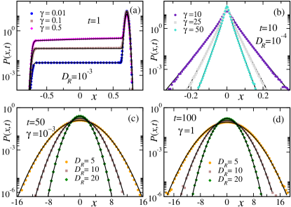
Figure 3: Marginal position distribution $P(x,t)$ in the different dynamical regimes: (a) $t\ll\min(D_{R}^{-1},\gamma^{-1})$, (b) $\gamma^{-1}\ll t\ll D_{R}^{-1}$, (c) $D_{R}^{-1}\ll t\ll\gamma^{-1}$, (d) $t\gg\max(D_{R}^{-1},\gamma^{-1})$. The symbols are from numerical simulations while solid black lines correspond to the analytical predictions given by Eqs. (6) [up to $n=2$],  (2), (8) and  (7) for (a)-(d) respectively. Here $v_{0}=1$ and we have used initial orientation $\theta_{0}=\pi/4$ for (a), (c) and (d) and $\theta_{0}=\pi/2$ for (b).

The anisotropic nature of the distribution in this short-time regime is a direct artifact of the fixed initial orientation. If, instead, the initial orientation is chosen uniformly, the position distribution becomes isotropic and an additional peak emerges at the origin (Fig. 3 of SM ).

Long-time regime (IV): For a given time $t$, mathematically, this regime can be accessed by taking both $D_{R}$ and $\gamma$ large ($\gg t^{-1}$). For large $D_{R}$ and arbitrary $\gamma$, the effective-noise autocorrelation becomes (Sec. II of SM ), $\langle\zeta_{a}(t)\zeta_{b}(t^{\prime})\rangle\approx 2D_{\text{eff}}\delta_{a,b}\,[D_{R}+2\gamma]\exp\bigl{(}-[D_{R}+2\gamma]|t-t^{\prime}|\bigr{)}$ where $2D_{\text{eff}}=v_{0}^{2}/{(D_{R}+2\gamma)}$. Thus in the limit $D_{R},\gamma\to\infty$, it tends to $2D_{\text{eff}}\delta_{a,b}\delta(t-t^{\prime})$ which results in the isotropic Gaussian distribution,

$$P(x,y,t) \approx \frac{1}{2D_{\text{eff}}t}G\left(\frac{x}{\sqrt{2D_{\text{eff}}t}},\frac{y}{\sqrt{2D_{\text{eff}}t}}\right),$$ (7)

with $G(\tilde{x},\tilde{y})=e^{-(\tilde{x}^{2}+\tilde{y}^{2})/2}/(2\pi)$. The corresponding $x$-marginal distribution (which, obviously, is also a Gaussian) is plotted in Fig. 3(d) along with the data from numerical simulations; an excellent agreement validates our prediction.

Intermediate-time regime (III): This regime corresponds to $D_{R}\gg t^{-1}\gg\gamma$, where $\langle\zeta_{a}(t)\zeta_{b}(t^{\prime})\rangle\to(v_{0}^{2}/D_{R})\delta_{a,b}\,\delta(t-t^{\prime}).$ Therefore, the typical position distribution is again Gaussian with the width $v_{0}\sqrt{t/D_{R}}$,

$$P(x,y,t)\approx\frac{D_{R}}{v_{0}^{2}t}\,G\left(\frac{x}{v_{0}\sqrt{t/D_{R}}},\frac{y}{v_{0}\sqrt{t/D_{R}}}\right),~{}$$ (8)

with $G(\tilde{x},\tilde{y})=e^{-(\tilde{x}^{2}+\tilde{y}^{2})/2}/(2\pi).$ Note that this result is same as in the case of ABP for $t\gg D_{R}^{-1}$ abp2018 —adding directional reversal does not change the physical scenario in this regime. We validate this prediction with numerical simulations in Fig. 3(c).

Intermediate-time regime (II): The correlated noise leads to an intriguing behavior in this regime $\gamma^{-1}\ll t\ll D_{R}^{-1}.$ For $t\gg\gamma^{-1},$ the frequent reversals lead to a Gaussian white noise $\xi(t)$ with zero-mean and the correlator $\langle\xi(t)\xi(t^{\prime})\rangle=\gamma^{-1}\delta(t-t^{\prime})$. Thus, for $t\ll D_{R}^{-1}$, from Eqs. (5), the effective noises can be approximated as,

$$\zeta_{x}(t) \approx v_{0}\,\xi(t)(\cos\theta_{0}-\phi(t)\sin\theta_{0}),$$ (9a)

$$\zeta_{y}(t) \approx v_{0}\,\xi(t)(\sin\theta_{0}+\phi(t)\cos\theta_{0}).$$ (9b)

Equations (9) describe a Brownian motion with stochastically evolving diffusion coefficients. Some specific versions of such models have been studied recently diffusing_diff in a different context.

The Gaussian nature of $\xi(t)$, for a fixed $\{\phi(s)\}$ trajectory, allows us to evaluate the characteristic function, $\langle e^{i\bm{k}\cdot\bm{x}}\rangle=\left\langle\exp{\left[-\frac{1}{2}\bm{k}^{\text{T}}\,\bm{\Sigma}(t)\,\bm{k}\right]}\right\rangle_{\phi},$ where $\bm{k}=\left({k_{x},k_{y}}\right)^{\text{T}}$ and ${\bm{\Sigma}}(t)$ is the correlation matrix whose explicit form is given in Sec. IV of SM . The subscript $\phi$ denotes averaging over the Brownian paths $\{\phi(s)\}$, which can be performed using path integral approach. This yields SM ,

$$\langle e^{i\bm{k}\cdot\bm{x}}\rangle=\frac{1}{\sqrt{\cosh\omega t}}\exp\left[-\frac{\omega\tanh\omega t}{4D_{R}}\left(\frac{k_{x}+k_{y}\tan\theta_{0}}{k_{y}-k_{x}\tan\theta_{0}}\right)^{2}\right],$$

(10)

where $\omega=v_{0}\sqrt{{2D_{R}}/{\gamma}}\,(k_{y}\cos\theta_{0}-k_{x}\sin\theta_{0}).$ Of particular interest are the distributions along and orthogonal to the initial orientation, denoted by $x_{\parallel}$ and $x_{\perp}$ respectively. Setting $\theta_{0}=0$ gives $x_{\perp}\equiv y$ and $x_{\parallel}\equiv x$.

Putting $k_{x}=0,\,k_{y}=k$ in Eq. (10), yields $\langle e^{ikx_{\perp}}\rangle=\left[\cosh\left(v_{0}kt\sqrt{{2D_{R}}/{\gamma}}\right)\right]^{-\frac{1}{2}}$, which leads to the non-trivial distribution announced in Eqs. (2)-(3) for $x_{\perp}$. Figure 3(b) shows an excellent agreement between Eq. (3) and the numerical simulations. The tails of the distribution decay as $\sim\exp[-\pi|x_{\perp}|/(2\sqrt{2}\ell)]$, where the charachteristic length-scale $\ell=v_{0}t\sqrt{D_{R}/\gamma}$ is the root-mean-square displacement (Eq. 14 in SM) in regime (II). It is evident from the ballistic scaling form Eq. (2) that the variance $\propto t^{2}$ (Eq. (14) in SM ). On the other hand, $k_{y}=0,\,k_{x}=k$ gives $\langle e^{ikx_{\parallel}}\rangle=e^{-v_{0}^{2}k^{2}\,t/(2\gamma)}$, which leads to a Gaussian distribution with a variance $v_{0}^{2}t/\gamma$, indicating diffusive fluctuations. This drastically different nature of the fluctuations for $x_{\perp}$ and $x_{\parallel}$ leads to the anisotropic distribution seen in Fig. 2 (b).

First-passage properties.— We next consider the survival probability which is the cumulative distribution of the first-passage time. We set $\theta_{0}=0$ so that $x_{\parallel}=x$ and $x_{\perp}=y$. Let $S_{y}(t;y_{0})$ denote the probability that, starting from some arbitrary position $y(0)=y_{0}$ the $y$-component of the position has not crossed the $y=0$ line up to time $t$; $S_{x}(t;x_{0})$ is defined similarly.

The most interesting scenario appears for $\gamma>D_{R}$ where $S_{y}(t)$ shows three distinct persistence behaviors in the three different dynamical regimes. For $\theta_{0}=0$, Eq. (5b) leads to $\dot{y}=v_{0}\sigma(t)\phi(t)$. Now, for $t\ll\gamma^{-1}$, this can be approximated as a random acceleration process $\dot{y}\simeq v_{0}\sigma(0)\phi(t)$, for which the persistence exponent is $1/4$ rap1 ; rap2 . Therefore, in the short-time regime (I), we expect $\alpha_{y}=1/4$, which is verified in Fig. 4(a) using numerical simulations.

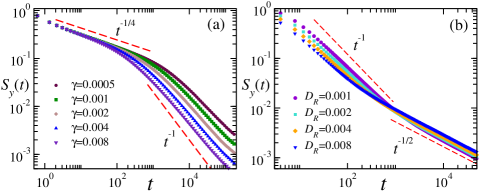
Figure 4: $S_{y}(t)$ vs $t$ for $\gamma>D_{R}$: (a) shows the crossover from $\alpha_{y}=1/4$ (I) to $\alpha_{y}=1$ (II) for a fixed $D_{R}=10^{-5}$ and $y_{0}=0.001.$ (b) shows the crossover from $\alpha_{y}=1$ (II) to $\alpha_{y}=1/2$ (IV) for $\gamma=1$ and $y_{0}=0.1$.

In the intermediate time regime (II) the effective $y$-dynamics [see (9b)] becomes $\dot{y}=v_{0}\xi(t)\phi(t)$ for $\theta_{0}=0.$ We compute the survival probability by solving the corresponding Fokker Planck equation with an absorbing boundary condition at $y=0$. This leads to a new persistence exponent $\alpha_{y}=1$ in the context of active particles. In fact, in the limit $\gamma\to\infty$ and $D_{R}\to 0$, we find the exact first-passage time distribution Eq. (4), which we verify using numerical simulations in Sec. V of SM . This result is consistent with the recently obtained first-passage behavior for the diffusing diffusivity model fpt_DD . We show the crossover from $\alpha_{y}=1/4$ to $\alpha_{y}=1$ near $t\sim\gamma^{-1}$ using numerical simulations in Fig. 4(a).

In the large time regime (IV), as discussed earlier, the particle behaves like an ordinary diffusion process with an effective diffusion constant. Consequently, the survival probability decays with the Brownian exponent $\alpha_{y}=1/2$ as seen from the numerical simulations in Fig. 4(b). The crossover from $\alpha_{y}=1$ to $\alpha_{y}=1/2$ occurs around $t\sim D_{R}^{-1}$.

If $D_{R}>\gamma$, we effectively see two distinct exponents $\alpha_{y}=1/4$ in the short-time regime (I), which crosses over to $\alpha_{y}=1/2$ in regime (III) and remains the same for large times (IV). We also study $S_{x}(t)$ which shows Brownian behavior at all times except in regime (I), where $\alpha_{x}=0$ due to the fact that the particle always survives for $t\ll\gamma^{-1}$; see Fig. 6 in SM . A summary of the exponents in all the regimes is provided in Table 1.

Persistence Exponent	I	II	III	IV
$\alpha_{\perp}$	$1/4$	$1$	$1/2$	$1/2$
$\alpha_{\parallel}$	$0$	$1/2$	$1/2$	$1/2$

Table 1: Persistence exponents for the $x_{\perp}$ and $x_{\parallel}$ components of the DRABP as defined by decay of the survival probability $S(t)\sim t^{-\alpha}$ in the different dynamical regimes: (I) $t\ll\min(D_{R}^{-1},\gamma^{-1}),$ (II) $\gamma^{-1}\ll t\ll D_{R}^{-1},$ (III) $D_{R}^{-1}\ll t\ll\gamma^{-1},$ and (IV) $t\gg\max(\gamma^{-1},D_{R}^{-1}).$

In conclusion, we provide a comprehensive analytical understanding of the DRABP that models a wide range of bacterial motion. The DRABP shows many novel features — the presence of the direction reversal along with rotational diffusion gives rise to four distinct dynamical regimes each of which corresponds to a different position distribution and persistence exponent. In particular, we find that, the position distribution in the short-time and intermediate-time regimes have certain unique features, very different from ordinary ABP and RTP. The short-time regime is characterized by the emergence of a plateau. The intermediate regime $\gamma^{-1}\ll t\ll D_{R}^{-1}$ shows a unique scaling behavior [see Eqs. (2)-(3)]. We also find a novel persistence exponent $\alpha=1$, which have not been seen in active motions so far, in the same regime.

Our work opens up the possibility to explore a wide range of problems in the study of active motions, both experimentally and theoretically. Our results for the position distribution may be verified in experiments with dilute solutions of bacteria xanthus2 ; putida2 or artificial active colloids Verman2020 . Moreover, it would be really interesting to observe the non-monotonic persistence exponent behavior from single particle tracking. In this Letter we have considered the direction reversal to be a Poisson process. To study the effect of other reversal-time distributions, like Gamma-distributions grossman1 ; detcheverry or a power-law, is a challenging open question. It would also be interesting to study the effect of interaction on DRABP, which would help understand the complex phenomena seen in experiments xanthusagg1 ; xanthusagg2 .

- (1) P. Romanczuk, M. Bar, W. Ebeling, B. Lindner, and L. Schimansky-Geier, Active Brownian Particles. From Individual to Collective Stochastic Dynamics, Eur. Phys. J. Special Topics 202, 1 (2012).
- (2) M. C. Marchetti, J. F. Joanny, S. Ramaswamy, T. B. Liverpool, J. Prost, Madan Rao, and R. Aditi Simha, Hydrodynamics of soft active matter, Rev. Mod. Phys. 85, 1143 (2013).
- (3) G. S. Redner, M. F. Hagan, and A. Baskaran, Structure and Dynamics of a Phase-Separating Active Colloidal Fluid, Phys. Rev. Lett. 110, 055701 (2013).
- (4) Y. Fily, A. Baskaran and M. F. Hagan, Activity-Induced Phase Separation and Self-Assembly in Mixtures of Active and Passive Particles , Soft Matter 10, 5609 (2014).
- (5) J. Schwarz-Linek, C. Valeriani, A. Cacciuto, M. E. Cates, D. Marenduzzo, A. N. Morozov and W. C. K. Poon, Phase separation and rotor self-assembly in active particle suspensions, Proc. Natl. Acad. Sci. USA 109, 4052 (2012).
- (6) G. Gompper, R. G Winkler, T. Speck, A. Solon, C. Nardini, F. Peruani, H. Lowen, R. Golestanian, U. Benjamin Kaupp, L. Alvarez et. al., The 2020 motile active matter roadmap, J. Phys.: Condens. Matter 32, 193001 (2020).
- (7) S. Ramaswamy, Active matter, J. Stat. Mech. 054002 (2017).
- (8) J. Stenhammar, R. Wittkowski, D. Marenduzzo, and M. E. Cates, Activity-Induced Phase Separation and Self-Assembly in Mixtures of Active and Passive Particles, Phys. Rev. Lett. 114, 018301 (2015).
- (9) A. P. Solon, Y. Fily, A. Baskaran, M. E. Cates, Y. Kafri, M. Kardar, J. Tailleur, Pressure is not a state function for generic active fluids, Nature Phys. 11, 673 (2015).
- (10) C. Bechinger, R. Di Leonardo, H. Lowen, C. Reichhardt, G. Volpe and G. Volpe, Active particles in complex and crowded environments, Rev. Mod. Phys. 88, 045006 (2016).
- (11) J. Tailleur and M. E. Cates, Statistical Mechanics of Interacting Run-and-Tumble Bacteria, Phys. Rev. Lett. 100, 218103 (2008).
- (12) C. Kurzthaler, S. Leitmann and T. Franosch, Intermediate scattering function of an anisotropic active Brownian particle, Scientific Reports 6, 36702 (2016).
- (13) T. Demaerel, C. Maes, Active Processes in 1D, Phys. Rev. E 97, 032604 (2018).
- (14) A. Dhar, A. Kundu, S. N. Majumdar, S. Sabhapandit, G. Schehr, Run-and-tumble particle in one-dimensional confining potentials: Steady-state, relaxation, and first-passage properties, Phys. Rev. E 99, 032132 (2019).
- (15) W. Stadje, The exact probability distribution of a two-dimensional random walk, J. Stat. Phys. 46, 207 (1987).
- (16) K. Malakar, V. Jemseena, A. Kundu, K. Vijay Kumar, S. Sabhapandit, S. N. Majumdar, S. Redner, A. Dhar, Steady state, relaxation and first-passage properties of a run-and-tumble particle in one-dimension, JSTAT 043215 (2018).
- (17) I. Santra, U. Basu, S. Sabhapandit, Run-and-tumble particles in two dimensions: Marginal position distributions, Phys. Rev. E 101, 062120 (2020).
- (18) F. Mori, P. L. Doussal, S. N. Majumdar, and G. Schehr, Universal Survival Probability for a d-Dimensional Run-and-Tumble Particle, Phys. Rev. Lett. 124, 090603 (2020).
- (19) F. J. Sevilla and L. A. G. Nava, Theory of diffusion of active particles that move at constant speed in two dimensions Phys. Rev. E90, 022130 (2014).
- (20) S. N. Majumdar and B. Meerson, Toward the full short-time statistics of an active Brownian particle on the plane, Phys. Rev. E 102, 022113 (2020).
- (21) A. Pototsky and H. Stark, Active Brownian particles in two-dimensional traps, EPL 98, 50004 (2012).
- (22) U. Basu, S. N. Majumdar, A. Rosso, G. Schehr, Active Brownian motion in two dimensions, Phys. Rev. E 98, 062121 (2018).
- (23) U. Basu, S. N. Majumdar, A. Rosso, G. Schehr, Long-time position distribution of an active Brownian particle in two dimensions, Phys. Rev. E 100, 062116 (2019).
- (24) K. Malakar, A. Das, A. Kundu, K. V. Kumar, A. Dhar, Steady State of an Active Brownian Particle in Two-Dimensional Harmonic Trap, Phys. Rev. E 101, 022610 (2020).
- (25) A. Shee, A. Dhar and D. Chaudhuri, Active Brownian particles: mapping to equilibrium polymers and exact computation of moments, Soft Matter 16, 4776 (2020).
- (26) H.C. Berg, Random walks in biology, (Princeton University Press, New Jersey, 1993).
- (27) J. R. Howse, R. A. L. Jones, A. J. Ryan, T. Gough, R. Vafabakhsh, R. Golestanian, Self-Motile Colloidal Particles: From Directed Propulsion to Random Walk, Phys. Rev. Lett. 99, 048102 (2007).
- (28) S. C. Takatori, R. De Dier, J. Vermant, and J. F. Brady, Acoustic trapping of active matter , Nature Comm. 7, 10694 (2016).
- (29) Y. Wu, A. D. Kaiser, Y. Jiang and M. S. Alber, Periodic reversal of direction allows Myxobacteria to swarm, Proc. Natl. Acad. Sci., USA 106, 1222 (2009).
- (30) S. Thutupalli, M. Sun, F. Bunyak, K. Palaniappan and J. W. Shaevitz, Directional reversals enable Myxococcus xanthus cells to produce collective one-dimensional streams during fruiting-body formation, J. R. Soc. Interface 12, 20150049 (2015).
- (31) S. Leonardy, I. Bulyh, and L. S-Andersen, Reversing cells and oscillating motilityproteins, Mol. BioSyst. 4, 1009 (2008).
- (32) G. Liu, A. Patch, F. Bahar, D. Yllanes, R. D. Welch, M. C. Marchetti, S. Thutupalli, and J. W. Shaevitz, Self-Driven Phase Transitions Drive Myxococcus xanthus Fruiting Body Formation, Phys. Rev. Lett. 122, 248102 (2019).
- (33) C. S. Harwood, K. Fosnaugh and M. Dispensa, Flagellation of Pseudomonas putida and analysis of its motile behavior, J. Bacteriol., 171, 4063 (1989).
- (34) M. Theves, J. Taktikos, V. Zaburdaev, H. Stark, and C. Beta, A bacterial swimmer with two alternating speeds of propagation, Biophys J. 105, 1915 (2013).
- (35) J. E. Johansen, J. Pinhassi, N. Blackburn, U. L. Zweifel and A. Hagström, Variability in motility characteristics among marine bacteria, Aquat. Microb. Ecol. 28, 229 (2002).
- (36) G. M. Barbara, J. G. Mitchell, Bacterial tracking of motile algae, FEMS Microbiology Ecology, 44, 79 (2003).
- (37) B. L. Taylor and D. E. Koshland, Reversal of flagellar rotation in monotrichous and peritrichous bacteria: generation of changes in direction, J. Bacteriol., 119, 640 (1974).
- (38) U. Börner, A. Deutsch, H. Reichenbach, and M. Bär, Rippling Patterns in Aggregates of Myxobacteria Arise from Cell-Cell Collisions, Phys. Rev. Lett. 89, 078101 (2002).
- (39) O. Sliusarenko, J. Neu, D. R. Zusman, G. Oster, Myxobacteria: Moving, Killing, Feeding, and Surviving Together, Proc. Nat. Ac. Sc. USA 103, 1534 (2006).
- (40) M. Gjermansen, Paula Ragas, Claus Sternberg, S. Molin and T. Tolker-Nielsen, Characterization of starvation-induced dispersion in Pseudomonas putida biofilms, Environ. Microbiol. 7, 894 (2005).
- (41) S. Redner, A Guide to First-Passage Processes, Cambridge University Press (2001).
- (42) A. J. Bray, S. N. Majumdar, and G. Schehr, Persistence and First-Passage Properties in Non-equilibrium Systems, Adv. Phys. 62, 225 (2013).
- (43) O. Sliusarenko, D. R. Zusman, and G. Oster, Aggregation during Fruiting Body Formation in Myxococcus xanthus Is Driven by Reducing Cell Movement, J. Bacteriol. 189, 611 (2007).
- (44) See Supplemental Material for details which includes Refs. fpt_DD , grossman1 -dlmf .
- (45) I. D. Vladescu, E. J. Marsden, J. Schwarz-Linek, V. A. Martinez, J. Arlt, A. N. Morozov, D. Marenduzzo, M. E. Cates, and W. C. K. Poon, Filling an Emulsion Drop with Motile Bacteria, Phys. Rev. Lett. 113, 268101 (2014).
- (46) V. Sposini, D. S. Grebenkov, R. Metzler, G. Oshanin and F. Seno, Universal spectral features of different classes of random-diffusivity processes, New J. Phys. 22, 063056 (2020).
- (47) T. W. Burkhardt, Semiflexible polymer in the half plane and statistics of the integral of a Brownian curve, J. Phys. A: Math. Gen. 26 L1157 (1993).
- (48) T. W. Burkhardt, Dynamics of absorption of a randomly accelerated particle, J. Phys. A: Math. Gen. 33 L429 (2000).
- (49) D. S. Grebenkov, V. Sposini, R. Metzler, G. Oshanin and F. Seno, Exact first-passage time distributions for three random diffusivity models J. Phys. A: Math. Theor. 54, 04LT01 (2020).
- (50) H. R. Vutukuri, M. Lisicki, E. Lauga, and J. Vermant, Light-switchable propulsion of active particles with reversible interactions, Nat. Comm. 11, 2628 (2020).
- (51) F. Detcheverry, Generalized run-and-turn motions: From bacteria to Lévy walks, Phys. Rev. E 96, 012415 (2017).
- (52) R. Großmann, F. Peruani and M. Bär, Diffusion properties of active particles with directional reversal, New J. Phys. 18, 043009 (2016).
- (53) S. N. Majumdar, Current Science, Brownian Functionals in Physics and Computer Science 89, 2076 (2005).
- (54) R. P. Feynman, A. R. Hibbs, Quantum Mechanics and Path Integrals, McGraw-Hill, New York (1965).
- (55) NIST Digital Library of Mathematical Functions, F. W. J. Olver, A. B. Olde Daalhuis, D. W. Lozier, B. I. Schneider, R. F. Boisvert, C. W. Clark, B. R. Miller, B. V. Saunders, H. S. Cohl, and M. A. McClain, https://dlmf.nist.gov/.