Demographic feedbacks can hamper the spatial spread of a gene drive
Abstract.
This paper is concerned with a reaction–diffusion system modeling the fixation and the invasion in a population of a gene drive (an allele biasing inheritance, increasing its own transmission to offspring). In our model, the gene drive has a negative effect on the fitness of individuals carrying it, and is therefore susceptible of decreasing the total carrying capacity of the population locally in space. This tends to generate an opposing demographic advection that the gene drive has to overcome in order to invade. While previous reaction–diffusion models neglected this aspect, here we focus on it and try to predict the sign of the traveling wave speed. It turns out to be an analytical challenge, only partial results being within reach, and we complete our theoretical analysis by numerical simulations. Our results indicate that taking into account the interplay between population dynamics and population genetics might actually be crucial, as it can effectively reverse the direction of the invasion and lead to failure. Our findings can be extended to other bistable systems, such as the spread of cytoplasmic incompatibilities caused by Wolbachia.
Key words and phrases:
population genetics, population dynamics, gene drive, traveling wave, bistability.2010 Mathematics Subject Classification:
35K57, 92D10, 92D25.1. Introduction
1.1. Biological background
Some genetic elements can bias inheritance in their favor, and therefore spread in a population over successive generations, even if they are costly to the organism carrying them [40], a phenomenon called gene drive [1]. Inspired from natural systems, synthetic gene drives have been developed over the last decades for the control of natural populations [33]. Artificial gene drives can be used to spread a genetic modification in a natural population [8], in order to (i) modify this target population (for instance, make disease vectors resistant to the pathogen that they transmit) without significantly affecting its size (replacement drives), or (ii) reduce the size of the target population by spreading an allele that affects fecundity or survival (suppression drives), or even eradicate the target population (eradication drives) [12] .
One way of biasing transmission involves copying the drive element onto the other chromosome in heterozygous cells [7], a process called gene conversion or “homing”. A target sequence on the other chromosome is recognized, cleaved, and a DNA-repair mechanism using the intact chromosome as a template leads to the duplication of the drive element. The drive element is then present in most gametes and therefore in most offspring. The high flexibility and programmability brought about by the CRISPR-Cas genome editing technology greatly simplifies the creation of this type of artificial gene drives [16], and has led to a renewed interest in this technique of population control.
To date, artificial gene drives have been confined to laboratory experiments; field trials, whether small-scale and confined, or open, have not taken place yet [15]. In between, mathematical models can help identify features of gene drives that are most important in determining their dynamics; models can also help anticipate potential issues, and are an essential step between lab and field experiments [27].
A key feature affecting the spread of gene drives is the existence or not of a release threshold. Some drive systems spread from arbitrary low introduction frequencies (“threshold-independent drives”), while some others only do if enough drive-carrying individuals are introduced in the population (“threshold-dependent drives” or “high-threshold drives”) [15, p19]. In mathematical terms, a release threshold corresponds to the existence of an unstable internal equilibrium (i.e., where wild-type and drive alleles coexist), in other words, of a bistability. Homing-based gene drives can belong to the two categories, depending on their intrinsic parameters [11].
The existence of a release threshold affects the spatial spread of a drive and the potential for spatial confinement. High-threshold drives can be spatially confined if dispersal is limited [2, 24, 21]. In spatially continuous environment, the shape of the wave of advance of a drive system changes from pulled for no-threshold drives to pushed in high-threshold drives [12]. A wave of advance of a high-threshold drive can be stopped by obstacles [36]. More generally, these results are in line with those of models of spatial spread of bistable systems [3, 4].
Many mathematical models of the spatial spread of gene drives focus on allele frequencies and ignore changes in population density. Changes in the size of the target population will however happen with the spread of a gene drive, either as a potential side effect for replacement drives, or as a feature for suppression and eradication drives. Considering these spatial and temporal variations in population size matters, because they create fluxes of individuals from more densely to less densely populated locations, opposing the spread of the gene drive [12].
Beaghton et al. [5] used a reaction–diffusion framework to study the spatial spread of a driving-Y chromosome causing population suppression or eradication, and explicitly followed population densities. In a driving-Y system, the offspring of driving-Y bearing males are almost all driving-Y bearing males, because the development of X-chromosome bearing gametes is disrupted. A driving-Y is a no-threshold drive: in a well-mixed population, a driving-Y system can increase from arbitrary low frequencies. Beaghton et al. showed that a driving-Y system would spread spatially, and they calculated the speed of the wave of advance.
In this article, we use a system of partial differential equations to study the spread of a homing-based gene drive over a one-dimensional space, explicitly taking into account changes in population sizes. In our model, the fitness cost associated to the drive affects the level of population suppression, but also the existence and value of the release threshold. We explore the model numerically and prove some results mathematically for large regions of the parameter space. We explore the robustness of our finding by considering other forms of density dependence (including Allee effects), assuming fitness effects on other fitness components, and finally extend our result to another bistable system, the spread of cytoplasmic incompatibilities brought about by Wolbachia.
1.2. Organization of the paper
In the rest of Section 1, we present our mathematical model, relate it to the literature, and state our results. In Section 2, we explain our numerical method and prove our analytical results. In Section 3, we conclude with a mathematical and biological discussion.
1.3. Derivation of the reaction–diffusion system
To derive our equations, we follow the methodology presented in [31]. In addition, we assume that heterozygous individuals are functionally equivalent to drive homozygotes. This can be the case when the conversion rate is , and either (i) gene conversion (also called homing) takes place early in development (typically in the zygote – as opposed to gene conversion in the germline) – so that heterozygotes are all immediately converted into homozygotes, and no heterozygous individuals are ever introduced to the population from an outside source, or (ii) gene conversion takes place later in the life cycle, but the drive is dominant, so that heterozygotes have the same fitness as drive homozygotes (and then only transmit the drive allele, since gene conversion is ) . This assumption simplifies a lot the model since we have to track two genotypes instead of three in general: in scenario i), there are never heterozygous individuals in the population, and in scenarion ii), heterozygotes can be conflated with drive homozygotes since they behave exactly the same way. This leads to the following reaction–diffusion system:
| (1) |
where:
-
•
and , nonnegative functions of time and space , are (continuous densities approximating) the number of alleles and respectively, or (up to a factor ) the number of homozygous individuals and respectively;
-
•
for each allele , is the spatial diffusion rate of homozygous individuals, is their juvenile survival rate (the proportion of newborns that survive until the adult age), is the fecundity rate of a gamete carrying (fecundity being defined here multiplicatively in the sense that a mating between and individuals will produce newborns), is the death rate of individuals, and all these parameters are positive constants;
-
•
and , nonnegative functions of the total population size, are the per capita birth rate and death rate. If they were positive constants, then a pure wild-type population would undergo exponential growth, which is not realistic; by using non-constant, a priori nonlinear, functions, we can model more complex population dynamics, like logistic growth or Allee effects.
Our assumptions of early and successful gene conversion (homing) are reflected in the presence of the term in the first equation of system (1); assuming late gene conversion and a dominant drive allele, together with gene conversion, results in the same equations.
Defining
we obtain the reduced system:
Assuming subsequently that selection does not act on mobility (), changing the variable into , and getting rid of all “” for ease of reading, we obtain the reduced system:
The biological meaning of the parameters in this simpler system is the following: , , are multiplicative variations to the “norm” fixed by individuals. For instance, if , then wild-type homozygotes () are twice more fecund than drive homozygotes ().
Finally, when selection only acts on survival with a fitness cost (, , standing assumptions from now on), the system reads:
| (2) |
Defining the total population density and the proportion of allele , we find that the equivalent system satisfied by is:
| (3) |
In the above system and in the whole paper, is the natural logarithm.
and are still unspecified at this point.
The equation for in system (3) has a non-trivial equilibrium , which is admissible when . In this case, this internal equilibrium is unstable. The release-threshold properties of the gene drive are therefore given by the value of : the drive is threshold-independent when , and threshold dependent when , the value of the release threshold being .
1.4. Carrying capacity and gene drive typology
A pure wild-type population is governed by the equation . Hence can be understood as the wild-type intrinsic growth rate per capita. Subsequently, we define the wild-type carrying capacity (i.e., equilibrium population size) as follows:
-
•
if for any , then the carrying capacity is ;
-
•
otherwise, the carrying capacity is the maximal value of for which .
For well-posedness purposes, we assume that the carrying capacity is finite, and without loss of generality we assume that it is , fixing the unit of population density111For any , the pair with birth and death rates and satisfies the same system as the pair with birth and death rates , . Hence the normalization can be done without loss of generality and all forthcoming results do not depend on the wild-type carrying capacity..
In a spatially homogeneous setting, a population goes extinct if, and only if, its carrying capacity is zero. The growth rate of a pure population is . Hence, in our framework,
-
•
corresponds to pure, costless, replacement drives;
-
•
as soon as , the drive is a suppression drive, lowering the carrying capacity of the population;
-
•
the necessary and sufficient condition for the drive to be an eradication drive, namely a drive whose carrying capacity is , is:
Finally, a simple rescaling of space and time shows that the pair and the pair , for any , lead to the same system. In order to fix the ideas, in what follows, the pair is normalized by the standing assumption .
1.5. Relations with other models from the literature
In the recent literature, reaction–diffusion models related to system (4) have attracted a special attention, be it for the study of gene drive or in other evolution or population genetics contexts 222The shared history between reaction–diffusion PDEs and population genetics is ancient: we remind the reader that both Fisher [17] and Kolmogorov, Petrovsky and Piskunov [23] introduced the equation that is now famously called the Fisher–KPP equation as a population genetics model.. Let us show how our model relates to some of those earlier models.
Fixing in the following discussion , system (4) becomes:
| (4) |
1.5.1. Deriving ref. [26, 20, 36] from system (4)
Recall that in this discussion, .
If is a positive constant (population subjected to pure, unrealistic, Malthusian growth), then up to a rescaling of , the equation on reads
| (5) |
Together with V. Calvez, we studied this equation in a gene drive context [20, Section 4.3] without a priori knowledge on . It has also been studied in a mosquito–Wolbachia context by Nadin, Strugarek and Vauchelet in [26].
Back to (4) with a non-constant function , recalling that the wild-type carrying capacity is (namely, ), we consider small variations about (a replacement drive) by defining a “rescaled total population” (i.e., ) and, following Strugarek–Vauchelet [35], we find
Formally, if with the scalings , , , , this system becomes
This limit can actually be made rigorous [35] provided:
-
•
the birth rate depends on the small parameter in such a way that can be rewritten as a function of only, i.e., ;
-
•
the time horizon is finite, or in other words, we are only concerned with the early gene drive dynamics, and not with its long-time asymptotic spreading.
It turns out that the latter equation on is exactly the equation studied in a gene drive spreading context by Tanaka–Stone–Nelson [36]:
| (6) |
Although Tanaka–Stone–Nelson’s paper [36] and Strugarek–Vauchelet’s paper [35] were published the same year and without direct knowledge one from another, they can therefore be related a posteriori: our general model reduces to Tanaka–Stone–Nelson’s model via Strugarek–Vauchelet’s limiting procedure in a context of replacement drives invading populations at carrying capacity, and Tanaka–Stone–Nelson’s model can be used to study spreading properties provided the Strugarek–Vauchelet limiting procedure remains valid with an infinite time horizon. In this regard, our paper can be understood as an investigation of the validity of the approximation (6) to study spreading properties and for suppression or eradication drives.
Back to system (4), it is formally clear that, under a weak selection assumption , the total population does not depend a lot on the allelic frequency , is close to the wild-type carrying capacity everywhere, and by virtue of , the equation on can be approximated by
| (7) |
This equation is both an approximation of (5) with and an approximation of (6) with . This formal reasoning illustrates in another way how our model is consistent with the model of Tanaka–Stone–Nelson [36] under a weak selection assumption 333It was precisely the aim of Strugarek and Vauchelet [35] to make such formal statements rigorous..
Finally, another variant might be
| (8) |
The difference with eq. (6) is the presence of the advection term . In our paper with V. Calvez [20], we also studied equation (8), without a priori knowledge on . It is not clear how this equation can be deduced from our current model and we leave this as an open problem – yet, in the next section we will explain how all these models descend from a unique discrete-time model. In any case, our intent there was to depart from the Tanaka–Stone–Nelson model and to introduce basic population density effects by means of this advection term. As such, this first work motivated the present one and this modeling clarification as well.
1.5.2. Deriving all models from a unique discrete-time one
Alternatively, we can derive all these models from a discrete-time model with non-overlapping generations [39, 11, 38].
To obtain (4), the operations have to be performed in the following order:
-
(1)
write the equations for and ;
-
(2)
subtract from it and respectively and perform a first-order Taylor expansion ;
-
(3)
add spatial diffusion to the equations;
-
(4)
then write the equivalent system satisfied by ; it is (4) indeed.
Going back to refs. [36, 20], we find that there the operations are performed in the following different order:
-
(1)
write the equations for and ;
-
(2)
write the equivalent system satisfied by ;
-
(3)
by Taylor expansion, write the continuous-time system satisfied by ;
- (4)
Although the obtained equation on remains the same as in (4), the equation on differs and is (6) or (8) (depending on whether the advection term was accounted for).
Let us highlight the fact that the two processes above lead to different systems and are not equivalent. Nevertheless, we pointed out in [20, Section 4.3] that the two systems have similar qualitative behaviors.
1.6. Main results
In what follows, we choose to focus, for the sake of exposition, on the simplest non-constant choice for and , namely a constant death rate with logistic wild-type growth: , . The parameter is the intrinsic growth rate of a wild-type population, or wild-type intrinsic growth rate for short (in the literature, intrinsic growth rates are also sometimes known as Malthusian growth rates). Thus we have two parameters in the model, the fitness cost and the wild-type intrinsic growth rate . We will discuss more complicated choices in Section 3.
The reaction–diffusion systems are:
| (9) |
| (10) |
For these systems, the eradication condition is .
Since we are concerned with spreading properties, and more precisely with the ability of the gene drive to invade a wild-type population when introduced in sufficiently high numbers in a confined area of space, we neglect boundary effects, assume that the physical space is a Euclidean space – to simplify even further, we assume it is the one-dimensional Euclidean space – and assume that the initial conditions are close to everywhere and in a sufficiently large compact interval.
1.6.1. Numerical results
All numerical simulations are performed in GNU Octave [14] using standard implicit finite difference schemes. Two examples of numerical code, that can be used to obtain Figure 1 and Figure 4(c), are presented online at https://plmlab.math.cnrs.fr/fdebarre/2021_DriveInSpace.
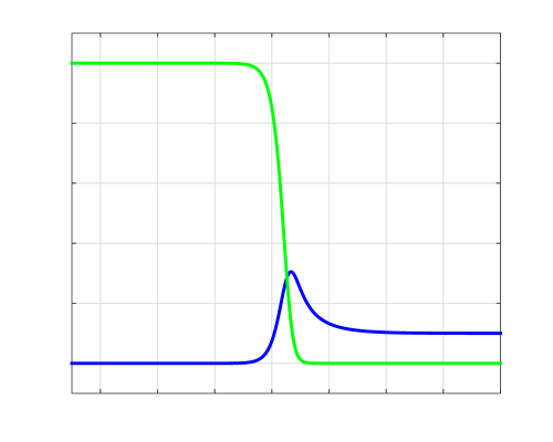
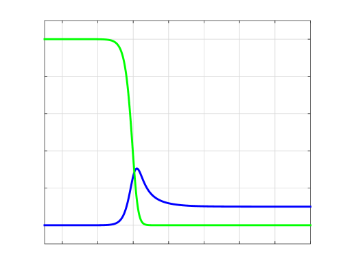
To begin with, we simulate the evolution in time of the population densities and .
The spatial domain is, as usual, approximated by a very large bounded domain with Neumann boundary conditions. Our initial condition is such that on the left and on the right.
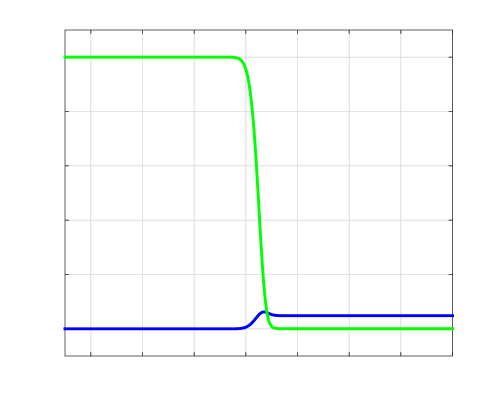
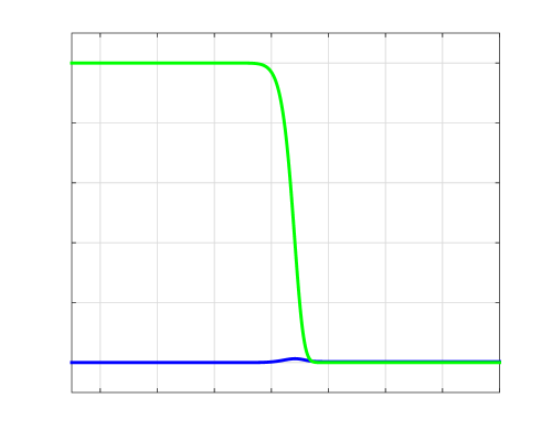
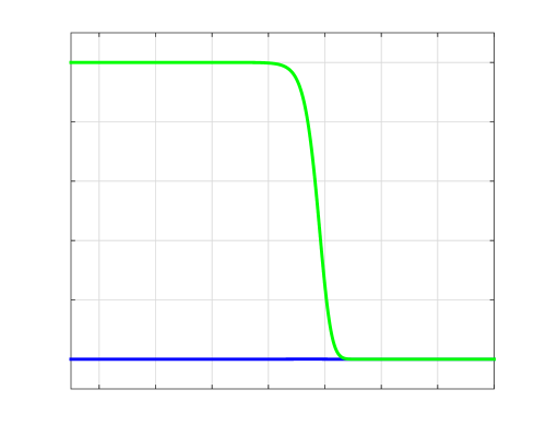
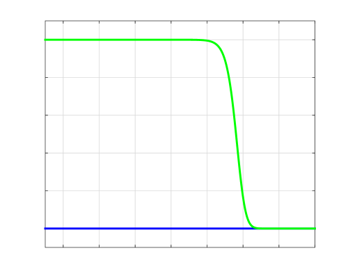
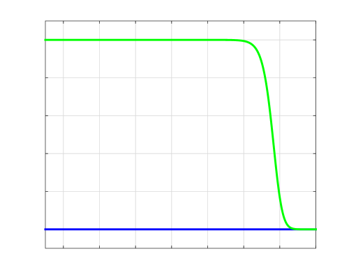
Time snapshots of such a simulation with and are presented in Figure 1. We clearly observe the rapid convergence of the solution to a traveling wave, namely to a solution with constant profile and constant wave speed . From now on, we use capital letters , , and for the wave profiles, functions of , and lower-case letters , , and for the population densities, functions of .
Note that by symmetry and isotropy, we would obtain an axis-symmetric figure if the gene drive was introduced on the left. If it was introduced in the center of a twice as large interval, we would observe the gluing of two traveling waves, one spreading towards the left at speed and the other spreading towards the right at speed .
With this choice of parameters and , we observe the so-called hair-trigger effect, namely the fact that no matter how small the height and the width of the initial , invasion occurs. This is a typical property of monostable dynamics, that fails with bistable dynamics. These lead on the contrary to what is referred to as threshold properties.
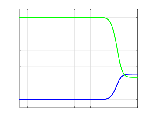
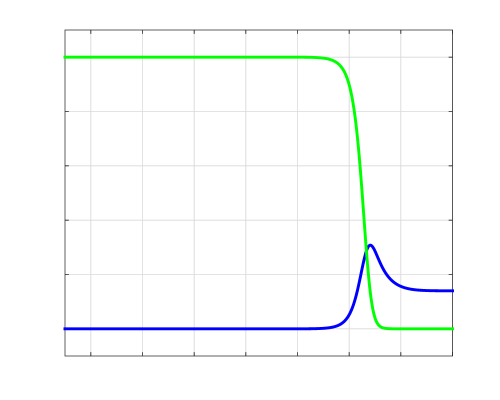
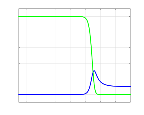


| ecological invasion |
| gene drive |
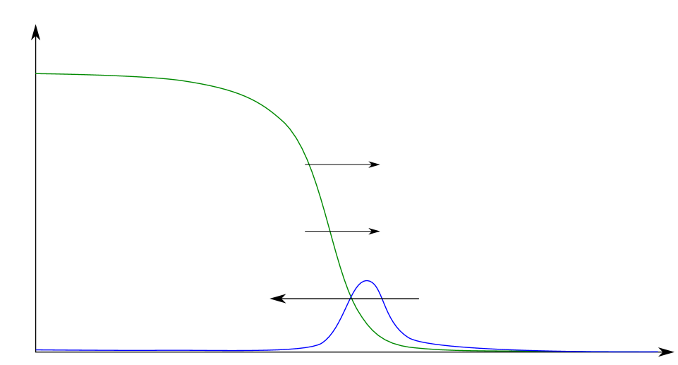
| natural selection |
Next, we let the parameters and vary. By doing so, we observe both a monostable regime, with hair-trigger effect, and a bistable regime, with threshold properties. In order to discard from our observations rapid extinctions of bistable gene drives due to an insufficiently large initial value of , in all following simulations we use as initial value on the right in a wide enough interval. With such a choice of initial data, we always observe on the right the convergence of to the steady state without wild-type .
We say that the gene drive invasion is successful, or that the gene drive is viable, if the invasion speed is negative. On the contrary, if , we say that the gene drive invasion fails and that the gene drive is nonviable: in particular, when , the gene drive is repelled and eliminated by the wild-type population. When introduced in the center of the spatial domain, a nonviable gene drive collapses in finite time.
In order to estimate the speed, it is convenient to have a well-defined level-set to follow. Hence we consider now the monotonicity of the traveling wave profiles. Although is in many cases not monotonic (see again Figure 1 and Figure 2), we observe in all simulated time evolutions the following monotonicities:
-
•
the wild-type population profile is strictly monotonic and connects to ;
-
•
the frequency profile (plots of not shown here) is monotonic – but not always strictly, as we sometimes observe everywhere;
-
•
the total population profile (plots of not shown here) is strictly monotonic and connects to .
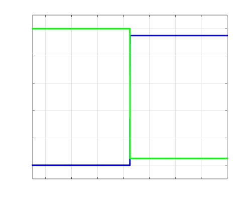
We systematically tested the above monotonicity properties of and in a wide parameter range for and . The result is displayed on Figure 3 and confirms the preceding claim – note that is negative as soon as and are respectively nonpositive and negative, whence it suffices to check the monotonicities of and . Therefore we can numerically estimate the speed by tracking the well-defined -level set of .

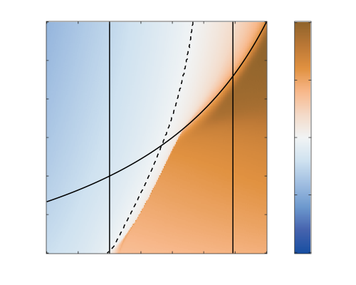
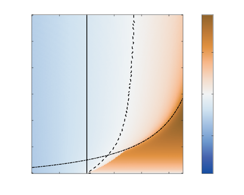
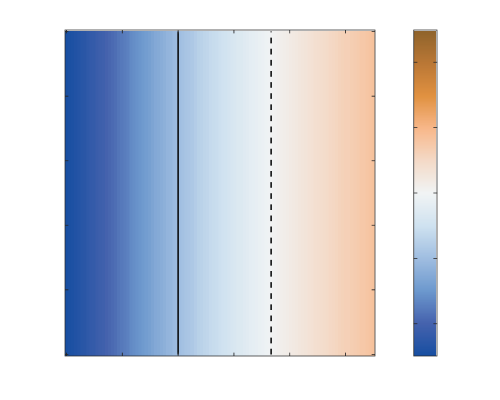
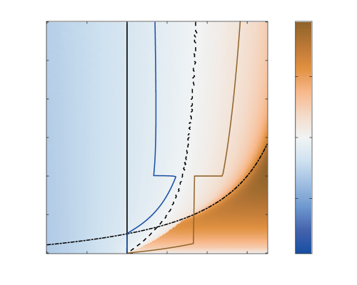
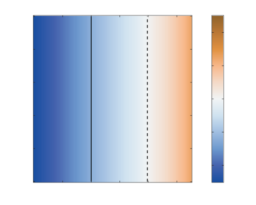
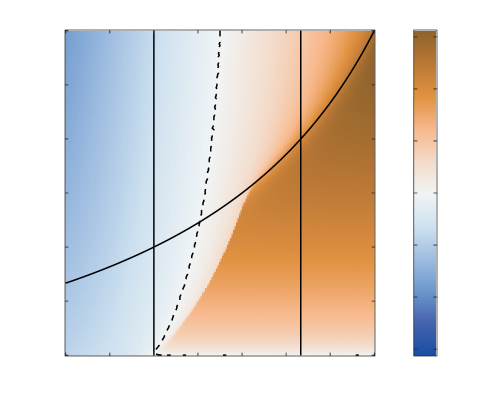
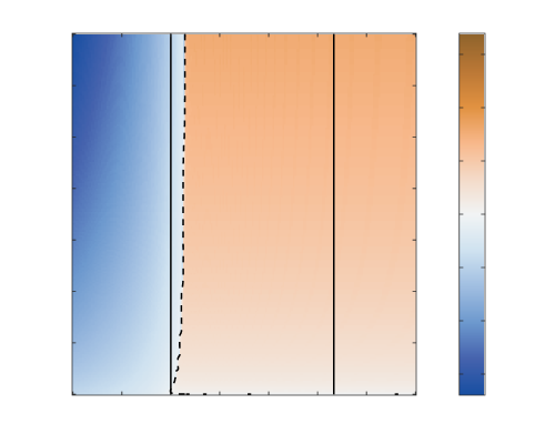
Estimations of the values of when and vary are displayed on heatmaps on Figure 4, where they are also compared to similar estimations for the density-independent equations (7) and (6) (both equations being in some way related to our model, cf. Section 1.5.1). Let us note that for the equation (7), whose reaction term is a classical cubic nonlinearity, an explicit formula is known for the bistable wave speed: . Hence its -level set is exactly at . For the more complicated equation (6) with a denominator, we do not know any algebraic formula for the wave speed but the -level set can still be computed approximately [36]: . Let us also point out that despite the fact that equation (7) arises as a weak selection approximation in Section 1.5.1, we plot its values for relatively large values of : in our opinion, it is interesting to compare on one hand the equation (6) and its weak selection approximation (7), as was done in Tanaka–Stone–Nelson [36], and on the other hand the equation (6) and our system (9). In particular, such a comparison clearly shows that accounting for population dynamics has a much stronger effect than accounting for strong selection.
The following comments on Figure 4(a) are in order.
-
•
The wave speed is (surprisingly to us) not a continuous function of . More precisely, a jump discontinuity divides into two parts the parameter region corresponding to nonviable eradication drives. Each part corresponds to a different kind of nonviable eradication drive: on the left-hand side of the discontinuity, we observe drives with strictly increasing (case of Figure 2), whereas on the right-hand side we observe drives with identically. For the latter kind, the traveling wave observed numerically (see Figure 5) is actually a classical Fisher–KPP traveling wave for the population: after having been eradicated from the right-hand side of the domain by the gene drive and having waited long enough for the eradication of the gene drive itself, the wild-type population invades the new open space at its Fisher–KPP speed . This is confirmed graphically by the fact that in the bottom right corner, the speed only depends on .
-
•
Away from this discontinuity, the -level set of seems to be an increasing, strictly convex curve, originating from and admitting a vertical straight line as asymptote. The equation of this asymptote has the form for some undetermined . In particular, the level set is included in : if , then and the gene drive invades; if , then and the gene drive is nonviable. These two conclusions for the parameter range were already valid for the density-independent equations (6) and (7) (see Figures 4(b) and 4(d)).
-
•
There exist viable eradication drives, yet the corresponding parameter region is small, especially when intersected with the half-space defined by .
1.6.2. Analytical results
Although finding the sign of the wave speed for a scalar bistable reaction–diffusion equation is easy (multiply the equation by the derivative of the wave profile and integrate over ), it is in general a very challenging problem for bistable reaction–diffusion systems of equations. The method used in the scalar case only works for systems whose reaction term has a specific gradient form – which is not the case here – and, apart from this method, no general method is known. Systems devoid of gradient form have to be studied on a case-by-case basis and most of the time these studies lead to results on very particular cases with specific algebraic requirements on the parameters of the system. For more details on this topic, we refer to the recent review by the first author on the sign of the wave speed for two-species Lotka–Volterra competition–diffusion systems [19].
Hence we believe that, given the present state of knowledge in the mathematical analysis of reaction–diffusion systems, an explicit complete characterization of the sign of is currently out of reach. We can nonetheless aim for a collection of partial results. In our opinion, the value of such results is twofold:
-
•
on one hand, they confirm in some regions of the parameter space the numerical experiments;
-
•
on the other hand, their proofs give precious insights on the deep structure of the equations, that might be useful in possible future work.
Regarding the existence of traveling waves with monotonic and , we point out first that the existence in the case identically reduces to a standard question for the Fisher-KPP equation and the conclusion is well known: there exists such a traveling wave with speed if and only if and the traveling wave with speed is unique (up to spatial translation). On the contrary, the case is a much more delicate issue here than in standard systems. On one hand, we will prove with Theorem 1.1 an explicit nonexistence result in a certain parameter range, showing that the existence for all values of is simply false. On the other hand, known methods for constructing traveling waves rely either on monotonicity properties of the reaction term and super-sub-solutions or on ODE shooting arguments with stable or unstable manifolds. Yet, both methods seem inappropriate here: both systems (9) and (10) have changing monotonicities and lack regularity as . We believe we might be able to obtain analytical existence results in certain parameter ranges (say, away from the eradication zone and for small values of where the system has a nice KPP structure [18]), but not in the range that interests us most, namely and in the eradication zone or close to it. Therefore we decide to leave the rigorous existence problem as an open problem444The empirical proof of existence provided by our numerical experiments might be sufficiently convincing for many non-mathematicians..
In any case, the biologically most relevant question is not the question of existence but rather the question of the direction of the propagation, namely the sign of the wave speed . Hence in the forthcoming Theorem 1.2 we will focus indeed on a priori estimates for this sign, or in other words we will study the sign of the wave speed of any existing traveling wave.
We use the variables to write the following theorems; the analogous results with variables can be written easily. In order to simplify the statements, we exclude traveling waves that are not monotonic or do not converge exponentially at ; this decision is consistent with numerical observations. We also choose to list only the results that give explicit regions of the plane where the sign is known, but our proofs actually give slightly larger implicit regions.
Definition 1.1.
A traveling wave solution of (10) is a bounded nonnegative classical solution of the form satisfying:
-
(1)
is nondecreasing, is decreasing;
-
(2)
.
Furthermore, the traveling wave is referred to as trivial if and nontrivial if .
Obviously, a trivial, respectively nontrivial, traveling wave solution of (9) is a solution such that the associated solution of (10) is a trivial, respectively nontrivial, traveling wave solution itself.
Our two main results follow. Graphically, they are summarized on Figure 4(c).
Theorem 1.1 (Nonexistence of nontrivial waves).
Consequently, for any traveling wave solution , is a Fisher–KPP traveling wave with speed .
Figure 5 is an example of spreading dynamics when and .
Theorem 1.2 (Sign of nontrivial wave speed).
Assume (10) admits a nontrivial traveling wave solution , in the sense of Definition 1.1, such that:
-
(1)
is strictly monotonic;
-
(2)
converges exponentially fast to at .
Then:
-
(1)
if:
-
(a)
; moreover, converges at to and ;
-
(b)
, , converges at to and
-
(c)
, , converges at to and
-
(a)
-
(2)
if:
-
(a)
and ;
-
(b)
and
-
(a)
2. Proof of Theorems 1.1 and 1.2
2.1. Proof of Theorem 1.1
Proposition 2.1.
Let be a solution of (9) set in with and for all and non-zero.
Then:
-
(1)
if , goes extinct spatially uniformly;
-
(2)
if and if is compactly supported, either does not spread or it spreads at most at speed .
Proof.
Using and then , we find that satisfies
By comparison principle, , where is the solution of the Fisher–KPP equation
If , the super-solution goes extinct uniformly, and so does . Otherwise, the asymptotic speed of spreading of the super-solution, which is an upper bound for the asymptotic speed of spreading of , is exactly the speed given in the statement. ∎
Corollary 2.2.
If , then all traveling waves are trivial.
Consequently, any wave speed satisfies .
2.2. Proof of Theorem 1.2
2.2.1. Viable gene drives
Proposition 2.3.
Assume (9) admits a nontrivial traveling wave solution satisfying
Then, if , necessarily .
Furthermore, if there exists such that
then implies .
Proof.
Close to , the wave profile is positive and, by virtue of the assumptions, increasing () and strictly convex (). Assuming by contradiction and plugging these inequalities into the traveling wave equation
we get
As the right-hand side converges to when , we deduce .
Subsequently, assuming the exponential convergence of with rate and passing to the limit into the equation, we discover
which has a positive solution if and only if . ∎
Proposition 2.4.
Assume (10) admits a nontrivial traveling wave solution with increasing .
Then, if , necessarily .
Proof.
First, we focus on the critical case .
By classification of the constant solutions of the system (10) when , necessarily such a traveling wave admits or as limit at . In all cases, converges to .
We use the strict monotonicity of and to establish the existence of
decreasing, bijective and of class , such that . Using a change of variable discovered by Nadin, Strugarek and Vauchelet [26], we deduce that there exists a traveling wave connecting to with increasing profile if and only if there exists a traveling wave solution of
where
with increasing profile as well. The reaction term is nonnegative and, by computing its derivatives at , it turns out that and : this equation is degenerate monostable. By standard results on degenerate monostable equations with non-degenerate second derivatives (prototypical reaction term ), there exists a traveling wave solution of speed for this equation if and only if , where .
Next, we consider the case . It is in fact proved similarly, except this time , so that we do not even need to look at . ∎
Proposition 2.5.
Assume (10) admits a nontrivial traveling wave solution with limit at and with increasing .
Then, if and if one of the following conditions holds true, necessarily :
-
(1)
-
(2)
Proof.
The case is already solved by the previous proposition, hence we assume without loss of generality . Moreover, the necessary nonnegativity of the limit implies ; the case of equality is discarded by assumption, so that we have .
Using again the relation and the change of variable of Nadin–Strugarek–Vauchelet [26], we find
Let be the integral in the right-hand side, so that . Using the strict positivity of , namely
we deduce
where . Consequently, if
that is if
This inequality is difficult to solve explicitly, however we point out that it is both true close to and false as .
The function
admits as derivative
which is negative in if and only if . Hence, in the particular case , the function is decreasing, so that the inequality can be improved as
which reduces to
This inequality can be rewritten as
This ends the proof. ∎
2.2.2. Nonviable gene drives
Previous propositions already confirm that nonviable gene drives can be found only in the parameter range .
When , the monotonicity of implies the convergence at to one constant solution among , (note that this value of is positive if and only if ) and .
The positivity of the speed being already established in the first case (trivial traveling waves), we focus on the second and third case (nontrivial traveling waves).
Proposition 2.6.
Let be a traveling wave solution of (10).
If one of the two following conditions holds true, the traveling wave is nontrivial and necessarily :
-
(1)
converges at to and ;
-
(2)
converges at to , and ;
-
(3)
is increasing, converges at to , and .
Proof.
Without loss of generality, assume .
First condition. The degenerate case is obvious ( is a standard Fisher–KPP traveling wave), whence we focus on .
Since , by comparison principle, and , where is the solution of
and is the asymptotic speed of spreading of . This spreading speed is larger than or equal to the associated minimal wave speed, which is positive.
Second condition. Since , by comparison principle, and , where is the solution of
and is the asymptotic speed of spreading of .
The spreading speed of such a bistable equation is exactly its unique traveling wave speed associated with an increasing profile having limits at and at .
Therefore the speed has the sign of the opposite of the integral over of
After some algebra we discover that
Hence if (and only if)
If , the positivity of yields a contradiction, so that is required additionally without loss of generality. Since implies , this ends the proof for the second condition.
Third condition. We use again the -diffeomorphism such that and the Nadin–Strugarek–Vauchelet formula [26]:
Recall that is decreasing in if . In such a case, it can be verified that the integral in the right-hand side above satisfies
where . Therefore, is positive if the latter integral is nonpositive, namely if . ∎
3. Discussion
3.1. Main conclusions
In [36], Tanaka et al. suggested the following terminology:
-
•
monostable gene drives, susceptible of hair-trigger effect, are socially irresponsible gene drives: the escape of just one individual carrying the gene drive allele from the laboratory suffices to trigger an invasion – they correspond to threshold-independent drives;
-
•
bistable gene drives, which can never invade if released accidentally in small quantities, are on the contrary socially responsible gene drives – they correspond to high-threshold drives.
This terminology can be combined with our viable/nonviable terminology: all socially irresponsible gene drives are viable but socially responsible gene drives can, stricto sensu, be viable or nonviable. Of course, practical gene drives should all be both viable and socially responsible. In Tanaka–Stone–Nelson’s density-independent model [36], this meant simply . However, in the model presented here, neither social responsibility (the drive is a threshold-dependent drive) nor viability (the drive is able to invade a wild-type population) can be easily and explicitly characterized with analytic methods. Numerical simulations become essential in understanding the interplay between the two parameters and .
Our model also shows that a gene drive can achieve complete eradication only if is small enough. This leads to a particulary striking conclusion: only very specific choices of and , corresponding to a small compact region in the -plane, can lead to socially responsible and viable eradication gene drives.
More generally, our model shows that the invasion of an eradication drive but also of any gene drive achieving only partial population suppression can be slowed down, stopped or even reversed by the opposing demographic advection term. Thus population dynamics matters for any gene drive affecting population size, even slightly, and should be taken into account. We however find that threshold-independent drives can spread spatially even when they lead to population suppression (thereby extending a result found by Beaghton et al. [5] for driving-Y to homing-based gene drives): their monostability property remains true, their hair-trigger effect is still observed numerically and the demographic advection term only slows them down but never stops them. For practical applications, this feature is especially dangerous if one thinks of threshold-independent eradication drives. These should definitely be approached with the highest caution.
Thus, ignoring population dynamics and only focusing on allele frequencies for spatial models of gene drive [36] should be limited to replacement drives, that correspond for instance to the weak selection framework (small values of ) or to very fast population dynamics (large values of ). We refer to the discussion in Section 1.5.1 on the relation between our model and the two density-independent equations (6) and (7).
3.2. Mathematical open problems worthy of attention
Characterizing analytically the asymptotics and , namely:
-
•
the transition at when , from nonexistent traveling waves to existent monostable traveling waves, without intermediate bistable regime;
-
•
the vertical asymptote of the level line , its precise value in and its relation with Strugarek–Vauchelet [35];
are two natural but difficult questions, that are left for further studies.
The main open problem with the systems (9) and (10) is the existence of nontrivial traveling waves. We briefly explained in Section 1.6.2 why this problem is very difficult: on one hand, the nonexistence result of Theorem 1.1 means that there will necessarily be requirements on the parameters and , and on the other hand known methods for proofs of existence are likely to be inappropriate, especially in the most interesting parameter range .
Some methods to construct traveling waves do not guarantee the monotonicity of the constructed profiles. Numerically, we only observed monotonic profiles and , but we did not manage to prove the a priori monotonicity of these profiles. Thus at this point it remains possible that traveling waves with non-monotonic profiles coexist with the observed monotonic ones.
These questions of existence lead to another related crucial issue: the stability properties of traveling waves555This whole paragraph is intentionally vague regarding the notion of stability, as we do not want to enter into details here. Of course, an unambiguous clarification would be necessary before any attempt at a rigorous proof.. Indeed, we know that trivial traveling waves always exist. When a trivial and a nontrivial wave coexist, can we predict theoretically which one is selected? The numerical experiments are ambivalent here. On one hand, they lead naturally to the following (rough) conjecture:
Conjecture 3.1.
In the whole parameter region where monotonic nontrivial traveling waves are numerically selected,
-
(1)
trivial traveling waves are unstable;
-
(2)
monotonic nontrivial traveling waves exist and are stable.
But on the other hand, it is numerically very challenging to distinguish cases where only trivial waves exist from cases where the two kinds coexist but the trivial ones are the only stable ones. Hence, at this point, it remains unclear whether the whole bottom right region of Figure 4(a) corresponds to a nonexistence result or not. We strongly believe that Theorem 1.1 is not optimal, but we do not know if we can expect the optimal result to cover the whole region where .
Finally, it would of course be interesting to improve our theoretical knowledge on the sign of the speed of nontrivial traveling waves. A direction that might be fruitful is the following: find upper or lower estimates for the decreasing function defined by and plug these estimates into the Nadin–Strugarek–Vauchelet formula [26] that we used repeatedly in the proofs:
Let us point out that a second similar formula can be obtained by integration by parts of the equation on multiplied by :
where . Unfortunately we did not manage to deduce anything interesting from this formula. But, again, it might prove fruitful once estimates on are established.
3.3. Effect of stochasticity
We checked the robustness of our results by running stochastic simulations of the model given in system (9). More precisely, our stochastic model is a variant of our deterministic model implemented as a modified Gillespie algorithm, with Brownian motion of individuals, numbers of offspring drawn according to a Poisson law and death times drawn according to an exponential law. Each simulation is stopped when one allele completely disappears from the spatial domain or when a given final time is reached (even if no allele has disappeared yet). Space was discretized into demes connected by dispersal to the nearest neighboring sites, with emigration probability equal to ; the carrying capacity of a deme is . The simulation codes are currently available online at https://plmlab.math.cnrs.fr/fdebarre/2021_DriveInSpace.
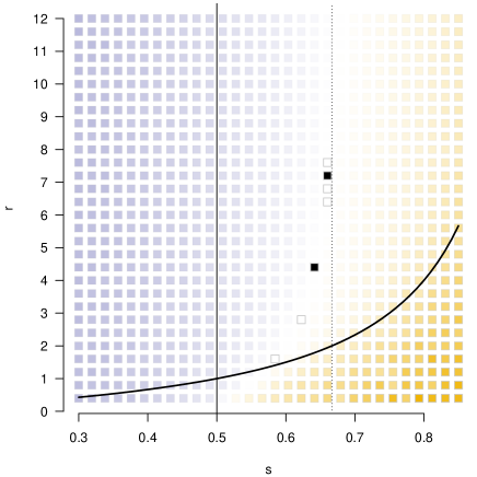
These simulations confirmed the results of the deterministic version of the model (compare Figure 6 to Figure 4(a)).
3.4. Genericity of this “wave reversal by opposing demographic advection” phenomenon
3.4.1. Other choices of birth and death rates
Numerically, several other cases were considered for and .
-
(1)
Constant death rate, weak or strong Allee effect on the wild-type dynamics with threshold : , (as a birth rate, has to be nonnegative). The Allee effect is weak if and strong if (if , there is again no Allee effect). The eradication condition is .
-
(2)
Constant birth rate, logistic wild-type growth: , . Again, the eradication condition is .
-
(3)
Constant birth rate, weak or strong Allee effect with threshold on the wild-type growth: , . The eradication conditions are or . Note that the first condition does not depend on .
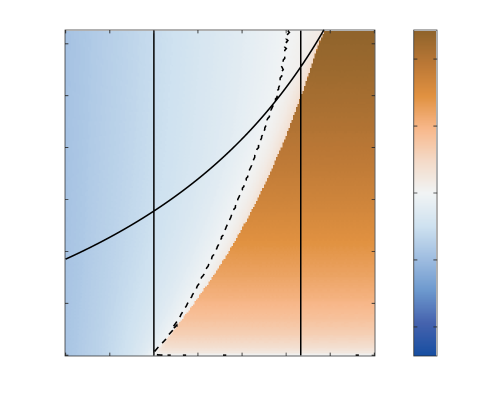
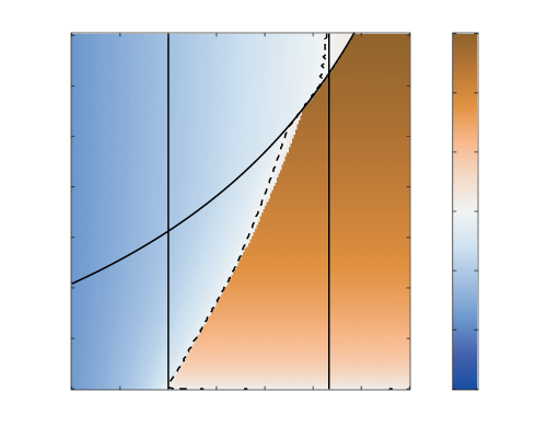
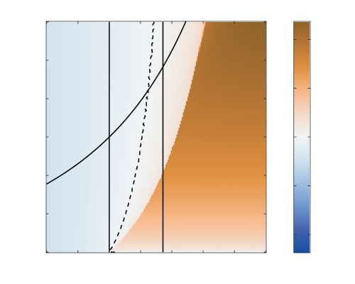
The resulting heatmaps can be observed on Figure 7. Interestingly, many features of Figure 4(a) remain true: the -level set is an increasing graph, it is stuck in the parameter range defined by the two thresholds and of the density-independent equation (7). However, the strong Allee effect on seems to break the strict convexity of the -level set and the strong Allee effect on seems to simply the picture in the sense that all nonviable gene drives satisfy .
We point out that many analytical techniques used in the proofs of Theorems 1.1 and 1.2 can be successfully applied to those cases. For the sake of brevity, we do not give details.
3.4.2. Other gene drive models
The same numerical method can be applied to different gene drive models: different particular cases of the system (1), particular cases of the analogous model obtained when assuming that the gene conversion (homing) occurs in the germline [31, 28], or entirely different models [36, 39, 11, 38]. We illustrate this possibility with two examples on Figure 8. Again, the main features of Figure 4(a) are preserved.
However we point out that our analytical tools strongly rely upon the fact that the system is a two-component system: most of them would be unapplicable in a three-component setting. This implies that models where three genotypes , and have to be tracked simultaneously cannot be studied this way. Our analytical approach seems to be limited to gene drives with perfect conversion and conversion in the zygote, for which heterozygous individuals can be safely ignored, or to models reduced by means of some approximation (e.g. Hardy-Weinberg proportions as in discrete-time models).
3.4.3. Extension to a bistable mosquito–Wolbachia model
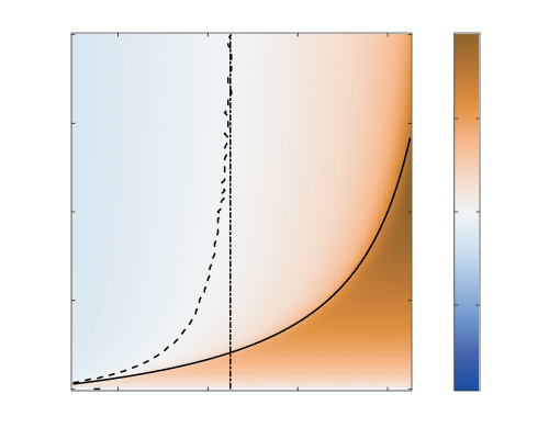
Finally, the same ideas can also be applied to different models from mathematical biology that share the common feature of leading to a two-component bistable reaction–diffusion system where one population with low carrying capacity tries to invade another population with high carrying capacity. Indeed, such a model will again involve an opposing advection term of the form and it should be clear at this point that this term is the main responsible for the qualitative features of Figure 4(a).
As an example, we consider a Wolbachia infection in a mosquito population, as described in [4, 34, 26]: the infection is transmitted vertically, perfectly, through mothers. The infection reduces fertility of mothers by a factor . Hatching rate is reduced by a factor for crosses involving an infected father and an uninfected mother. All other crossings have the same hatching rates. Assuming equal sex ratios, no sex differences in death rate and no differences in diffusion rate, we have
where and are the densities of infected and uninfected individuals, respectively, and is the total population density. Rewriting this system in terms of and , we obtain
The interior equilibrium for ,
| (11) |
is admissible (i.e., between and ) when ; it is unstable. With this example, we can indeed have a wave towards lower densities (a fully infected population is smaller than a fully uninfected population).
Numerical simulations for this model are displayed on Figure 9. Again, this figure shares many similarities with Figure 4(a). This illustrates once more that the important term in this whole class of models when concerned about spreading properties is the opposing advection term.
3.5. Biological implications
We found that a threshold-independent homing drive would spread spatially, even if it leads to the eradication of the target population. This extends the results of Beaghton et al. [5], obtained by a driving-Y, to another type of gene drive. For threshold-dependent drives, however, we find that the parameter space allowing for spatial spread is more restricted than what is found in models neglecting changes in population size and the resulting opposing demographic advection of individuals [36]. These simpler models find that a drive spreads as long as the release threshold is sufficiently low (lower than in [3, 4], lower than a value close to in [36]) and the initial condition is sufficiently large. In contrast, we find that these conclusions remain true for pure replacement drives but that spatial spread is limited for suppression or eradication drives, all the more as suppression is strong. These conclusions can be extended to other, non-drive, systems for population control such as Wolbachia.
The parameter range displayed on Figure 4 and other figures for the Malthusian growth rate, namely , seems to be biologically realistic and relevant. Indeed, we found in [41] for Aedes aegypti, in [13] for Aedes aegypti, in [25] for Anopheles gambiae, in [22] for Anopheles stephensi 666From [41, 13, 25, 22], is deduced by using the formula , where is the constant adult reproduction rate (namely, the birth rate corrected by taking into account juvenile mortality), is the constant adult death rate, and and are given in the same unit, say day-1. Compared with the classical formula , here we divide by to account for the fact that in system (9) the time unit is modified so that the death rate is scaled to ., in [32] for Aedes albopictus.
We have hence characterised a new reason for the failure of spatial spread of suppression drives, in the form of opposing demographic advection. This phenomenon was expected given previous work on spatial dynamics of alleles (as reviewed in [12]), but we clarify conditions under which it occurs. Other models of spatial spread, and in particular individual-based models, had already identified some reasons why the spatial spread of a suppression drive may fail. If the drive suppresses the local population too much and if the density target population is spatially heterogeneous, the drive may go extinct locally with the eradication of a local subpopulation before it could spread to other locations [29]. Strategies relying on the eradication of the target population are also limited by the potential recolonization of emptied locations by wild-type individuals [29, 30, 9] (such recolonizations can also be observed in our stochastic simulations). Finally, the evolution of resistance to the drive itself, which already hinders the success of gene drives in well-mixed populations [37], also affects their spatial spread [6].
Our model was derived under limiting assumptions, including a homing rate, and either homing taking place very early in development or the drive being dominant. Gene drives currently being designed in laboratories do not exactly match these assumptions. While we are pessimistic that analytical results can be obtained when these assumptions are relaxed, future numerical or computational (individual-based) studies will be useful to assess the generality of our findings. The results of individual-based simulations of the spatial spread of underdominance gene drive systems [10] are encouraging. The authors indeed found limited spatial spread even in the case of , in simulations initiated with the left half of the arena occupied by drive homozygotes and the right half by wild-type homozygotes (2L2T system; Fig. 3F) – initial conditions similar to ours.
To conclude, this work highlights the importance of not neglecting demographic dynamics in evolutionary models when the spread of an allele affect the size of a population.
Acknowledgements
We are grateful to the INRAE MIGALE bioinformatics facility (MIGALE, INRAE, 2020. Migale bioinformatics Facility, doi: 10.15454/1.5572390655343293E12) for providing computing resources. FD is funded by an Agence Nationale de la Recherche JCJC grant TheoGeneDrive ANR-19-CE45-0009-01.
References
- [1] Luke S. Alphey, Andrea Crisanti, Filippo (Fil) Randazzo, and Omar S. Akbari. Opinion: Standardizing the definition of gene drive. Proceedings of the National Academy of Sciences, 117(49):30864–30867, December 2020.
- [2] Philipp M. Altrock, Arne Traulsen, R. Guy Reeves, and Floyd A. Reed. Using underdominance to bi-stably transform local populations. Journal of Theoretical Biology, 267(1):62–75, November 2010.
- [3] N H Barton. The dynamics of hybrid zones. Heredity, 43(3):341–359, December 1979.
- [4] Nick H. Barton and Michael Turelli. Spatial waves of advance with bistable dynamics: Cytoplasmic and genetic analogues of Allee effects. The American Naturalist, 178(3):E48–E75, 2011. PMID: 21828986.
- [5] Andrea Beaghton, Pantelis John Beaghton, and Austin Burt. Gene drive through a landscape: Reaction–diffusion models of population suppression and elimination by a sex ratio distorter. Theoretical Population Biology, 108:51–69, April 2016.
- [6] Andrea Beaghton, Andrew Hammond, Tony Nolan, Andrea Crisanti, H. Charles J. Godfray, and Austin Burt. Requirements for Driving Antipathogen Effector Genes into Populations of Disease Vectors by Homing. Genetics, 205(4):1587–1596, April 2017.
- [7] Austin Burt. Site-specific selfish genes as tools for the control and genetic engineering of natural populations. Proceedings of the Royal Society of London. Series B: Biological Sciences, 270(1518):921–928, May 2003.
- [8] Jackson Champer, Anna Buchman, and Omar S. Akbari. Cheating evolution: engineering gene drives to manipulate the fate of wild populations. Nature Reviews Genetics, 17(3):146–159, March 2016.
- [9] Jackson Champer, Isabel Kim, Samuel E. Champer, Andrew G. Clark, and Philipp W. Messer. Suppression gene drive in continuous space can result in unstable persistence of both drive and wild-type alleles. preprint, Ecology, September 2019.
- [10] Jackson Champer, Joanna Zhao, Samuel E. Champer, Jingxian Liu, and Philipp W. Messer. Population Dynamics of Underdominance Gene Drive Systems in Continuous Space. ACS Synthetic Biology, 9(4):779–792, April 2020.
- [11] Anne Deredec, Austin Burt, and H. C. J. Godfray. The population genetics of using homing endonuclease genes in vector and pest management. Genetics, 179(4):2013–2026, 2008.
- [12] Sumit Dhole, Alun L Lloyd, and Fred Gould. Gene drive dynamics in natural populations: The importance of density dependence, space and sex. Annual review of ecology, evolution, and systematics, 51(1):505–531, November 2020.
- [13] Christopher Dye. Models for the population dynamics of the yellow fever mosquito, Aedes aegypti. Journal of Animal Ecology, 53(1):247–268, 1984.
- [14] John W. Eaton, David Bateman, Søren Hauberg, and Rik Wehbring. GNU Octave version 5.1.0 manual: a high-level interactive language for numerical computations, 2019.
- [15] EFSA Panel on Genetically Modified Organisms (GMO), Hanspeter Naegeli, Jean‐Louis Bresson, Tamas Dalmay, Ian C Dewhurst, Michelle M Epstein, Philippe Guerche, Jan Hejatko, Francisco J Moreno, Ewen Mullins, Fabien Nogué, Nils Rostoks, Jose J Sánchez Serrano, Giovanni Savoini, Eve Veromann, Fabio Veronesi, Michael B Bonsall, John Mumford, Ernst A Wimmer, Yann Devos, Konstantinos Paraskevopoulos, and Leslie G Firbank. Adequacy and sufficiency evaluation of existing EFSA guidelines for the molecular characterisation, environmental risk assessment and post‐market environmental monitoring of genetically modified insects containing engineered gene drives. EFSA Journal, 18(11), November 2020.
- [16] Kevin M. Esvelt, Andrea L. Smidler, Flaminia Catteruccia, and George M. Church. Emerging Technology: Concerning RNA-guided gene drives for the alteration of wild populations. eLife, 3:e03401, jul 2014.
- [17] Ronald Aylmer Fisher. The wave of advance of advantageous genes. Annals of eugenics, 7(4):355–369, 1937.
- [18] Léo Girardin. Non-cooperative Fisher–KPP systems: traveling waves and long-time behavior. Nonlinearity, 31(1):108, 2018.
- [19] Léo Girardin. The effect of random dispersal on competitive exclusion – A review. Math. Biosci., 318:108271, 2019.
- [20] Léo Girardin, Vincent Calvez, and Florence Débarre. Catch me if you can: A spatial model for a brake-driven gene drive reversal. Bulletin of Mathematical Biology, 81(12):5054–5088, Dec 2019.
- [21] Gili Greenbaum, Marcus W. Feldman, Noah A. Rosenberg, and Jaehee Kim. Designing gene drives to limit spillover to non-target populations. preprint, Evolutionary Biology, June 2019.
- [22] Nadira Haq, William K. Reisen, and Muhammad Aslamkhan. The effects of Nosema algerae on the horizontal life table attributes of Anopheles stephensi under laboratory conditions. Journal of Invertebrate Pathology, 37(3):236 – 242, 1981.
- [23] Andrei N. Kolmogorov, I. G. Petrovsky, and N. S. Piskunov. Étude de l’équation de la diffusion avec croissance de la quantité de matière et son application à un problème biologique. Bulletin Université d’État à Moscou, 1:1–25, 1937.
- [24] John M. Marshall and Bruce A. Hay. Confinement of gene drive systems to local populations: A comparative analysis. Journal of Theoretical Biology, 294:153–171, February 2012.
- [25] P. O. Mireji, J. Keating, A. Hassanali, C. M. Mbogo, M. N. Muturi, J. I. Githure, and J. C. Beier. Biological cost of tolerance to heavy metals in the mosquito Anopheles gambiae. Medical and Veterinary Entomology, 24(2):101–107, 2010.
- [26] Grégoire Nadin, Martin Strugarek, and Nicolas Vauchelet. Hindrances to bistable front propagation: application to Wolbachia invasion. J. Math. Biol., 76(6):1489–1533, 2018.
- [27] Engineering National Academies of Sciences and Medicine. Gene Drives on the Horizon: Advancing Science, Navigating Uncertainty, and Aligning Research with Public Values. The National Academies Press, Washington, DC, 2016.
- [28] Charleston Noble, Jason Olejarz, Kevin M. Esvelt, George M. Church, and Martin A. Nowak. Evolutionary dynamics of CRISPR gene drives. Science Advances, 3(4):e1601964, April 2017.
- [29] Ace North, Austin Burt, and H. Charles J. Godfray. Modelling the spatial spread of a homing endonuclease gene in a mosquito population. Journal of Applied Ecology, 50(5):1216–1225, October 2013.
- [30] Ace R. North, Austin Burt, and H. Charles J. Godfray. Modelling the potential of genetic control of malaria mosquitoes at national scale. BMC Biology, 17(1):26, December 2019.
- [31] Nicolas O. Rode, Virginie Courtier-Orgogozo, and Florence Débarre. Can a population targeted by a CRISPR-based homing gene drive be rescued? G3: Genes, Genomes, Genetics, 10(9):3403–3415, 2020.
- [32] Lionel Roques and Olivier Bonnefon. Modelling population dynamics in realistic landscapes with linear elements: A mechanistic-statistical reaction-diffusion approach. PLOS ONE, 11(3):1–20, 03 2016.
- [33] Steven P. Sinkins and Fred Gould. Gene drive systems for insect disease vectors. Nature Reviews Genetics, 7(6):427–435, June 2006.
- [34] Martin Strugarek. Mathematical modeling of population dynamics, applications to vector control of Aedes spp. (Diptera:Culicidae). Theses, Sorbonne Université , UPMC, September 2018.
- [35] Martin Strugarek and Nicolas Vauchelet. Reduction to a single closed equation for 2-by-2 reaction-diffusion systems of Lotka-Volterra type. SIAM J. Appl. Math., 76(5):2060–2080, 2016.
- [36] Hidenori Tanaka, Howard A. Stone, and David R. Nelson. Spatial gene drives and pushed genetic waves. Proceedings of the National Academy of Sciences, 114(32):8452–8457, 2017.
- [37] Robert L. Unckless, Andrew G. Clark, and Philipp W. Messer. Evolution of resistance against crispr/cas9 gene drive. Genetics, 205(2):827–841, 2017.
- [38] Robert L. Unckless, Philipp W. Messer, Tim Connallon, and Andrew G. Clark. Modeling the manipulation of natural populations by the mutagenic chain reaction. Genetics, 201(2):425–431, 2015.
- [39] Michael R. Vella, Christian E. Gunning, Alun L. Lloyd, and Fred Gould. Evaluating strategies for reversing CRISPR-Cas9 gene drives. Scientific Reports, 7(1):11038, 2017.
- [40] J. H. Werren. Selfish genetic elements, genetic conflict, and evolutionary innovation. Proceedings of the National Academy of Sciences, 108(Supplement_2):10863–10870, June 2011.
- [41] Steven M. White, Pejman Rohani, and Steven M. Sait. Modelling pulsed releases for sterile insect techniques: fitness costs of sterile and transgenic males and the effects on mosquito dynamics. Journal of Applied Ecology, 47(6):1329–1339, 2010.
