Investment vs. reward in a competitive knapsack problem

Abstract

Natural selection drives species to develop brains, with sizes that increase with the complexity of the tasks to be tackled. Our goal is to investigate the balance between the metabolic costs of larger brains compared to the advantage they provide in solving general and combinatorial problems. Defining advantage as the performance relative to competitors, a two-player game based on the knapsack problem is used. Within this framework, two opponents compete over shared resources, with the goal of collecting more resources than the opponent. Neural nets of varying sizes are trained using a variant of the AlphaGo Zero algorithm [1]. A surprisingly simple relation, $N_{A}/(N_{A}+N_{B})$, is found for the relative win rate of a net with $N_{A}$ neurons against one with $N_{B}$. Success increases linearly with investments in additional resources when the networks sizes are very different, i.e. when $N_{A}\ll N_{B}$, with returns diminishing when both networks become comparable in size.

1 Introduction

Optimal resource allocation often leads to combinatorial problems, e.g. time can be minimized by solving the travelling salesman problem. In nature, resource allocation is in many cases a competitive process, with animals competing with each other over shared resources. A key question regards in this context the balance between success rate and investments in computational capabilities, e.g. in terms of metabolic cost. This question is relevant also for artificial neural networks, which are notoriously bad at solving combinatorial problems [2], in particular when compared with the performance of traditional, problem-specific algorithms.

Lately, there has been a rising interest to apply deep learning architectures to combinatorial problems [3] [4] [5]. In this context we are interested in the evolutionary factors determining network sizes, when assuming that larger nets come with correspondingly larger metabolic cost. Presently it is however unclear how costs scale with reward, that is the precise functional dependence of success on network size is not known. Here we investigate this question within the 0-1 knapsack problem, a basic resource allocation task that can be generalize to a range of real-world situations [6].

The problem is defined as follows: Given $n$ items with values $v_{i}$ and weights $w_{i}$, maximize

$$\sum_{i=1}^{n}{v_{i}x_{i}},\quad\quad x_{i}\in\{0,1\}\,,$$ (1)

subject to a capacity constraint

$$\sum_{i=1}^{n}{w_{i}x_{i}}\,\leq\,W\,,$$ (2)

where $\{x_{i}\}$ denotes the chosen subset of items and $W$ is a constraint on the total weight. In other words, one should select the group of items with maximal total value which does not exceed the total weight limit. There are several algorithms developed specifically to solve the 0-1 knapsack problem and special cases of it, such as dynamic programming and branch-and-bound algorithms [7].

Survival of the fittest pushes species to become better than their competition, when too many individuals are fighting for the same resources. It is therefore logical to measure the success of an agent only in comparison to other agents, rather than looking for an absolute scale. For this reason we decided to focus on a two-player extension of the knapsack problem. In this setup, two agents compete over the same pool of resources trying each to collect more value than the other. This framework allowed us to use a powerful tool for training deep learning models to play turn based games, the AlphaGo Zero ($\alpha$GZ) algorithm [1]. Suitably adapted, we applied $\alpha$GZ to train neural network models of varying sizes $N$ to play the two-player knapsack game, with the goal of comparing their performances when playing against each other. This framework allows us to determine how increasing the number of available neurons affects the performance of the competing networks.

2 Method

In order to simulate direct interactions between agents, we created a zero sum game for two players which is an extension of the knapsack problem. During the course of a game, players pick items in turns from a common item pool. Each item can be selected by at most one player, and each player has a capacity limit for the total weight of items they can personally collect. The goal of the game is not to maximize the total value of items collected, but rather to surpass the total value gained by the opponent. A game progresses in the following manner:

• Each turn, a player may choose any item from the pool of free items and add it to their collection, provided this would not cause the total weight of items collected to exceed the weight limit. The item chosen is then removed from the common pool, and the other player plays his turn. If no suitable item is available, the current player passes.

• The two players take their turns one after the other, until no item is picked for two consecutive turns, meaning there are no more valid items. At this point the player with the larger total value is declared the winner.

For our simulations we focused on games where items are unique, $v_{i}\neq v_{j}$ for $i\neq j$, with both players having identical capacity limits. Since generating $v_{i},w_{i}$ from a uniform distribution creates mostly easily solvable knapsack problem instances [8], we generated weakly correlated instances [9], which are generally harder to solve. These are defined as instances where $w_{i}$ is uniformly distributed in $[0,1]$ and $v_{i}$ is uniformly distributed in a range of $w_{i}\pm 0.1$, confined to $[0,1]$. The capacity limits were set to $W=n/4$ as this avoids generating easy instances in the normal knapsack problem setting [10]. The complexity of the two player framework is somewhat increased, as compared to the original knapsack problem, as players need to deprive the opponent of items, in addition to optimizing their own collection.

Training was done using an adaptation of the $\alpha$GZ algorithm. The neural network agents are trained by reinforcement learning on self generated data, without using any a priori knowledge of the game. The networks receive as inputs the current state of the game, i.e. the weights and values of all items and a list of all items acquired so far by each player. The output consists of a policy vector and a value prediction:

$$f(s)=(\vec{p},v)\,,$$ (3)

where $v$ is a prediction of the value of the current game position $s$, which is equivalent to the expected final outcome of the game from this position. We set the possible game outcomes to be $\{0,1\}$, for losing/winning the game respectively, therefore implying that $v\in[0,1]$. $\vec{p}$ is a probability distribution over all available moves, which should prioritize better moves and is used to guide the Monte Carlo tree search (MCTS). The neural net is trained on randomly picked game states that were visited in previous games played, using the loss function:

$$l=(z-v)^{2}-\vec{\pi}\log\vec{p}\,.$$ (4)

Here $z$ is the recorded game outcome and $\vec{\pi}$ is an improved policy vector generated by the MCTS. Before each training phase, several games are played using the current version of the agent, pitched against a copy of itself. During a game, each player makes use of a search tree in order to choose every move. The tree contains a parent node holding information about the current game state, with nodes descending from it for each possible future game state that has been explored before. Every turn, the agent is given a certain number of iterations to expand their search tree, before deciding which move to make.

MCTS makes use of the information stored in each node in order to expand new leaf nodes. A node contains four parameters: The number of times the node has been visited in previous searches, $N$; the sum of all scores predicted for this node and its children, $W$; the mean score $Q={W}/{N}$; and the policy vector $\vec{p}$ calculated once by the agent for this game state. Each iteration of expanding the tree traverses it by starting at the first node, i.e. the current game state, and repeatedly moving to the child node which maximizes a quantity $Q+U$ until a previously unvisited node is reached. The term $U$ is defined according to:

$$U=cP_{a}\frac{\sqrt{\sum_{i}N_{i}}}{1+N_{a}}\,,$$ (5)

where $c$ is a constant, $P_{a}$ is the policy vector element corresponding to action $a$ leading to the node, $N_{a}$ is the node’s visit count and $\sum_{i}N_{i}$ is the sum of the visit counts of all available actions. When an unexplored node is reached, it is added to the tree and the parameters of it and all other nodes traversed are updated. After the expansion iterations are done a move is chosen according to an improved policy $\vec{\pi}$, defined by using the visit counts of all possible moves:

$$\pi_{i}\propto N_{i}^{1/\tau}$$ (6)

With $\tau$ a temperature parameter controlling the degree of exploration, set to $1$ in our case. The turn then ends, and both players trim their search trees to remove all nodes that are now unreachable, making the new game state the parent node of the whole tree.

We trained fully connected feed forward neural network models to play two-player knapsack games with 16 items. Each net had 2 hidden layers with ReLU connections, both with the same number of neurons, which changed from one net to the other. The inputs consisted of 4 vectors of length 16: A vector of the items’ weights, a vector of the values and two binary vectors encoding the items taken by each player. The items were ordered by descending ratio of $v_{i}/w_{i}$ such that a minimal sized model could easily implement a greedy strategy of picking the items with the best ratios. The network outputs were a policy vector with a softmax activation and a value head with a sigmoid activation. Every net was trained on a total of 40,000 self generated games, where optimization steps were taken every 40 games and performance was evaluated every 4,000 games, saving the best performing version. Each evaluation step consisted of 200 games of the net against a greedy algorithm in order to save time. The agents used 40 Monte Carlo steps per turn in all games. All model instances were given the same number of optimization steps regardless of their sizes, without early stopping if performance saturated. The final results presented in the next section were generated by training four separate copies of each net and taking the average of their game outcomes.

In order to interpret our results we made use of the Elo rating system [11], a rating system for zero-sum games that was invented for chess and gained popularity in numerous games. The expected score, or winning probability, of player $A$ over player $B$ is given by the formula:

$$P_{A}=\frac{1}{1+10^{(R_{B}-R_{A})/400}}\,,$$ (7)

where $R_{A},R_{B}$ are the Elo ratings of both players. These ratings are found by repeatedly matching players together and adjusting their ratings to fit the game outcomes.

3 Results and discussion

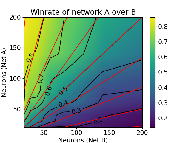
(a)

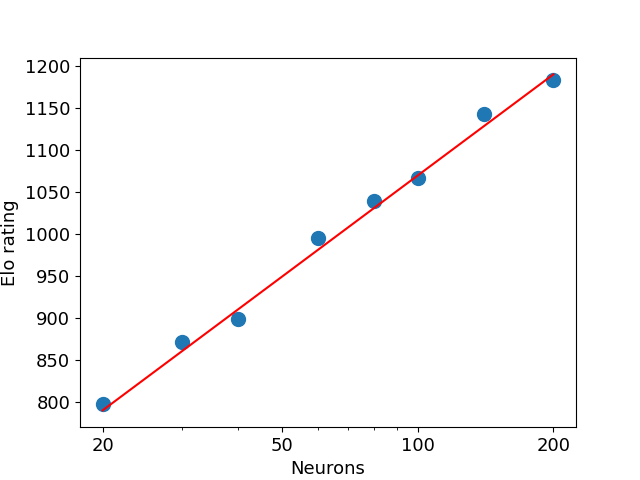
(b)

Figure 1: Training neural networks to play competitive knapsack problem games with 16 items. (a) Probability of net A to win against net B, when both have differing numbers of neurons. The black lines mark increments of 0.1 in winning probability, the red lines mark the same for the prediction given by Eq. ( 8). (b) Elo rating of networks with different numbers of neurons in log scale, with the logarithmic fit $y=400\log(N)+const$ in red.

Combinatorial problems manifest themselves in many ways in nature, making it beneficial for organisms to evolve ways to solve them. But unlike raw mathematical problems which have in most cases goals and solving conditions that are defined in absolute terms, in the natural world evolution pushes agents to overcome their competition such that merit is measured predominantly in relation to one’s competitors. It is therefore biologically sensible to look at adversarial problems when analysing the performance of neural networks at solving combinatorial problems. This is why we chose to work on the two-player competitive version of the knapsack problem, where the merit of an agent in relation to other agents is clearly defined by the probability of winning or losing a game against them. Figure 1 presents the outcome of training neural nets of varying sizes to play a competitive knapsack problem game with 16 weakly correlated items [9]. All neural nets contained two hidden layers, both with the same number of neurons, which was changed from one net to the other.

The problem displays diminishing returns, requiring increasingly larger differences between the sizes of competing nets in order to maintain the same win-lose statistics between them as they increase in size. This is supported by plotting the Elo rating of the nets, which scales logarithmically in network size. In fact the Elo rating is fitted well by $y=400\log(N)+const$, where $N$ is the number of hidden neurons. Since $400$ is the Elo scaling factor, plugging this expression into Eq. (7) reveals that the probability of net A to win a game against net B reduces to

$$P_{A}=\frac{N_{A}}{N_{A}+N_{B}}\,,$$ (8)

where $N_{A},N_{B}$ are the numbers of hidden neurons of nets A and B respectively. In other words, the probability of player A to win is $N_{A}/N_{B}$ times greater than that of player B, meaning the performance of neural nets against each other in this task is determined directly by the ratio of their sizes.

A peculiar property of the Elo rating system is that it assumes the existence of an absolute rating scale which determines game outcomes solely according to the difference in ratings between the two players. It could be possible that other factors also affect game outcomes, which would require a more complex model. To rule out this possibility, we plotted the full map of game outcomes for every combination of players in Figure 1(a). Lines of equal winning probability predicted by Eq. (8) are marked in red. It is clear that the theoretical prediction matches the corresponding lines obtained through simulations (in black) to an astonishing degree, proving that Eq. (8) holds.

This result implies a linear increase of the probability $P_{A}$ with network size in the regime where $N_{A}\ll N_{B}$, and diminishing returns when both opponents are relatively equally matched. Therefore a large difference between competitors can be quickly closed when they evolve to maximize their own utility. Note that when $N_{A}\approx N_{B}$ the benefit of increasing the number of neurons by a multiplicative factor, $N_{A}\to\gamma N_{A}$, is independent of $N_{A}$, always yielding the same winning probability ${\gamma}/(\gamma+1)$.

References

- [1] David Silver, Julian Schrittwieser, Karen Simonyan, Ioannis Antonoglou, Aja Huang, Arthur Guez, Thomas Hubert, Lucas Baker, Matthew Lai, Adrian Bolton, et al. Mastering the game of go without human knowledge. nature, 550(7676):354–359, 2017.
- [2] Kate A Smith. Neural networks for combinatorial optimization: a review of more than a decade of research. INFORMS Journal on Computing, 11(1):15–34, 1999.
- [3] Kenshin Abe, Zijian Xu, Issei Sato, and Masashi Sugiyama. Solving np-hard problems on graphs with extended alphago zero. arXiv preprint arXiv:1905.11623, 2019.
- [4] Elias Khalil, Hanjun Dai, Yuyu Zhang, Bistra Dilkina, and Le Song. Learning combinatorial optimization algorithms over graphs. In Advances in Neural Information Processing Systems, pages 6348–6358, 2017.
- [5] Irwan Bello, Hieu Pham, Quoc V Le, Mohammad Norouzi, and Samy Bengio. Neural combinatorial optimization with reinforcement learning. arXiv preprint arXiv:1611.09940, 2016.
- [6] Carsten Murawski and Peter Bossaerts. How humans solve complex problems: The case of the knapsack problem. Scientific reports, 6:34851, 2016.
- [7] Silvano Martello, David Pisinger, and Paolo Toth. New trends in exact algorithms for the 0–1 knapsack problem. European Journal of Operational Research, 123(2):325–332, 2000.
- [8] Kate Smith-Miles and Leo Lopes. Measuring instance difficulty for combinatorial optimization problems. Computers & Operations Research, 39(5):875–889, 2012.
- [9] David Pisinger. Where are the hard knapsack problems? Computers & Operations Research, 32(9):2271–2284, 2005.
- [10] Mattias Ohlsson, Carsten Peterson, and Bo Söderberg. Neural networks for optimization problems with inequality constraints: the knapsack problem. neural computation, 5(2):331–339, 1993.
- [11] Mark E Glickman and Albyn C Jones. Rating the chess rating system. CHANCE-BERLIN THEN NEW YORK-, 12:21–28, 1999.