Sampling a Near Neighbor in High Dimensions

Abstract.

Similarity search is a fundamental algorithmic primitive, widely used in many computer science disciplines. Given a set of points $S$ and a radius parameter $r>0$, the $r$-near neighbor ($r$-NN) problem asks for a data structure that, given any query point $q$, returns a point $p$ within distance at most $r$ from $q$. In this paper, we study the $r$-NN problem in the light of individual fairness and providing equal opportunities: all points that are within distance $r$ from the query should have the same probability to be returned. In the low-dimensional case, this problem was first studied by Hu, Qiao, and Tao (PODS 2014). Locality sensitive hashing (LSH), the theoretically strongest approach to similarity search in high dimensions, does not provide such a fairness guarantee.

In this work, we show that LSH based algorithms can be made fair, without a significant loss in efficiency. We propose several efficient data structures for the exact and approximate variants of the fair NN problem. Our approach works more generally for sampling uniformly from a sub-collection of sets of a given collection and can be used in a few other applications. We also develop a data structure for fair similarity search under inner product that requires nearly-linear space and exploits locality sensitive filters. The paper concludes with an experimental evaluation that highlights the inherent unfairness of NN data structures and shows the performance of our algorithms on real-world datasets.

Preliminary versions of the results of this paper were published in (Har-Peled and Mahabadi, 2019; Aumüller et al., 2020b).

1. Introduction

In recent years, following a growing concern about the fairness of the algorithms and their bias toward a specific population or feature (Hardt et al., 2016; Chouldechova, 2017; Munoz et al., 2016; Kleinberg et al., 2017), there has been an increasing interest in building algorithms that achieve (appropriately defined) fairness (Dwork et al., 2012). The goal is to remove, or at least minimize, unethical behavior such as discrimination and bias in algorithmic decision making, as nowadays, many important decisions, such as college admissions, offering home loans, or estimating the likelihood of recidivism, rely on machine learning algorithms. While algorithms are not inherently biased, nevertheless, they may amplify the already existing biases in the data. Hence, this concern has led to the design of fair algorithms for many different applications, e.g., (Donini et al., 2018; Agarwal et al., 2018; Pleiss et al., 2017; Chierichetti et al., 2019; Elzayn et al., 2019; Olfat and Aswani, 2019; Chierichetti et al., 2017; Backurs et al., 2019; Bera et al., 2019; Kleindessner et al., 2019).

There is no unique definition of fairness (see (Hardt et al., 2016) and references therein), but different formulations that depend on the computational problem at hand, and on the ethical goals we aim for. Fairness goals are often defined in the political context of socio-technical systems (of the President, 2016), and have to be seen in an interdisciplinary spectrum covering many fields outside computer science (Selbst et al., 2019). In particular, researchers have studied both group fairness (where demographics of the population are preserved in the outcome), and individual fairness (where the goal is to treat individuals with similar conditions similarly) (Dwork et al., 2012). The latter concept of “equal opportunity” requires that people who can achieve a certain advantaged outcome, such as finishing a university degree, or paying back a loan, have equal opportunity of being able to get access to it in the first place.

Bias in the data used for training machine learning algorithms is a monumental challenge in creating fair algorithms (Huang et al., 2006; Torralba and Efros, 2011; Zafar et al., 2017; Chouldechova, 2017). Here, we are interested in a somewhat different problem of handling the bias introduced by the data structures used by such algorithms. Specifically, data structures may introduce bias in the data stored in them, and the way they answer queries, because of the way the data is stored and how it is being accessed. It is also possible that some techniques for boosting performance, like randomization and approximation that result in non-deterministic behavior, add to the overall algorithmic bias. For instance, some database indexes for fast search might give an (unexpected) advantage to some portions of the input data. Such a defect leads to selection bias by the algorithms using such data structures. It is thus natural to want data structures that do not introduce a selection bias into the data when handling queries. To this end, imagine a data structure that can return, as an answer to a query, an item out of a set of acceptable answers. The purpose is then to return uniformly a random item out of the set of acceptable outcomes, without explicitly computing the whole set of acceptable answers (which might be prohibitively expensive).

The Near Neighbor Problem.

In this work, we study similarity search and in particular the near neighbor problem from the perspective of individual fairness. Similarity search is an important primitive in many applications in computer science such as machine learning, recommender systems, data mining, computer vision, and many others; see (Shakhnarovich et al., 2006; Andoni and Indyk, 2008) for an overview. One of the most common formulations of similarity search is the $r$-near neighbor ($r$-NN) problem, formally defined as follows. Let $(\mathcal{X},\mathcal{D})$ be a metric space where the distance function $\mathcal{D}(\cdot,\cdot)$ reflects the (dis)similarity between two data points. Given a set $S\subseteq\mathcal{X}$ of $n$ points and a radius parameter $r$, the goal of the $r$-NN problem is to preprocess $S$ and construct a data structure, such that for a query point $q\in\mathcal{X}$, one can report a point $p\in S$, such that $\mathcal{D}(p,q)\leq r$ if such a point exists. As all the existing algorithms for the exact variant of the problem have either space or query time that depends exponentially on the ambient dimension of $\mathcal{X}$, people have considered the approximate variant of the problem. In the $c$-approximate near neighbor (ANN) problem, the algorithm is allowed to report a point $p$ whose distance to the query is at most $cr$ if a point within distance $r$ of the query exists, for some prespecified constant $c>1$.

Fair Near Neighbor.

As we will see, common existing data structures for similarity search have a behavior that introduces bias in the output. Our goal is to capture and algorithmically remove this bias from these data structures. Our goal is to develop a data structure for the $r$-near neighbor problem where we aim to be fair among “all the points” in the neighborhood, i.e., all points within distance $r$ from the given query have the same probability to be returned. We introduce and study the fair near neighbor problem: if $B_{S}\left({\mathbf{q},r}\right)$ is the ball of input points at distance at most $r$ from a query $\mathbf{q}$, we would like that each point in $B_{S}\left({\mathbf{q},r}\right)$ is returned as near neighbor of $\mathbf{q}$ with the uniform probability of $1/n\left({\mathbf{q},r}\right)$ where $n\left({\mathbf{q},r}\right)=|B_{S}\left({\mathbf{q},r}\right)|$.

Locality Sensitive Hashing.

Perhaps the most prominent approach to get an ANN data structure for high-dimensional data is via the Locality Sensitive Hashing (LSH) framework proposed by Indyk and Motwani (Indyk and Motwani, 1998; Har-Peled et al., 2012), which leads to sub-linear query time and sub-quadratic space. In particular, for $\mathcal{X}=\mathbb{R}^{d}$, by using LSH one can get a query time of $n^{\rho+o(1)}$ and space $n^{1+\rho+o(1)}$ where for the $L_{1}$ distance metric $\rho=1/c$ (Indyk and Motwani, 1998; Har-Peled et al., 2012), and for the $L_{2}$ distance metric $\rho=1/c^{2}+o_{c}(1)$ (Andoni and Indyk, 2008). In the LSH framework, which is formally introduced in Section 5.1, the idea is to hash all points using several hash functions that are chosen randomly, with the property that closer points have a higher probability of collision than the far points. Thus, the collision probability between two points is a decreasing function of their distance (Charikar, 2002). Therefore, the closer points to a query have a higher probability of falling into a bucket being probed than far points. Thus, reporting a random point from a random bucket computed for the query, produces a distribution that is biased by the distance to the query: closer points to the query tend to have a higher probability of being chosen. On the other hand, the uniformity property required in fair NN can be trivially achieved by finding all $r$-near neighbor of a query and then randomly selecting one of them. This is computationally inefficient since the query time is a function of the size of the neighborhood. One contribution in this paper is the description of much more efficient data structures that still use LSH in a black-box way.

Applications: When random nearby is better than nearest.

The bias mentioned above towards nearer points is usually a good property, but is not always desirable. Indeed, consider the following scenarios:

1. The nearest neighbor might not be the best if the input is noisy, and the closest point might be viewed as an unrepresentative outlier. Any point in the neighborhood might be then considered to be equivalently beneficial. This is to some extent why $k$-NN classification (Everitt et al., 2009) is so effective in reducing the effect of noise.

2. However, $k$-NN works better in many cases if $k$ is large, but computing the $k$ nearest-neighbors is quite expensive if $k$ is large (Hassanat et al., 2014). Computing quickly a random nearby neighbor can significantly speed-up such classification.

3. If one wants to estimate the number of items with a desired property within the neighborhood, then the easiest way to do it is via uniform random sampling from the neighborhood. In particular, this is useful for density estimation (Kung et al., 2012). More generally, this can be seen as a special case of query sampling in database systems (Olken and Rotem, 1995b), where the goal is to return a random sample of the output of a given query, for efficiently providing statistics on the query. This can for example be used for estimating aggregate queries (e.g., sum or count), see (Olken and Rotem, 1995a) for more details. Another example for the usefulness is discrimination discovery in existing databases (Luong et al., 2011): by performing independent queries to obtain a sample with statistical significance, we can reason about the distribution of attribute types. We could report on discrimination if the population counts grouped by a certain attribute differ much more than we would expect them to.

4. We are interested in anonymizing the query (Adar, 2007), thus returning a random near-neighbor might serve as the first line of defense in trying to make it harder to recover the query. Similarly, one might want to anonymize the nearest-neighbor (Qi and Atallah, 2008), for applications were we are interested in a “typical” data item close to the query, without identifying the nearest item.

5. As another application, consider a recommender system used by a newspaper to recommend articles to users. Popular recommender systems based on matrix factorization (Koren et al., 2009) give recommendations by computing the inner product similarity of a user feature vector with all item feature vectors using some efficient similarity search algorithm. It is common practice to recommend those items that have the largest inner product with the user. However, in general it is not clear that it is desirable to recommend the “closest” articles. Indeed, it might be desirable to recommend articles that are on the same topic but are not too aligned with the user feature vector, and may provide a different perspective (Abiteboul et al., 2017). As described by Adomavicius and Kwon in (Adomavicius and Kwon, 2014), recommendations can be made more diverse by sampling $k$ items from a larger top-$\ell$ list of recommendations at random. Our data structures could replace the final near neighbor search routine employed in such systems.

6. Another natural application is simulating a random walk in the graph where two items are connected if they are in distance at most $r$ from each other. Such random walks are used by some graph clustering algorithms (Harel and Koren, 2001).

To the best of our knowledge, previous results focused on exact near neighbor sampling in the Euclidean space up to three dimensions (Afshani and Phillips, 2019; Afshani and Wei, 2017; Hu et al., 2014; Olken and Rotem, 1995b). Although these results might be extended to $\mathbb{R}^{d}$ for any $d>1$, they suffer from the curse of dimensionality as the query time increases exponentially with the dimension, making the data structures too expensive in high dimensions. These bounds are unlikely to be significantly improved since several conditional lower bounds show that an exponential dependency on $d$ in query time or space is unavoidable for exact near neighbor search (see, e.g., (Alman and Williams, 2015; Williams, 2005)).

1.1. Problem formulations

In the following we formally define the variants of the fair NN problem that we consider in this paper. For all constructions presented, these guarantees hold only in the absence of a failure event that happens with probability at most $\delta$ for some arbitrarily small $\delta>0$.

Definition 0 ($r$-near neighbor sampling, i.e., Fair NN with dependence).

Consider a set $S\subseteq\mathcal{X}$ of $n$ points in a metric space $(\mathcal{X},\mathcal{D})$. The $r$-near neighbor sampling problem ($r$-NNS) asks to construct a data structure for $S$ to solve the following task with probability at least $1-\delta$: Given query $\mathbf{q}$, return a point $\mathbf{p}$ uniformly sampled from the set $B_{S}\left({\mathbf{q},r}\right)$. We also refer to this problem as Fair NN with Dependence.

Observe that the definition above does not require different query results to be independent. If the query algorithm is deterministic and randomness is only used in the construction of the data structure, the returned near neighbor of a query will always be the same. Furthermore, the result of a query $\mathbf{q}$ might be correlated with the result of a different query $\mathbf{q}^{\prime}$. This motivates us to extend the $r$-NNS problem to the scenario where we aim at independence.

Definition 0 ($r$-near neighbor independent sampling, i.e., Fair NN).

Consider a set $S\subseteq\mathcal{X}$ of $n$ points in a metric space $(\mathcal{X},\mathcal{D})$. The $r$-near neighbor independent sampling problem ($r$-NNIS) asks to construct a data structure for $S$ that for any sequence of up to $n$ queries $\mathbf{q}_{1},\mathbf{q}_{2},\ldots,\mathbf{q}_{n}$ satisfies the following properties with probability at least $1-\delta$:

1. For each query $\mathbf{q}_{i}$, it returns a point $\textnormal{OUT}_{i,\mathbf{q}_{i}}$ uniformly sampled from $B_{S}\left({\mathbf{q}_{i},r}\right)$;

2. The point returned for query $\mathbf{q}_{i}$, with $i>1$, is independent of previous query results. That is, for any $\mathbf{p}\in B_{S}\left({\mathbf{q}_{i},r}\right)$ and any sequence $\mathbf{p}_{1},\ldots,\mathbf{p}_{i-1}$, we have that

   $$\Pr[\textnormal{OUT}_{i,\mathbf{q}}{=}\mathbf{p}\mid\textnormal{OUT}_{i-1,\mathbf{q}_{i-1}}{=}\mathbf{p}_{i-1},\ldots,\textnormal{OUT}_{1,\mathbf{q}_{1}}{=}\mathbf{p}_{1}]=\frac{1}{n\left({\mathbf{q},r}\right)}.$$

We also refer to this problem as Fair NN.

We note that in the low-dimensional setting (Hu et al., 2014; Afshani and Wei, 2017; Afshani and Phillips, 2019), the $r$-near neighbor independent sampling problem is usually called independent range sampling (IRS). Next, motivated by applications, we define two approximate variants of the problem that we study in this work. More precisely, we slightly relax the fairness constraint, allowing the probabilities of reporting a neighbor to be an “almost uniform” distribution.

Definition 0 (Approximately Fair NN).

Consider a set $S\subseteq\mathcal{X}$ of $n$ points in a metric space $(\mathcal{X},\mathcal{D})$. The Approximately Fair NN problem asks to construct a data structure for $S$ that for any query $\mathbf{q}$, returns each point $\mathbf{p}\in B_{S}\left({\mathbf{q},r}\right)$ with probability $\mu_{\mathbf{p}}$ where $\mu$ is an approximately uniform probability distribution: $\mathbb{P}\left({\mathbf{q},r}\right)/(1+\varepsilon)\leq\mu_{\mathbf{p}}\leq(1+\varepsilon)\mathbb{P}\left({\mathbf{q},r}\right)$, where $\mathbb{P}\left({\mathbf{q},r}\right)=1/n\left({\mathbf{q},r}\right)$. We again assume the same independence assumption as in Definition 2.

Next, we allow the algorithm to report an almost uniform distribution from an approximate neighborhood of the query.

Definition 0 (Approximately Fair ANN).

Consider a set $S\subseteq\mathcal{X}$ of $n$ points in a metric space $(\mathcal{X},\mathcal{D})$. The Approximately Fair ANN problem asks to construct a data structure for $S$ that for any query $\mathbf{q}$, returns each point $\mathbf{p}\in S^{\prime}$ with probability $\mu_{\mathbf{p}}$ where $\varphi/(1+\varepsilon)\leq\mu_{\mathbf{p}}\leq(1+\varepsilon)\varphi$, where $S^{\prime}$ is a point set such that $B_{S}\left({\mathbf{q},r}\right)\subseteq S^{\prime}\subseteq B_{S}\left({\mathbf{q},cr}\right)$, and $\varphi=1/|S^{\prime}|$. We again assume the same independence assumption as in Definition 2.

1.2. Our results

We propose several solutions to the different variants of the Fair NN problem. Our solutions make use of the LSH framework (Indyk and Motwani, 1998) and we denote by $\mathcal{S}(n,c)$ the space usage and by $\mathcal{Q}(n,c)$ the running time of a standard LSH data structure that solves the $c$-ANN problem in the space $(\mathcal{X},\mathcal{D})$.

• Section 5.2 describes a solution to the Fair NN problem with dependence with expected running time $\scalerel*{\widetilde{O}}{j^{2}}(\mathcal{Q}(n,c)+n(\mathbf{q},cr)-n(\mathbf{q},r))$ and space $\mathcal{S}(n,c)+O(n)$. The data structure uses an independent permutation of the data points on top of a standard LSH data structure and inspects buckets according to the order of points under this permutation. See Theorem 6 for the exact statement.

• In Section 5.3 we provide a data structure for Approximately Fair ANN that uses space $\mathcal{S}(n,c)$ and whose query time is $\scalerel*{\widetilde{O}}{j^{2}}(\mathcal{Q}(n,c))$, both in expectation and also with high probability (using slightly different bounds). See Theorem 7 for the exact statement.

• Section 5.4 shows how to solve the Fair NN problem in expected query time $\scalerel*{\widetilde{O}}{j^{2}}(\mathcal{Q}(n,c)+n(\mathbf{q},cr)/n(\mathbf{q},r))$ and space usage $O(\mathcal{S}(n,c))$. Each bucket is equipped with a count-sketch and the algorithm works by repeatedly sampling points within a certain window from the permutation. See Theorem 9 for the exact statement.

• In Section 6 we introduce an easy-to-implement nearly-linear space data structure based on the locality-sensitive filter approach put forward in (Andoni et al., 2017; Christiani, 2017). As each input point appears once in the data structure, the data structure can be easily adapted to solve the Fair NN problem. While conceptually simple, it does not use LSH as a black-box and works only for some distances: we describe it for similarity search under inner product, although it can be adapted to some other metrics (like Euclidean and Hamming distances) with standard techniques. See Theorem 2 for the exact statement.

• Lastly, in Section 7 we present an empirical evaluation of (un)fairness in traditional recommendation systems on real-world datasets, and we then analyze the additional computational cost for guaranteeing fairness. More precisely, we compare the performance of our algorithms with the algorithm that uniformly picks a bucket and reports a random point, on five different datasets using both Euclidean distance and Jaccard similarity. Our empirical results show that while the standard LSH algorithm fails to fairly sample a point in the neighborhood of the query, our algorithms produce empirical distributions which are much closer to the uniform distribution. We further include a case study highlighting the unfairness that might arise in special situations when considering Approximately Fair ANN.

We remark that for the approximate variants, the dependence of our algorithms on $\varepsilon$ is only $O(\log(1/\varepsilon))$. While we omitted the exact poly-logarithmic factors in the list above, they are generally lower for the approximate versions. Furthermore, these methods can be embedded in the existing LSH method to achieve unbiased query results in a straightforward way. On the other hand, the exact methods will have higher logarithmic factors and use additional data structures.

1.3. Data structure for sampling from a sub-collection of sets

In order to obtain our results, we first study a more generic problem in Section 3: given a collection $\mathcal{F}$ of sets from a universe of $n$ elements, a query is a sub-collection $\mathcal{G}\subseteq\mathcal{F}$ of these sets and the goal is to sample (almost) uniformly from the union of the sets in this sub-collection. We also show how to modify the data structure to handle outliers in Section 4, as it is the case for LSH, as the sampling algorithm needs to ignore such points once they are reported as a sample. This will allow us to derive most of the results concerning variants of Fair NN in Section 5 as corollaries from these more abstract data structures.

Applications. Here are a few examples of applications of a data structure that provides uniform samples from a union of sets:

1. Given a subset $A$ of vertices in the graph, randomly pick (with uniform distribution) a neighbor to one of the vertices of $A$. This can be used in simulating disease spread (Keeling and Eames, 2005).

2. Here, we use a variants of the data structure to implement Fair NN.

3. Uniform sampling for range searching (Hu et al., 2014; Afshani and Wei, 2017; Afshani and Phillips, 2019). Indeed, consider a set of points, stored in a data structure for range queries. Using the above, we can support sampling from the points reported by several queries, even if the reported answers are not disjoint.

Being unaware of any previous work on this problem, we believe this data structure is of independent interest.

1.4. Discussion of Fairness Assumptions

In the context of our problem definition we assume—as do many papers on fairness-related topics—an implicit world-view described by Friedler et al. (Friedler et al., 2016) as “what you see is what you get”. WYSIWYG means that a certain distance between individuals in the so-called “construct space” (the true merit of individuals) is approximately represented by the feature vectors in “observed space”. As described in their paper, one has to subscribe to this world-view to achieve certain fairness conditions. Moreover, we acknowledge that our problem definition requires to set a threshold parameter $r$ which might be internal to the dataset. This problem occurs frequently in the machine learning community, e.g., when score thresholding is applied to obtain a classification result. Kannan et al. discuss the fairness implications of such threshold approaches in (Kannan et al., 2019).

We stress that the $r$-near neighbor independent sampling problem might not be the fairness definition in the context of similarity search. Instead, we think of it as a suitable starting point for discussion, and acknowledge that the application will often motivate a suitable fairness property. For example, in the case of a recommender system, we might want to consider a weighted case where closer points are more likely to be returned. As discussed earlier, and exemplified in the experimental evaluation, a standard LSH approach does not have such guarantees despite its monotonic collision probability function. We leave the weighted case as an interesting direction for future work.

2. Preliminaries

Set representation. Let $\mathcal{U}$ be an underlying ground set of $n$ objects (i.e., elements). In this paper, we deal with sets of objects. Assume that such a set $A\subseteq\mathcal{U}$ is stored in some reasonable data structure, where one can insert delete, or query an object in constant time. Querying for an object $o\in\mathcal{U}$, requires deciding if $o\in A$. Such a representation of a set is straightforward to implement using an array to store the objects, and a hash table. This representation allows random access to the elements in the set, or uniform sampling from the set.

If hashing is not feasible, one can just use a standard dictionary data structure – this would slow down the operations by a logarithmic factor.

Subset size estimation. We need the following standard estimation tool, (Beame et al., 2017, Lemma 2.8).

Lemma 0.

Consider two sets $B\subseteq U$, where $n=\left|{U}\right|$. Let $\xi,\gamma\in(0,1)$ be parameters, such that $\gamma<1/\log n$. Assume that one is given an access to a membership oracle that, given an element $x\in U$, returns whether or not $x\in B$. Then, one can compute an estimate $s$, such that $(1-\xi)\left|{B}\right|\leq s\leq(1+\xi)\left|{B}\right|$, and computing this estimates requires $O((n/\left|{B}\right|)\xi^{-2}\log\gamma^{-1})$ oracle queries. The returned estimate is correct with probability $\geq 1-\gamma$.

Weighted sampling. We need the following standard data structure for weighted sampling.

Lemma 0.

Given a set of objects $\mathcal{H}=\left\{{o_{1},\ldots,o_{t}}\right\}$, with associated weights $w_{1},\ldots,w_{t}$, one can preprocess them in $O(t)$ time, such that one can sample an object out of $\mathcal{H}$. The probability of an object $o_{i}$ to be sampled is $w_{i}/\sum_{j=1}^{t}w_{j}$. In addition the data structure supports updates to the weights. An update or sample operation takes $O(\log t)$ time.

Proof.

Build a balanced binary tree $T$, where the objects of $\mathcal{G}$ are stored in the leaves. Every internal node $u$ of $T$, also maintains the total weight $w(u)$ of the objects in its subtree. The tree $T$ has height $O(\log t)$, and weight updates can be carried out in $O(\log t)$ time, by updating the path from the root to the leaf storing the relevant object.

Sampling is now done as follows – we start the traversal from the root. At each stage, when being at node $u$, the algorithm considers the two children $u_{1},u_{2}$. It continues to $u_{1}$ with probability $w(u_{1})/w(u)$, and otherwise it continues into $u_{2}$. The object sampled is the one in the leaf that this traversal ends up at. ∎

Sketch for distinct elements. In Section 3.5 we will use sketches for estimating the number of distinct elements. Consider a stream of $m$ elements $x_{1},\ldots,x_{m}$ in the domain $[n]=\{1,\ldots,n\}$ and let $F_{0}$ be the number of distinct elements in the stream (i.e., the zeroth-frequency moment). Several papers have studied sketches (i.e., compact data structures) for estimating $F_{0}$. For the sake of simplicity we use the simple sketch in (Bar-Yossef et al., 2002), which generalizes the seminal result by Flajolet and Martin (Flajolet and Martin, 1985). The data structure consists of $\Delta={\Theta}\left(\log(1/\delta)\right)$ lists $L_{1},\ldots L_{\Delta}$; for $1\leq w\leq\Delta$, $L_{w}$ contains the $t={\Theta}\left(1/\epsilon^{2}\right)$ distinct smallest values of the set $\{\psi_{w}(x_{i}):1\leq i\leq m\}$, where $\psi_{w}:[n]\rightarrow[n^{3}]$ is a hash function picked from a pairwise independent family. It is shown in (Bar-Yossef et al., 2002) that the median $\hat{F}_{0}$ of the values $tn^{3}/v_{0},\ldots,tn^{3}/v_{\Delta}$, where $v_{w}$ denotes the $t$th smallest value in $L_{w}$, is an $\epsilon$-approximation to the number of distinct elements in the stream with probability at least $1-\delta$: that is, $(1-\epsilon)F_{0}\leq\hat{F}_{0}\leq(1+\epsilon)F_{0}$. The data structure requires ${O}\left(\epsilon^{-2}\log m\log(1/\delta)\right)$ bits and ${O}\left(\log(1/\epsilon)\log m\log(1/\delta)\right)$ query time. A nice property of this sketch is that if we split the stream in $k$ segments and we compute the sketch of each segment, then it is possible to reconstruct the sketch of the entire stream by combining the sketches of individual segments (the cost is linear in the sketch size).

3. Data structure for sampling from the union of sets

The problem. Assume you are given a data structure that contains a large collection $\mathcal{F}$ of sets of objects. In total, there are $n=\left|{\bigcup\mathcal{F}}\right|$ objects. The sets in $\mathcal{F}$ are not necessarily disjoint. The task is to preprocess the data structure, such that given a sub-collection $\mathcal{G}\subseteq\mathcal{F}$ of the sets, one can quickly pick uniformly at random an object from the set ${\textstyle\bigcup}\mathcal{G}:=\bigcup_{A\in\mathcal{G}}A.$

Naive solution. The naive solution is to take the sets under consideration (in $\mathcal{G}$), compute their union, and sample directly from the union set ${\textstyle\bigcup}\mathcal{G}$. Our purpose is to do (much) better – in particular, the goal is to get a query time that depends logarithmically on the total size of all sets in $\mathcal{G}$.

Parameters. The query is a family $\mathcal{G}\subseteq\mathcal{F}$, and define $m=\hskip 0.6pt\!\!\left\bracevert\!\hskip 0.6pt\!\vphantom{\mathcal{G}}\mathcal{G}\!\!\hskip 0.6pt\right\bracevert\!\!\hskip 0.6pt:=\sum_{A\in\mathcal{G}}\left|{A}\right|$ (which should be distinguished from $g=\left|{\mathcal{G}}\right|$ and from $N=\left|{\bigcup\mathcal{G}}\right|$).

Preprocessing. For each set $A\in\mathcal{F}$, we build the set representation mentioned in the preliminaries section. In addition, we assume that each set is stored in a data structure that enables easy random access or uniform sampling on this set (for example, store each set in its own array). Thus, for each set $A$, and an element, we can decide if the element is in $A$ in constant time.

Variants. In the same way as there were multiple fairness definitions in Section 1.1, we can wish for a one-shot sample from $\bigcup\mathcal{G}$ (allowing for dependence) or for independent results. Moreover, sample probabilities can be exact or approximate. Since all elements are valid elements to return, there is no difference between an exact or approximate neighborhood. This will be the topic of Section 4.

Outline. The approaches discussed in the following use two ideas: (i) using a random permutation of the universe to introduce a natural order of the elements and (ii) using rejection sampling to introduce randomness during the query to guarantee an (approximately) equal output probability.

The first approach in Section 3.1 uses only the random permutation and results in one-shot uniform sample, lacking independence. The data structures in Section 3.2–Section 3.4 build on top of rejection sampling. They provide independence, but introduce approximate probabilities. Finally, the data structure in Section 3.5 makes use of both ideas to produce an independent sample with exact probabilities.

3.1. Uniform sampling with dependence

We start with a simple data structure for sampling a uniform point from a collection of sets, i.e., given a sub-collection $\mathcal{G}$, sample a point in $\bigcup\mathcal{G}$ uniformly at random. Since all randomness is in the preprocessing of the data structure, this variant does not guarantee independence regarding multiple queries.

The main idea is quite simple. We initially assign a (random) rank to each of the $n$ objects in $\bigcup\mathcal{F}$ using a random permutation. We sort all sets in $\mathcal{F}$ according to the ranks of their objects. For a given query collection $\mathcal{G}$, we iterate through each set and keep track of the element with minimum rank in $\bigcup\mathcal{G}$. This element will be returned as answer to the query. The random permutation guarantees that all points in $\mathcal{G}$ have the same chance of being returned.

Lemma 0.

Let $N=\left|{\bigcup\mathcal{G}}\right|$, $g=\left|{\mathcal{G}}\right|$, and $m=\sum_{X\in\mathcal{G}}\left|{X}\right|$. The above algorithm samples an element $x\in\bigcup\mathcal{G}$ according to the uniform distribution in time $O(g)$.

Proof.

The algorithm keeps track of the element of minimum rank among the $g$ different sets. Since all of them are sorted during preprocessing, this takes time $O(1)$ per set. The sample is uniformly distributed because each element has the same chance of being the smallest under the random permutation. ∎

If we repeat the same query on the same sub-collection $\mathcal{G}$, the above data structure always returns the same point: if we let $OUT_{i}$ denote the output of the $i$th sample from $\mathcal{G}$, we have that $\textnormal{Pr}\left[OUT_{i}=x|OUT_{1}=x_{1}\right]$ is 1 if $x=x_{1}$ and 0 otherwise. We now extend the above data structure to get independent samples when we repeat the query on the same sub-collection $\mathcal{G}$, that is

$$\textnormal{Pr}\left[OUT_{i}=x|OUT_{i-1}=x_{i-1},\ldots OUT_{1}=x_{1}\right]=\textnormal{Pr}\left[OUT_{i}=x\right]=1/N$$

We add to each set in $\mathcal{F}$ a priority queue which supports key updates, using ranks as key. For each point $x\in\bigcup\mathcal{F}$, we keep a pointer to all sets (and their respective priority queue) containing $x$. At query time, we search the point in sets $\mathcal{G}$ with minimum rank, as in the previous approach. Then, just before returning the sample, we apply a small random perturbation to ranks for “destroying” any relevant information that can be collected by repeating the query. The perturbation is obtained by applying a random swap, similar to the one in the Fisher-Yates shuffle (Knuth, 1998): let $r_{x}$ be the rank of $x$; we randomly select a rank $r$ in $\{r_{k},\ldots n\}$ and let $y$ be the point with rank $r$; then we swap the ranks of $x$ and $y$ and update accordingly the priority queues. We have the following lemma, where $\delta$ denotes the maximum number of sets in $\mathcal{F}$ containing a point in $\bigcup\mathcal{F}$.

Lemma 0.

Let $n=\left|{\bigcup\mathcal{F}}\right|$, $N=\left|{\bigcup\mathcal{G}}\right|$, $g=\left|{\mathcal{G}}\right|$, and $\delta=\max_{x\in\bigcup\mathcal{F}}|\{A\in\mathcal{F}|x\in A\}|$ Assume to repeat $k$ times the above query procedure on the sub-collection $\mathcal{G}$, and let $OUT_{i}$ denote the output of the $i$th iteration with $1\leq i\leq k$. Then, for any $x\in\bigcup\mathcal{G}$, we have that $\textnormal{Pr}\left[OUT_{1}=x\right]=1/N$ and $\textnormal{Pr}\left[OUT_{i}=x|OUT_{i-1}=x_{i-1},\ldots OUT_{1}=x_{1}\right]=\textnormal{Pr}\left[OUT_{1}=x\right]=1/N$ for any $i>1$. Each query requires ${O}\left((g+\delta)\log n\right)$ time.

Proof.

Let $L$ be the set of points in $\bigcup\mathcal{F}$ with ranks larger than $r_{x}$. We have that $|L|=n-r_{x}$ and $\bigcup\mathcal{G}\setminus\{x\}\subseteq L$. Before the swap, the ranks of points in $L$ are unknown and all permutations of points in $L$ are equally likely. After the swap, each point in $L\bigcup\{x\}$ has rank $r_{x}$ with probability $1/(n-r_{x}+1)$, independently of previous random choices. Moreover, each point in $\bigcup\mathcal{G}$ has probability $1/N$ to be the point in $\bigcup\mathcal{G}$ with smaller rank after the swap.

By assuming that each priority queue can be updated in ${O}\left(\log n\right)$ time, the point with minimum rank can be extracted in ${O}\left(g\log n\right)$ time, and the final rank shuffle requires ${O}\left(\delta\log n\right)$ time as we need to update the priority queues of the at most $2\delta$ sets containing point $x$ or point $y$. ∎

We remark that the rerandomization technique is only restricted to single element queries: over time all elements in $\mathcal{G}$ get higher and higher ranks: this means that for another collection $\mathcal{G}^{\prime}$, which intersects $\mathcal{G}$, the elements in $\bigcup\mathcal{G}\setminus\bigcup\mathcal{G}^{\prime}$ become more and more likely to be returned. The next sections provide slightly more involved data structures that guarantee independence even among different queries.

3.2. Uniform sampling via exact degree computation

The query is a family $\mathcal{G}\subseteq\mathcal{F}$. The degree of an element $x\in\bigcup\mathcal{G}$, is the number of sets of $\mathcal{G}$ that contains it – that is, $\mathsf{d}_{\mathcal{G}}\left({x}\right)=\left|{\mathsf{D}_{\mathcal{G}}\left({x}\right)}\right|$, where $\mathsf{D}_{\mathcal{G}}\left({x}\right)=\left\{A\in\mathcal{G}\;\middle|\;x\in A\right\}.$ The algorithm repeatedly does the following:

1. Picks one set from $\mathcal{G}$ with probabilities proportional to their sizes. That is, a set $A\in\mathcal{G}$ is picked with probability $\left|{A}\right|/m$.

2. It picks an element $x\in A$ uniformly at random.

3. Computes the degree $\mathsf{d}=\mathsf{d}_{\mathcal{G}}\left({x}\right)$.

4. Outputs $x$ and stop with probability $1/\mathsf{d}$. Otherwise, continues to the next iteration.

Lemma 0.

Let $N=\left|{\bigcup\mathcal{G}}\right|$, $g=\left|{\mathcal{G}}\right|$, and $m=\sum_{X\in\mathcal{G}}\left|{X}\right|$. The above algorithm samples an element $x\in\bigcup\mathcal{G}$ according to the uniform distribution. The algorithm takes in expectation $O(gm/N)=O(g^{2})$ time. The query time is $O(g^{2}\log N)$ with high probability.

Proof.

Observe that an element $x\in\bigcup\mathcal{G}$ is picked by step (II) with probability $\alpha=\mathsf{d}\left({x}\right)/m$. The element $x$ is output with probability $\beta=1/\mathsf{d}\left({x}\right)$. As such, the probability of $x$ to be output by the algorithm in this round is $\alpha\beta=1/\hskip 0.6pt\!\!\left\bracevert\!\hskip 0.6pt\!\vphantom{\mathcal{G}}\mathcal{G}\!\!\hskip 0.6pt\right\bracevert\!\!\hskip 0.6pt$. This implies that the output distribution is uniform on all the elements of $\bigcup\mathcal{G}$.

The probability of success in a round is $N/m$, which implies that in expectation $m/N$ rounds are used, and with high probability $O((m/N)\log N)$ rounds. Computing the degree $\mathsf{d}_{\mathcal{G}}\left({x}\right)$ takes $O(\left|{\mathcal{G}}\right|)$ time, which implies the first bound on the running time. As for the second bound, observe that an element can appear only once in each set of $\mathcal{G}$, which readily implies that $\mathsf{d}\left({y}\right)\leq\left|{\mathcal{G}}\right|$, for all $y\in\bigcup\mathcal{G}$. ∎

3.3. Almost uniform sampling via degree approximation

The bottleneck in the above algorithm is computing the degree of an element. We replace this by an approximation.

Definition 0.

Given two positive real numbers $x$ and $y$, and a parameter $\varepsilon\in(0,1)$, the numbers $x$ and $y$ are $\varepsilon$-approximation of each other, denoted by $x\,\hskip 0.6pt\approx_{\varepsilon}\,\hskip 0.6pty$, if $x/(1+\varepsilon)\leq y\leq x(1+\varepsilon)$ and $y/(1+\varepsilon)\leq x\leq y(1+\varepsilon)$.

In the approximate version, given an item $x\in\bigcup\mathcal{G}$, we can approximate its degree and get an improved runtime for the algorithm.

Lemma 0.

The input is a family of sets $\mathcal{F}$ that one can preprocess in linear time. Let $\mathcal{G}\subseteq\mathcal{F}$ be a sub-family and let $N=\left|{\bigcup\mathcal{G}}\right|$, $g=\left|{\mathcal{G}}\right|$, and $\varepsilon\in(0,1)$ be a parameter. One can sample an element $x\in\bigcup\mathcal{G}$ with almost uniform probability distribution. Specifically, the probability of an element to be output is $\,\hskip 0.6pt\approx_{\varepsilon}\,\hskip 0.6pt1/N$. After linear time preprocessing, the query time is $O\left({g\varepsilon^{-2}\log N}\right)$, in expectation, and the query succeeds with high probability.

Proof.

Let $m=\hskip 0.6pt\!\!\left\bracevert\!\hskip 0.6pt\!\vphantom{\mathcal{G}}\mathcal{G}\!\!\hskip 0.6pt\right\bracevert\!\!\hskip 0.6pt$. Since $\mathsf{d}\left({x}\right)=\left|{\mathsf{D}_{\mathcal{G}}\left({x}\right)}\right|$, it follows that we need to approximate the size of $\mathsf{D}_{\mathcal{G}}\left({x}\right)$ in $\mathcal{G}$. Given a set $A\in\mathcal{G}$, we can in constant time check if $x\in A$, and as such decide if $A\in\mathsf{D}_{\mathcal{G}}\left({x}\right)$. It follows that we can apply the algorithm of Lemma 1, which requires $W(x)=O\bigl{(}\tfrac{g}{\mathsf{d}\left({x}\right)}\varepsilon^{-2}\log N\bigr{)}$ time, where the algorithm succeeds with high probability. The query algorithm is the same as before, except that it uses the estimated degree.

For $x\in\bigcup\mathcal{G}$, let $\mathcal{E}_{x}$ be the event that the element $x$ is picked for estimation in a round, and let $\mathcal{E}_{x}^{\prime}$ be the event that it was actually output in that round. Clearly, we have $\mathop{\mathbb{P}}\!\left[\mathcal{E}_{x}^{\prime}\;\middle|\;\mathcal{E}_{x}\right]=1/d$, where $d$ is the degree estimate of $x$. Since $d\,\hskip 0.6pt\approx_{\varepsilon}\,\hskip 0.6pt\mathsf{d}\left({x}\right)$ (with high probability), it follows that $\mathop{\mathbb{P}}\!\left[\mathcal{E}_{x}^{\prime}\;\middle|\;\mathcal{E}_{x}\right]\,\hskip 0.6pt\approx_{\varepsilon}\,\hskip 0.6pt1/\mathsf{d}\left({x}\right)$. Since there are $\mathsf{d}\left({x}\right)$ copies of $x$ in $\mathcal{G}$, and the element for estimation is picked uniformly from the sets of $\mathcal{G}$, it follows that the probability of any element $x\in\bigcup\mathcal{G}$ to be output in a round is

$$\mathop{\mathbb{P}}\left[\mathcal{E}_{x}^{\prime}\right]=\mathop{\mathbb{P}}\!\left[\mathcal{E}_{x}^{\prime}\;\middle|\;\mathcal{E}_{x}\right]\mathop{\mathbb{P}}\left[\mathcal{E}_{x}\right]=\mathop{\mathbb{P}}\!\left[\mathcal{E}_{x}^{\prime}\;\middle|\;\mathcal{E}_{x}\right]\frac{\mathsf{d}\left({x}\right)}{m}\,\hskip 0.6pt\approx_{\varepsilon}\,\hskip 0.6pt1/m,$$

as $\mathcal{E}_{x}^{\prime}\subseteq\mathcal{E}_{x}$. As such, the probability of the algorithm terminating in a round is $\alpha=\sum_{x\in\bigcup\mathcal{G}}\mathop{\mathbb{P}}\left[\mathcal{E}_{x}^{\prime}\right]\,\hskip 0.6pt\approx_{\varepsilon}\,\hskip 0.6ptN/m\geq N/2m.$ As for the expected amount of work in each round, observe that it is proportional to

$$W=\sum_{x\in\bigcup\mathcal{G}}\mathop{\mathbb{P}}\left[\mathcal{E}_{x}\right]W(x)=\sum_{x\in\bigcup\mathcal{G}}\frac{\mathsf{d}\left({x}\right)}{m}\frac{g}{\varepsilon^{2}\mathsf{d}\left({x}\right)}\log N=O\left({\frac{ng}{m}\varepsilon^{-2}\log N}\right).$$

Intuitively, since the expected amount of work in each iteration is $W$, and the expected number of rounds is $1/\alpha$, the expected running time is $O(W/\alpha)$. This argument is not quite right, as the amount of work in each round effects the probability of the algorithm to terminate in the round (i.e., the two variables are not independent). We continue with a bit more care – let $L_{i}$ be the running time in the $i$th round of the algorithm if it was to do an $i$th iteration (i.e., think about a version of the algorithm that skips the experiment in the end of the iteration to decide whether it is going to stop), and let $Y_{i}$ be a random variable that is $1$ if the (original) algorithm had not stopped at the end of the first $i$ iterations of the algorithm.

By the above, we have that $y_{i}=\mathop{\mathbb{P}}\left[Y_{i}=1\right]=\mathop{\mathbb{P}}\!\left[Y_{i}=1\;\middle|\;Y_{i-1}=1\right]\mathop{\mathbb{P}}\left[Y_{i-1}=1\right]\leq(1-\alpha)y_{i-1}\leq(1-\alpha)^{i}$, and $\mathop{\mathbb{E}}\!\left[{L_{i}}\right]=O(W)$. Importantly, $L_{i}$ and $Y_{i-1}$ are independent (while $L_{i}$ and $Y_{i}$ are dependent). We clearly have that the running time of the algorithm is $O\bigl{(}\sum_{i=1}^{\infty}Y_{i-1}L_{i}\bigr{)}$ (here, we define $Y_{0}=1$). Thus, the expected running time of the algorithm is proportional to

$$\mathop{\mathbb{E}}\!\left[{\Bigl{.}\smash{\sum_{i}Y_{i-1}L_{i}}}\right] =\sum_{i}\mathop{\mathbb{E}}\!\left[{Y_{i-1}L_{i}}\right]=\sum_{i}\mathop{\mathbb{E}}\!\left[{Y_{i-1}}\right]\mathop{\mathbb{E}}\!\left[{L_{i}}\right]\leq W\sum_{i}y_{i-1}\leq W\sum_{i=1}^{\infty}(1-\alpha)^{i-1}=\frac{W}{\alpha}$$

$$=O(g\varepsilon^{-2}\log N),$$

because of linearity of expectations, and since $L_{i}$ and $Y_{i-1}$ are independent. ∎

Remark 1.

The query time of Lemma 5 deteriorates to $O\left({g\varepsilon^{-2}\log^{2}T}\right)$ if one wants the bound to hold with high probability, where $T$ is some (rough) upper bound on $N$. This follows by restarting the query algorithm if the query time exceeds (say by a factor of two) the expected running time. A standard application of Markov’s inequality implies that this process would have to be restarted at most $O(\log T)$ times, with high probability. Here, one can set $T$ to be $n\cdot g$ as a rough upper bound on $N$.

Remark 2.

The sampling algorithm is independent of whether or not we fully know the underlying family $\mathcal{F}$ and the sub-family $\mathcal{G}$. This means the past queries do not affect the sampled object reported for the query $\mathcal{G}$. Therefore, the almost uniform distribution property holds in the presence of several queries and independently for each of them.

3.4. Almost uniform sampling via simulation

It turns out that one can avoid the degree approximation stage in the above algorithm, and achieve only a polylogarithmic dependence on $\varepsilon^{-1}$. To this end, let $x$ be the element picked. We need to simulate a process that accepts $x$ with probability $1/\mathsf{d}\left({x}\right)$.

We start with the following natural idea for estimating $\mathsf{d}\left({x}\right)$ – probe the sets randomly (with replacement), and stop in the $i$th iteration if it is the first iteration where the probe found a set that contains $x$. If there are $g$ sets, then the distribution of $i$ is geometric, with probability $p=\mathsf{d}\left({x}\right)/g$. In particular, in expectation, $\mathop{\mathbb{E}}\!\left[{i}\right]=g/\mathsf{d}\left({x}\right)$, which implies that $\mathsf{d}\left({x}\right)=g/\mathop{\mathbb{E}}\!\left[{i}\right]$. As such, it is natural to take $g/i$ as an estimation for the degree of $x$. Thus, to simulate a process that succeeds with probability $1/\mathsf{d}\left({x}\right)$, it would be natural to return $1$ with probability $i/g$ and $0$ otherwise. Surprisingly, while this seems like a heuristic, it does work, under the right interpretation, as testified by the following.

Lemma 0.

Assume we have $g$ urns, and exactly $\mathsf{d}>0$ of them, are non-empty. Furthermore, assume that we can check if a specific urn is empty in constant time. Then, there is a randomized algorithm, that outputs a number $Y\geq 0$, such that $\mathop{\mathbb{E}}\!\left[{Y}\right]=1/\mathsf{d}$. The expected running time of the algorithm is $O(g/\mathsf{d})$.

Proof.

The algorithm repeatedly probes urns (uniformly at random), until it finds a non-empty urn. Assume it found a non-empty urn in the $i$th probe. The algorithm outputs the value $i/g$ and stops.

Setting $p=\mathsf{d}/g$, and let $Y$ be the output of the algorithm. we have that

$$\mathop{\mathbb{E}}\!\left[{\bigl{.}Y}\right]=\sum_{i=1}^{\infty}\frac{i}{g}(1-p)^{i-1}p=\frac{p}{g(1-p)}\sum_{i=1}^{\infty}i(1-p)^{i}=\frac{p}{g(1-p)}\cdot\frac{1-p}{p^{2}}=\frac{1}{pg}=\frac{1}{\mathsf{d}},$$

using the formula $\sum_{i=1}^{\infty}ix^{i}={x}/{(1-x)^{2}}$.

The expected number of probes performed by the algorithm until it finds a non-empty urn is $1/p=g/\mathsf{d}$, which implies that the expected running time of the algorithm is $O(g/\mathsf{d})$.  ∎

The natural way to deploy Lemma 6, is to run its algorithm to get a number $y$, and then return $1$ with probability $y$. The problem is that $y$ can be strictly larger than $1$, which is meaningless for probabilities. Instead, we backoff by using the value $y/\Delta$, for some parameter $\Delta$. If the returned value is larger than $1$, we just treat it at zero. If the zeroing never happened, the algorithm would return one with probability $1/(\mathsf{d}\left({x}\right)\Delta)$ – which we can use to our purposes via, essentially, amplification. Instead, the probability of success is going to be slightly smaller, but fortunately, the loss can be made arbitrarily small by taking $\Delta$ to be sufficiently large.

Lemma 0.

There are $g$ urns, and exactly $\mathsf{d}>0$ of them are not empty. Furthermore, assume one can check if a specific urn is empty in constant time. Let $\gamma\in(0,1)$ be a parameter. Then one can output a number $Z\geq 0$, such that $Z\in[0,1]$, and $\mathop{\mathbb{E}}\!\left[{Z}\right]\in I=\bigl{[}\tfrac{1}{\mathsf{d}\Delta}-\gamma,\tfrac{1}{\mathsf{d}\Delta}\bigr{]},\Bigr{.}$ where $\Delta=\left\lceil{\smash{\ln\gamma^{-1}}}\right\rceil+4=\Theta(\log\gamma^{-1})$. The expected running time of the algorithm is $O(g/\mathsf{d})$.

Alternatively, the algorithm can output a bit $X$, such that $\mathop{\mathbb{P}}\left[X=1\right]\in I$.

Proof.

We modify the algorithm of Lemma 6, so that it outputs $i/(g\Delta)$ instead of $i/g$. If the algorithm does not stop in the first $g\Delta+1$ iterations, then the algorithm stops and outputs $0$. Observe that the probability that the algorithm fails to stop in the first $g\Delta$ iterations, for $p=\mathsf{d}/g$, is $(1-p)^{g\Delta}\leq\exp\left({-\frac{\mathsf{d}}{g}g\Delta}\right)\leq\exp(-\mathsf{d}\Delta)\leq\exp(-\Delta)\ll\gamma.$

Let $Z$ be the random variable that is the number output by the algorithm. Arguing as in Lemma 6, we have that $\mathop{\mathbb{E}}\!\left[{Z}\right]\leq 1/(\mathsf{d}\Delta).$ More precisely, we have $\mathop{\mathbb{E}}\!\left[{Z}\right]=\frac{1}{\mathsf{d}\Delta}-\sum_{i=g\Delta+1}^{\infty}\frac{i}{g\Delta}(1-p)^{i-1}p.$ Let

$$\sum_{i=gj+1}^{g(j+1)}\frac{i}{g}(1-p)^{i-1}p \leq(j+1)\sum_{i=gj+1}^{g(j+1)}(1-p)^{i-1}p=(j+1)(1-p)^{gj}\sum_{i=0}^{g-1}(1-p)^{i}p$$

$$\leq(j+1)(1-p)^{gj}\leq(j+1)\left({1-\frac{\mathsf{d}}{g}}\right)^{gj}\leq(j+1)\exp\left({-\mathsf{d}j}\right).$$

Let $g(j)=\frac{j+1}{\Delta}\exp\left({-\mathsf{d}j}\right)$. We have that $\mathop{\mathbb{E}}\!\left[{Z}\right]\geq\frac{1}{\mathsf{d}\Delta}-\beta,$ where $\beta=\sum_{j=\Delta}^{\infty}g(j)$. Furthermore, for $j\geq\Delta$, we have

$$\frac{g(j+1)}{g(j)}=\frac{(j+2)\exp\left({-\mathsf{d}(j+1)}\right)}{(j+1)\exp\left({-\mathsf{d}j}\right)}\leq\left({1+\frac{1}{\Delta}}\right)e^{-\mathsf{d}}\leq\frac{5}{4}e^{-\mathsf{d}}\leq\frac{1}{2}.$$

As such, we have that

$$\beta=\sum_{j=\Delta}^{\infty}g(j)\leq 2g(\Delta)\leq 2\frac{\Delta+1}{\Delta}\exp\left({-\mathsf{d}\Delta}\right)\leq 4\exp\left({-\Delta}\right)\leq\gamma,$$

by the choice of value for $\Delta$. This implies that $\mathop{\mathbb{E}}\!\left[{Z}\right]\geq 1/(\mathsf{d}\Delta)-\beta\geq 1/(\mathsf{d}\Delta)-\gamma$, as desired.

The alternative algorithm takes the output $Z$, and returns $1$ with probability $Z$, and zero otherwise. ∎

Lemma 0.

The input is a family of sets $\mathcal{F}$ that one preprocesses in linear time. Let $\mathcal{G}\subseteq\mathcal{F}$ be a sub-family and let $N=\left|{\bigcup\mathcal{G}}\right|$, $g=\left|{\mathcal{G}}\right|$, and let $\varepsilon\in(0,1)$ be a parameter. One can sample an element $x\in\bigcup\mathcal{G}$ with almost uniform probability distribution. Specifically, the probability of an element to be output is $\,\hskip 0.6pt\approx_{\varepsilon}\,\hskip 0.6pt1/N$. After linear time preprocessing, the query time is $O\left({g\log(g/\varepsilon)}\right)$, in expectation, and the query succeeds, with probability $\geq 1-1/g^{O(1)}$.

Proof.

The algorithm repeatedly samples an element $x$ using steps (I) and (II) of the algorithm of Section 3.2. The algorithm returns $x$ if the algorithm of Lemma 7, invoked with $\gamma=(\varepsilon/g)^{O(1)}$ returns $1$. We have that $\Delta=\Theta(\log(g/\varepsilon))$. Let $\alpha=1/(\mathsf{d}\left({x}\right)\Delta)$. The algorithm returns $x$ in this iteration with probability $p$, where $p\in[\alpha-\gamma,\alpha]$. Observe that $\alpha\geq 1/(g\Delta)$, which implies that $\gamma\ll(\varepsilon/4)\alpha$, it follows that $p\,\hskip 0.6pt\approx_{\varepsilon}\,\hskip 0.6pt1/(\mathsf{d}\left({x}\right)\Delta)$, as desired. The expected running time of each round is $O(g/\mathsf{d}\left({x}\right))$.

Arguing as in Lemma 5, this implies that each round, in expectation takes $O\left({Ng/m}\right)$ time, where $m=\hskip 0.6pt\!\!\left\bracevert\!\hskip 0.6pt\!\vphantom{\mathcal{G}}\mathcal{G}\!\!\hskip 0.6pt\right\bracevert\!\!\hskip 0.6pt$. Similarly, the expected number of rounds, in expectation, is $O(\Delta m/N)$. Again, arguing as in Lemma 5, implies that the expected running time is $O(g\Delta)=O(g\log(g/\varepsilon))$. ∎

Remark 3.

Similar to Remark 1, the query time of Lemma 8 can be made to work with high probability with an additional logarithmic factor. Thus with high probability, the query time is $O\left({g\log(g/\varepsilon)\log N}\right)$.

3.5. Uniform sampling using random ranks

In this section, we present a data structure that samples an element uniformly at random from $\bigcup\mathcal{G}$ using both ideas from the previous subsections: we assign a random rank to each object as in Section 3.1, and use rejection sampling to provide independent and uniform output probabilities. Let $\Lambda$ be the sequence of the $n=\left|{\bigcup\mathcal{F}}\right|$ input elements after a random permutation; the rank of an element is its position in $\Lambda$. We first highlight the main idea of the query procedure.

Let $k\geq 1$ be a suitable value that depends on the collection $\mathcal{G}$ and assume that $\Lambda$ is split into $k$ segments $\Lambda_{i}$, with $i\in\{0,\ldots,k-1\}$. (We assume for simplicity that $n$ and $k$ are powers of two.) Each segment $\Lambda_{i}$ contains the $n/k$ elements in $\Lambda$ with rank in $[i\cdot n/k,(i+1)\cdot n/k)$. We denote with $\lambda_{\mathcal{G},i}$ the number of elements from $\bigcup\mathcal{G}$ in $\Lambda_{i}$, and with $\lambda\geq\max_{i}\{\lambda_{\mathcal{G},i}\}$ an upper bound on the number of these elements in each segment. By the initial random permutation, we have that each segment contains at most $\lambda={\Theta}\left((N/k)\log n\right)$ elements from $\bigcup\mathcal{G}$ with probability at least $1-1/n^{2}$. (Of course, $N$ is not known at query time.)

The query algorithm works in the following three steps in which all random choices are independent.

1. Select uniformly at random an integer $h$ in $\{0,\ldots,k-1\}$ (i.e., select a segment $\Lambda_{h}$);

2. With probability $\lambda_{\mathcal{G},h}/\lambda$ move to step (III), otherwise repeat step (I);

3. Return an element uniformly sampled among the elements in $\bigcup\mathcal{G}$ in $\Lambda_{h}$.

Since each object in $\bigcup\mathcal{G}$ has a probability of $1/(k\lambda)$ of being returned in Step(III), the result is a uniform sample of $\bigcup\mathcal{G}$. The algorithm described above works for all choices of $k$, but a good choice has to depend on $\mathcal{G}$ for the following reasons. On the one hand, the segments should be small, because otherwise Step (III) will take too long. On the other hand, they have to contain at least one element from $\bigcup\mathcal{G}$, otherwise we sample many “empty” segments in Step (I). We will see that the number $k$ of segments should be roughly set to $N$ to balance the trade-off. However, the number $N$ of distinct elements in $\bigcup\mathcal{G}$ is not known. Thus, we set $k=2\hat{s_{\mathcal{G}}}$, where $\hat{s_{\mathcal{G}}}$ is a $1/2$-approximation of $N$. Such an estimate can be computed by storing a count distinct sketch for each set in $\mathcal{F}$. To compute $\hat{s_{\mathcal{G}}}$ we merge the count distinct sketches of all $g$ sets of $\mathcal{G}$. To compute $\lambda_{\mathcal{G},h}$ efficiently, we assume that, at construction time, the elements in each set in $\mathcal{F}$ are sorted by their rank.

Lemma 0.

Let $N=\left|{\bigcup\mathcal{G}}\right|$, $g=\left|{\mathcal{G}}\right|$, $m=\sum_{X\in\mathcal{G}}\left|{X}\right|$, and $n=\left|{\bigcup\mathcal{F}}\right|$. With probability at least $1-1/n^{2}$, the algorithm described above returns an element $x\in\bigcup\mathcal{G}$ according to the uniform distribution. The algorithm has an expected running time of $O(g\log^{2}n)$.

Proof.

We start by bounding the initial failure probability of the data structure. By a union bound, we have that the following two events hold simultaneously with probability at least $1-1/n^{2}$:

1. Count distinct sketches provide a $1/2$-approximation of $N$. By setting $\delta=1/(2n^{2})$ in the count distinct sketch construction (see Section 2), the approximation guarantee holds with probability at least $1-1/(2n^{2})$.

2. Every segment of size $n/k$ contains no more than $\lambda={\Theta}\left(\log n\right)$ elements from $\bigcup\mathcal{G}$. As elements are initially randomly permuted, the claim holds with probability at least $1-1/(2n^{2})$ by suitably setting the constant in $\lambda={\Theta}\left(\log n\right)$.

From now on assume that these events are true.

Each element in $\bigcup\mathcal{G}$ has the same probability $1/(k\Lambda)$ of being returned in Step(III), so all points are equally likely to be sampled. Note also that the guarantees are independent of the initial random permutation as soon as the two events above hold. This means that the data structure returns a uniform sample from a union-of-sets.

We now focus on the time complexity of the query algorithm. In Step(II), $\lambda_{\mathcal{G},h}$ is computed by iterating through the $g$ sets and collection points using a range query on segment $\Lambda_{h}$. Since elements in each set are sorted by their rank, the range query can be carried out by searching for rank $hn/k$ using a binary search in $O(\log n)$ time, and then enumerating all elements with rank smaller than $(h+1)n/k$. This takes time $O(\log n+o)$ for each set, where $o$ is the output size. Since each segment contains $O(\log n)$ elements from $\bigcup\mathcal{G}$, one iteration of Step(II) takes time $O(g\log n)$.

By our choice of $k$, we have that $\lambda_{\mathcal{G},h}/\lambda=\Theta(1/\log n)$, thus we expect to carry out $\Theta(\log n)$ iterations before reaching (III). Thus, we expect to spend time $O(g\log^{2}n)$ before reaching Step(III). Step(III) again takes time $O(g\log n)$, with the same analysis as above. ∎

Remark 4.

The query time of Lemma 9 can be made to work with high probability with an additional logarithmic factor. Thus with high probability, the query time is $O\left({g\log^{3}(n)}\right)$.

4. Handling outliers

Imagine a situation where we have a marked set of outliers $\mathcal{O}$. We are interested in sampling from $\bigcup\mathcal{G}\setminus\mathcal{O}$. We assume that the total degree of the outliers in the query is at most $m_{\mathcal{O}}$ for some prespecified parameter $m_{\mathcal{O}}$. More precisely, we have $\mathsf{d}_{\mathcal{G}}\left({\mathcal{O}}\right)=\sum_{x\in\mathcal{O}}\mathsf{d}_{\mathcal{G}}\left({x}\right)\leq m_{\mathcal{O}}$.

4.1. Sampling with Dependence

We run a variant of the original algorithm from Section 3.1. We use a priority queue PQ to keep track of the point with smallest rank in $\bigcup\mathcal{G}$. Initially, for each $G\in\mathcal{G}$ we add the pair $(x,G)$ to the priority queue, where $x$ is the element with the smallest rank in $G$. As long as the element with the smallest rank in PQ is not in $\bigcup\mathcal{G}\setminus\mathcal{O}$, we iterate the following: Let $(x,G)$ be the entry extracted by an extractMin operation on PQ. Let $y$ be the element in $G$ with the next largest rank. Insert $(y,G)$ into PQ.

Lemma 0.

The input is a family of sets $\mathcal{F}$ that one can preprocess in linear time, and a query is a sub-family $\mathcal{G}\subseteq\mathcal{F}$ and a set of outliers $\mathcal{O}$. Let $N=|\bigcup\mathcal{G}\setminus\mathcal{O}|$ and $g=|\mathcal{G}|$. The above approach samples uniformly at random an element $x\in\bigcup\mathcal{G}\setminus\mathcal{O}$. The expected query time is $O(\log g(g+\mathsf{d}_{\mathcal{G}}\left({\mathcal{O}}\right)/(N+1)))$, and it is never worse than $O(\log g(g+\mathsf{d}_{\mathcal{G}}\left({\mathcal{O}}\right)))$.

Proof.

For each $o\in\mathcal{O}$ and each $1\leq i\leq g$, define the random variable $X_{o,i}$ that is 1 if $o$ is present in the $i$th collection of $\mathcal{G}$ and has a rank smaller than all elements $\bigcup\mathcal{G}\setminus\mathcal{O}$. By the initial random permutation, the probability that an outlier $o\in\mathcal{O}$ has a smaller rank than the $N$ elements in $\bigcup\mathcal{G}\setminus\mathcal{O}$ is exactly $1/(N+1)$. Let $R$ be the number of rounds carried out by the query algorithm. By linearity of expectation, we get:

$$\mathop{\mathbb{E}}\!\left[{R}\right] \leq g+\mathop{\mathbb{E}}\!\left[{\sum_{o\in\mathcal{O}}\sum_{i=1}^{g}X_{o,i}}\right]=g+\frac{\mathsf{d}_{\mathcal{G}}\left({\mathcal{O}}\right)}{N+1}.$$

The lemma follows because each round takes time $O(\log g)$ for the priority queue operations. Since an outlier cannot be sample twice, the algorithm stops after $\mathsf{d}_{\mathcal{G}}\left({\mathcal{O}}\right)$ rounds in the worst case, with query time is $O((g+\mathsf{d}_{\mathcal{G}}\left({\mathcal{O}}\right))\log g)$. ∎

Similarly to Lemma Lemma 2, we can extend the above data structure to support output independence if the same query $\mathcal{G}$ is repeated several times. It suffices to repeat the process until a point in $\bigcup\mathcal{G}\setminus\mathcal{O}$ is found, and to apply the swap to the returned point. Note that to efficiently perform swaps each set in $\mathcal{F}$ should store points in a priority queue with ranks as keys. We get the following lemma.

Lemma 0.

The input is a family of sets $\mathcal{F}$ that one can preprocess in linear time. A query is a sub-family $\mathcal{G}\subseteq\mathcal{F}$, and a set of outliers $\mathcal{O}$. Let $n=\left|{\bigcup\mathcal{F}}\right|$, $N=|\bigcup\mathcal{G}\setminus\mathcal{O}|$, $g=|\mathcal{G}|$ and $\delta=\max_{x\in\bigcup\mathcal{F}}|\{A\in\mathcal{F}|x\in A\}|$. Assume to repeat $k$ times the above query procedure on the sub-collection $\mathcal{G}$, and let $OUT_{i}$ denote the output of the $i$th iteration with $1\leq i\leq k$. Then, we have that $OUT_{i}\in\bigcup\mathcal{G}\setminus\mathcal{O}$ for any $1\leq i\leq k$ and, for any $x\in\bigcup\mathcal{G}\setminus\mathcal{O}$, $\textnormal{Pr}\left[OUT_{1}=x\right]=1/N$ and $\textnormal{Pr}\left[OUT_{i}=x|OUT_{i-1}=x_{i-1},\ldots OUT_{1}=x_{1}\right]=\textnormal{Pr}\left[OUT_{1}=x\right]=1/N$ for $i>1$. The expected query time is ${O}\left(d_{\mathcal{G}}(\mathcal{O})\log n+(g+\delta)\log n\right)$ time.

Proof.

Initially, we need ${O}\left(g\log n\right)$ time to find the point in $\bigcup\mathcal{G}$ with smaller rank. Then we need to repeat the procedure $\mathsf{d}_{\mathcal{G}}\left({\mathcal{O}}\right)/{(N+1)}$ times in expectation since the probability that an outlier $o\in\mathcal{O}$ has a smaller rank than the $N$ elements in $\bigcup\mathcal{G}\setminus\mathcal{O}$ is $1/(N+1)$. Since each repetition costs ${O}\left(\log n\right)$ and the final swap takes ${O}\left(\delta\log n\right)$ time, the expected running time follows. The probabilities follows from Lemma 2. ∎

4.2. Almost uniform sampling with outliers

Definition 1.

For a set $T$, and a parameter $\varepsilon\in[0,1)$, a sampling algorithm that outputs a sample $x\in T$ generates $\varepsilon$-uniform distribution, if for any $y\in T$, we have that $\displaystyle\frac{1}{(1+\varepsilon)\left|{T}\right|}\leq\mathop{\mathbb{P}}\left[x=y\right]\leq\frac{1+\varepsilon}{\left|{T}\right|}.$

Lemma 0.

The input is a family of sets $\mathcal{F}$ that one can preprocess in linear time. A query is a sub-family $\mathcal{G}\subseteq\mathcal{F}$, a set of outliers $\mathcal{O}$, a parameter $m_{\mathcal{O}}$, and a parameter $\varepsilon\in(0,1)$. One can either

1. Sample an element $x\in\bigcup\mathcal{G}\setminus\mathcal{O}$ with $\varepsilon$-uniform distribution.

2. Alternatively, report that $\mathsf{d}_{\mathcal{G}}\left({\mathcal{O}}\right)>m_{\mathcal{O}}$.

The expected query time is $O\bigl{(}m_{\mathcal{O}}+g\log(g/\varepsilon)\bigr{)}$, and the query succeeds, with probability $\geq 1-1/g^{O(1)}$, where $g=\left|{\mathcal{G}}\right|$.

Proof.

The main modification of the algorithm of Lemma 8 is that whenever we encounter an outlier (the assumption is that one can check if an element is an outlier in constant time), then we delete it from the set $A$ where it was discovered. If we implement sets as arrays, this can be done by moving an outlier object to the end of the active prefix of the array, and decreasing the count of the active array. We also need to decrease the (active) size of the set. If the algorithm encounters more than $m_{\mathcal{O}}$ outliers then it stops and reports that the number of outliers is too large.

Otherwise, the algorithm continues as before. The only difference is that once the query process is done, the active count (i.e., size) of each set needs to be restored to its original size, as is the size of the set. This clearly can be done in time proportional to the query time. ∎

4.3. Uniform sampling with outliers

We run a variant of the original algorithm from Section 3.5. In the same way as before, we use the count distinct sketches to obtain an upper bound $\hat{s_{\mathcal{G}}}$ on the number of distinct elements in $\mathcal{G}$. Because of the presence of outliers, this bound will not necessarily be close to $N$, but could be much larger. Thus, we run the algorithm at most $\log n$ rounds to find a suitable value of $k$. In round $i$, we use the value $k_{i}=2\hat{s_{\mathcal{G}}}/2^{i}$. Moreover, a single round is iterated for $\Sigma=\Theta(\log^{2}n)$ steps. If $k<2$, we report that $\bigcup\mathcal{G}\setminus\mathcal{O}$ is empty. The precise algorithm is presented in the following. As before, it takes an integer parameter $m_{\mathcal{O}}$ controlling the number of outliers.

1. Merge all count distinct sketches of the $g$ sets in $\mathcal{G}$, and compute a $1/2$-approximation $\hat{s_{\mathcal{G}}}$ of $s_{\mathcal{G}}=|\bigcup\mathcal{G}|$, such that $s_{\mathcal{G}}/2\leq\hat{s_{\mathcal{G}}}\leq 1.5s_{\mathcal{G}}$.

2. Set $k$ to the smallest power of two larger than or equal to $2\hat{s_{\mathcal{G}}}$; let $\lambda={\Theta}\left(\log n\right)$, $\sigma_{\textnormal{fail}}=0$ and $\Sigma={\Theta}\left(\log^{2}n\right)$.

3. Repeat the following steps until successful or $k<2$:

   1. Assume the input sequence $\Lambda$ to be split into $k$ segments $\Lambda_{i}$ of size $n/k$, where $\Lambda_{i}$ contains the points in $\bigcup\mathcal{F}\setminus\mathcal{O}$ with ranks in $[i\cdot n/k,(i+1)\cdot n/k)$. Denote with $\lambda_{i}$ the size of $\Lambda_{i}$.

   2. Select uniformly at random an integer $h$ in $\{0,\ldots,k-1\}$ (i.e., select a segment $\Lambda_{h}$);

   3. Increment $\sigma_{\textnormal{fail}}$. If $\sigma_{\textnormal{fail}}=\Sigma$, then set $k=k/2$ and $\sigma_{\textnormal{fail}}=0$.

   4. Compute $\lambda_{\mathcal{G},h}$ and count the number of outliers inspected on the way. If there are more than $m_{\mathcal{O}}$ outliers, report that $\mathsf{d}_{\mathcal{G}}\left({\mathcal{O}}\right)>m_{\mathcal{O}}$. Otherwise, with probability $\lambda_{\mathcal{G},h}/\lambda$, declare success.

4. If the previous loop ended with success, return an element uniformly sampled among the elements in $\bigcup\mathcal{G}\setminus\mathcal{O}$ in $\Lambda_{h}$, otherwise return $\perp$.

Lemma 0.

The input is a family of sets $\mathcal{F}$ that one can preprocess in linear time. A query is a sub-family $\mathcal{G}\subseteq\mathcal{F}$, a set of outliers $\mathcal{O}$, and a parameter $m_{\mathcal{O}}$. With high probability, one can either:

1. Sample a uniform element $x\in\bigcup\mathcal{G}\setminus\mathcal{O}$, or

2. Report that $\mathsf{d}_{\mathcal{G}}\left({\mathcal{O}}\right)>m_{\mathcal{O}}$.

The expected time is $O((g+m_{\mathcal{O}})\log^{4}n)$, where $N=|\bigcup\mathcal{G}\setminus\mathcal{O}|$, $g=\left|{\mathcal{G}}\right|$, and $n=\hskip 0.6pt\!\!\left\bracevert\!\hskip 0.6pt\!\vphantom{\mathcal{F}}\mathcal{F}\!\!\hskip 0.6pt\right\bracevert\!\!\hskip 0.6pt$.

The proof will follow along the lines of the proof of Lemma 9. We provide a self-contained version for completeness and to highlight the challenges of introducing outliers.

Proof.

We start by bounding the initial failure probability of the data structure. By a union bound, we have that the following two events hold simultaneously with probability at least $1-1/n^{2}$:

1. Count distinct sketches provide a $1/2$-approximation of $|\bigcup\mathcal{G}|$. By setting $\delta=1/(4n^{2})$ in the count distinct sketch construction (see Section 2), the approximation guarantee holds with probability at least $1-1/(4n^{2})$.

2. When $k=2^{\lceil{\log N}\rceil}$, every segment of size $n/k$ contains no more than $\lambda={\Theta}\left(\log N\right)$ points from $\bigcup\mathcal{G}\setminus\mathcal{O}$. As points are initially randomly permuted, the claim holds with probability at least $1-1/(4n^{2})$ by suitably setting the constant in $\lambda={\Theta}\left(\log n\right)$.

From now on assume that these events are true.

We will first discuss the additional failure event: $N\geq 1$, but the algorithm reports $\perp$. The probability of this event is upper bounded by the probability $p^{\prime}$ that no element is returned in the $\Sigma$ iterations where $k=2^{\lceil\log N\rceil}$ (the actual probability is even lower, since an element can be returned in an iteration where $k>2^{\lceil\log N\rceil}$). By suitably setting constants in $\lambda={\Theta}\left(\log n\right)$ and $\Sigma={\Theta}\left(\log^{2}n\right)$, we get:

$$p^{\prime}=\left(1-\frac{N}{k\lambda}\right)^{\Sigma}\leq e^{-\Sigma N/(k\lambda)}\leq e^{{\Theta}\left(-\Sigma/\log n\right)}\leq\frac{1}{2n^{2}}.$$

By a union bound, with probability at least $1-1/n^{2}$ none of these three events are true. To show that the returned element is uniformly sampled in $\bigcup\mathcal{G}\setminus\mathcal{O}$, recall that each element in $\bigcup\mathcal{G}\setminus\mathcal{O}$ has the same probability of $1/(k\lambda)$ of being output.

For the running time, first focus on the round where $k=2^{\lceil\log N\rceil}$. In this round, we carry out $\Theta(\log^{2}n)$ iterations. In each iteration, we extract the points with rank in $[hn/k,(h+1)n/k]$ from each of the $g$ sets, counting all outlier points that we retrieve on the way. For each set, we expect to find $N/k=O(1)$ points in $\bigcup\mathcal{G}\setminus\mathcal{O}$. If we retrieve more than $m_{\mathcal{O}}$ outliers, we report that $\mathsf{d}_{\mathcal{G}}\left({\mathcal{O}}\right)>m_{\mathcal{O}}$. Reporting points with a given rank costs $O(\log n+o)$ in each bucket (where $o$ is the output size). Thus, one iteration is expected to take time $O((g+m_{\mathcal{O}})\log n)$. The expected running time of all $\Sigma=\Theta(\log^{2}n)$ iterations is bounded by $O((g+m_{\mathcal{O}})\log^{3}n)$. Observe that for all the rounds carried out before, $k$ is only larger and thus the segments are smaller. This means that we may multiply our upper bound with $\log n$, which completes the proof. ∎

5. In the search for a fair near neighbor

In this section, we employ the data structures developed in the previous sections to show the results on fair near neighbor search listed in Section 1.2.

First, let us briefly give some preliminaries on LSH. We refer the reader to (Har-Peled et al., 2012) for further details. Throughout the section, we assume that our metric space $(\mathcal{X},\mathcal{D})$ admits an LSH data structure.

5.1. Background on LSH

Locality Sensitive Hashing (LSH) is a common tool for solving the ANN problem and was introduced in (Indyk and Motwani, 1998).

Definition 1.

A distribution $\mathcal{H}$ over maps $h\colon\mathcal{X}\rightarrow U$, for a suitable set $U$, is called $(r,c\cdot r,p_{1},p_{2})$-sensitive if the following holds for any $\mathbf{x}$, $\mathbf{y}\in\mathcal{X}$:

• if $\mathcal{D}(\mathbf{x},\mathbf{y})\leq r$, then $\Pr_{h}[h(\mathbf{x})=h(\mathbf{y})]\geq p_{1}$;

• if $\mathcal{D}(\mathbf{x},\mathbf{y})>c\cdot r$, then $\Pr_{h}[h(\mathbf{x})=h(\mathbf{y})]\leq p_{2}$.

The distribution $\mathcal{H}$ is called an LSH family, and has quality $\rho=\rho(\mathcal{H})=\frac{\log p_{1}}{\log p_{2}}$.

For the sake of simplicity, we assume that $p_{2}\leq 1/n$: if $p_{2}>1/n$, then it suffices to create a new LSH family $\mathcal{H}_{K}$ obtained by concatenating $K={\Theta}\left(\log_{p_{2}}(1/n)\right)$ i.i.d. hashing functions from $\mathcal{H}$. The new family $\mathcal{H}_{K}$ is $(r,cr,p_{1}^{K},p_{2}^{K})$-sensitive and $\rho$ does not change.

The standard approach to $(c,r)$-ANN using LSH functions is the following. Let $\mathcal{D}$ denote the data structure constructed by LSH, and let $c$ denote the approximation parameter of LSH. Each $\mathcal{D}$ consists of

(5.1) $$\mathsf{L}=n^{\rho}$$

hash functions $\ell_{1},\ldots,\ell_{\mathsf{L}}$ randomly and uniformly selected from $\mathcal{H}$. The performance of the LSH data structure is determined by this parameter $\mathsf{L}$, and one tries to minimize the value of $\rho$ (and thus $\mathsf{L}$) by picking the “right” hash functions. The data structure $\mathcal{D}$ contains $\mathsf{L}$ hash tables $H_{1},\ldots H_{\mathsf{L}}$: each hash table $H_{i}$ contains the input set $S$ and uses the hash function $\ell_{i}$ to split the point set into buckets. For each query $\mathbf{q}$, we iterate over the $\mathsf{L}$ hash tables: for any hash function, compute $\ell_{i}(\mathbf{q})$ and compute, using $H_{i}$, the set

(5.2) $$H_{i}(\mathbf{p})=\{\mathbf{p}:\mathbf{p}\in S,\ell_{i}(\mathbf{p})=\ell_{i}(\mathbf{q})\}$$

of points in $S$ with the same hash value; then, compute the distance $\mathcal{D}(\mathbf{q},\mathbf{p})$ for each point $\mathbf{p}\in H_{i}(\mathbf{q})$. The procedure stops as soon as a $(c,r)$-near point is found. It stops and returns $\perp$ if there are no remaining points to check or if it found more than $3L$ far points (Indyk and Motwani, 1998).

Definition 2.

For a query point $\mathbf{q}\in S$, an outlier for an LSH data structure is a point $\mathbf{p}\in S\setminus B_{S}\left({\mathbf{q},cr}\right)$, such that $\mathbf{p}\in S_{\mathbf{q}}=\bigcup_{i}H_{i}(\mathbf{q})$. An LSH data-structure is good if there are not too many outliers for the query point. Specifically, the LSH data-structure is useful if the number of outliers for $\mathbf{q}$ is at most $3L$.

We summarize the guarantees in the following two lemmas (Har-Peled et al., 2012).

Lemma 0.

Consider an LSH data structure as above. For a given query point $\mathbf{q}$, and a point $\mathbf{p}\in B_{S}\left({\mathbf{q},r}\right)$, with probability $\geq 1-1/e-1/3$, we have that $\mathbf{p}\in S_{\mathbf{q}}$ and this data structure is useful (i.e., $S_{\mathbf{q}}$ contains at most $3L$ outliers for $\mathbf{q}$).

This is not quite strong enough for our purposes. We build an LSH data-structure that uses $O(\mathsf{L}\log n)$ hash functions (instead of $\mathsf{L}$). The probability of the query point to collide with a point of $B_{S}\left({\mathbf{q},r}\right)$ is $\geq 1-1/n^{O(1)}$ in the new LSH structure, while the expected number of outliers grows linearly with the number of hash functions. We thus have the following.

Lemma 0.

Consider an LSH data structure as above, using $O(\mathsf{L}\log n)$ hash functions. For a given query point $\mathbf{q}$, we have that (i) $B_{S}\left({\mathbf{q},r}\right)\subseteq S_{\mathbf{q}}$ with probability $\geq 0.9$, (ii) $S_{\mathbf{q}}$ contains in expectation $O(\mathsf{L}\log n)$ outliers for $\mathbf{q}$, and (iii) $S_{\mathbf{q}}$ contains in expectation ${O}\left(\left(\mathsf{L}+n({\mathbf{q}},{cr})-n(\mathbf{q},r)\right)\log n\right)$ points with distance larger than $r$.

The main technical issue is that before scanning $S_{\mathbf{q}}$, during the query process, one can not tell whether the set $S_{\mathbf{q}}$ is large because there are many points in $B_{S}\left({\mathbf{q},r}\right)$, or because the data structure contains many outliers. However, the algorithm can detect if the LSH data structure is useless if the query process encounters too many outliers. The following is the “standard” algorithm to perform a NN query using LSH (here the answer returned is not sampled, so there is no fairness guarantee).

Lemma 0.

Let the query point be $\mathbf{q}$. Let $\mathcal{D}_{1},\ldots,\mathcal{D}_{t}$ be $t=\Theta(\log n)$ independent LSH data structures of Lemma 3. Then, with high probability, for a constant fraction of indices $j\in\left\llbracket t\right\rrbracket=\{1,\ldots,t\}$, we have that (i) $B(\mathbf{q},r)\subseteq S_{j,\mathbf{q}}=\bigcup_{i}H^{j}_{i}(q)$ and (ii) the number of outliers is $\left|{S_{j,\mathbf{q}}\setminus B_{S}\left({\mathbf{q},cr}\right)}\right|=O(\mathsf{L}\log n)$, where $S_{j,\mathbf{q}}$ is the set of all points in buckets that collide with $\mathbf{q}$. The space used is $\mathcal{S}(n,c)=O(n\mathsf{L}\log^{2}n)$, and the expected query time is $\mathcal{Q}(n,c)=O(\mathsf{L}\log n)$.

Proof.

For a random $i\in\left\llbracket t\right\rrbracket$, the data structure $\mathcal{D}_{i}$ has the desired properties with probability $\geq 0.9$, by Lemma 3. By Chernoff’s inequality, as $t=\Theta(\log n)$, at least a constant fraction of these data-structures have the desired property.

As for the query time, given a query, the data structure starts with $i=1$. In the $i$th iteration, the algorithm uses from $\mathcal{D}_{i}$, and computes the $O(\mathsf{L}\log n)$ lists that contains the elements of $S_{j,\mathbf{q}}$. The algorithm scans these lists – if it encounters more than $O(\mathsf{L}\log n)$ outliers, it increases $i$ and move on to the next data-structure. As soon as the algorithm encounters a near point, in these lists, it stops and returns it. ∎

Remark 5.

In the above, we ignored the dependency on the dimension $d$. In particular, the $O(\cdot)$ in hides a factor of $d$.

In the following, we present data structures that solve the problems defined in Section 1.1. For most of the problem variants (all except Lemma 8) that require to return an $r$-near neighbor (but not a $cr$-near neighbor), we require that the LSH data structure behaves well on points in $B(\mathbf{q},cr)\setminus B(\mathbf{q},r)$. Note that Definition 1 does not specify the behavior of the LSH on such points. In particular, we assume that the collision probability function of the LSH is monotonically decreasing and that points at distance at least $r$ collide with probability $O(p_{1}^{k})$. Such an LSH has the property that the query is expected to collide with $O((n(\mathbf{q},cr)-n(\mathbf{q},r))\log n)$ points within distance $r$ to $cr$. We note that most LSH data structures have this property naturally by providing a closed formula for the CPF of the LSH.

5.2. Exact Neighborhood with Dependence

Lemma 0.

Given a set $S$ of $n$ points and a parameter $r$, we can preprocess it such that given a query $q$, one can report a point $p\in S$ with probability $1/n(\mathbf{q},r)$ (points returned by subsequent queries might not be independent). The algorithm uses space $O(n\mathsf{L}\log n)$ and has expected query time $O\left(\left(\mathsf{L}+\frac{n(\mathbf{q},cr)}{n(\mathbf{q},r)}\right)\log^{2}n\right)$.

Proof.

Let $\mathcal{D}$ be a data structure constructed of Lemma 3. Let $\mathcal{F}$ be the set of all buckets in the data structure. For a query point $\mathbf{q}$, consider the family $\mathcal{G}$ of all buckets containing the query, and thus $g=\left|{\mathcal{G}}\right|=O(\mathsf{L}\log n)$. We consider as outliers $\mathcal{O}$ the set of points that are farther than $r$ from $q$. By Lemma 1, we have that a query requires $O((\mathsf{L}+\mathsf{d}_{\mathcal{G}}\left({\mathcal{O}}\right)/n(\mathbf{q},r))\log\mathsf{L})$ expected time (the expectation is over the random choices of the sampling data structure). The expected number of outliers is ${O}\left((\mathsf{L}+n(\mathbf{q},cr)-n(\mathbf{q},r))\log n\right)$ (the expectation is over the random choices of LSH), since by Lemma 3 there are at most $O(\mathsf{L}\log n)$ points at distance at least $cr$ and ${O}\left((n(\mathbf{q},cr)-n(\mathbf{q},r))\log n\right)$ points at distance between $r$ and $cr$. ∎

The above results will always return the same point if we repeat the same query. By using the technique in Lemma 2, we get the following result if the same query is repeated:

Theorem 6.

Given a set $S$ of $n$ points and a parameter $r$, we can preprocess it such that by repeating $k$ times a query $\mathbf{q}$, we have with high probability $1-1/n$:

1. $\mathbf{p}$ is returned as near neighbor of $\mathbf{q}$ with probability $1/n(\mathbf{q},r)$.

2. $\textnormal{Pr}\left[OUT_{i}=\mathbf{p}|OUT_{i-1}=\mathbf{p}_{i-1},\ldots OUT_{1}=\mathbf{p}_{1}\right]={1}/{n(\mathbf{q},r)}$ for each $1<i\leq n$.

where $OUT_{i}$ denotes the output of the $i$th iteration with $1\leq i\leq k$. The data structure requires ${O}\left(n\mathsf{L}\log n\right)$ space and the expected query time is ${O}\left(\left(\mathsf{L}+n(\mathbf{q},cr)-n(\mathbf{q},r)\right)\log^{2}n\right)$.

Proof.

The claim follows by using the data structure in Lemma 2, where each query requires expected time ${O}\left(d_{\mathcal{G}}(\mathcal{O})\log n+(g+\delta)\log n\right)$, where the $d_{\mathcal{G}}(\mathcal{O})={O}\left((\mathsf{L}+n(\mathbf{q},cr)-n(\mathbf{q},r))\log n\right)$, $n$ is the total number of points, and $\delta=g=\mathsf{L}$. ∎

5.3. Approximately Fair ANN

Theorem 7.

Given a set $S$ of $n$ points, and a parameter $r$, we can preprocess it in time and space $\mathcal{S}(n,c)=O(n\mathsf{L}\log^{2}n)$, see Eq. (5.1). Here, given a query $\mathbf{q}$, one can report a point $\mathbf{p}\in T$, with $\varepsilon$-uniform distribution (see Definition 1), where $T$ is a set that depends on the query point $\mathbf{q}$, and $B_{S}\left({\mathbf{q},r}\right)\subseteq T\subseteq B_{S}\left({\mathbf{q},cr}\right)$. The expected query time is $O(\mathsf{L}\log n\log(n/\varepsilon))$. The query time is $O(\mathsf{L}\log^{2}n\log(n/\varepsilon))$ with high probability. The above guarantees hold with high probability.

Proof.

We construct the data-structures $\mathcal{D}_{1},\ldots,\mathcal{D}_{t}$ of Lemma 4, with $t=O(\log n)$. Here, all the values that are mapped to a single bucket by a specific hash function are stored in its own set data-structure (i.e., an array), that supports membership queries in $O(1)$ time (by using hashing).

Starting with $i=1$, the algorithm looks up the $g=O(\mathsf{L}\log n)$ buckets of the points colliding with the query point in the LSH data structure $\mathcal{D}_{i}$, and let $\mathcal{G}$ be this set of buckets. Let $T$ be the union of the points stored in the buckets of $\mathcal{G}$. We have with constant probability that $\hskip 0.6pt\!\!\left\bracevert\!\hskip 0.6pt\!\vphantom{\mathcal{G}\setminus B_{S}\left({\mathbf{q},cr}\right)}\mathcal{G}\setminus B_{S}\left({\mathbf{q},cr}\right)\!\!\hskip 0.6pt\right\bracevert\!\!\hskip 0.6pt\leq m_{\mathcal{O}}$, where $m_{\mathcal{O}}=O(\mathsf{L}\log n)$. Thus, we deploy the algorithm of Lemma 3 to the sets of $\mathcal{G}$. With high probability $B_{S}\left({\mathbf{q},r}\right)\subseteq T$, which implies that with constant probability (close to $0.9$), we sample the desired point, with the $\varepsilon$-uniform guarantee. If the algorithm of Lemma 3 returns that there were too many outliers, the algorithm increases $i$, and try again with the next data structure, till success. In expectation, the algorithm would only need to increase $i$ a constant number of times till success, implying the expected bound on the query time. With high probability, the number of rounds till success is $O(\log n)$.

Since $g\approx\mathsf{L}=n^{\Omega(1)}$, all the high probability bounds here hold with probability $\geq 1-1/n^{O(1)}$. ∎

Remark 6.

The best value of $\,\mathsf{L}$ that can be used depends on the underlying metric. For the $L_{1}$ distance, the runtime of our algorithm is $\scalerel*{\widetilde{O}}{j^{2}}(n^{1/c+o(1)})$ and for the $L_{2}$ distance, the runtime of our algorithm is $\scalerel*{\widetilde{O}}{j^{2}}(n^{1/c^{2}+o(1)})$. These match the runtime of the standard LSH-based near neighbor algorithms up to polylog factors.

Exact neighborhood. One can even sample $\varepsilon$-uniformly from the $r$-near-neighbors of the query point. Two such data structures are given in the following Lemma 8 and Remark 7 .The query time guarantee is somewhat worse.

Lemma 0.

Given a set $S$ of $n$ points, and a parameter $r$, we can preprocess it in time and space $\mathcal{S}(n,c)=O(n\mathsf{L}\log^{2}n)$, see Eq. (5.1). Here, given a query $\mathbf{q}$, one can report a point $\mathbf{p}\in B_{S}\left({\mathbf{q},r}\right)$, with $\varepsilon$-uniform distribution (see Definition 1). The expected query time is $O\left({\mathsf{L}\frac{n\left({\mathbf{q},cr}\right)}{n\left({\mathbf{q},r}\right)}\log n\log\frac{n}{\varepsilon}}\right).$ The query time is $O\left({\mathsf{L}\frac{n\left({\mathbf{q},cr}\right)}{n\left({\mathbf{q},r}\right)}\log^{2}n\log\frac{n}{\varepsilon}}\right)$ with high probability.

Proof.

Construct and use the data structure of Theorem 7. Given a query point, the algorithm repeatedly get a neighbor $\mathbf{p}_{i}$, by calling the query procedure. This query has a $\varepsilon$-uniform distribution on some set $T_{i}$ such that $B_{S}\left({\mathbf{q},r}\right)\subseteq T_{i}\subseteq B_{S}\left({q,cr}\right)$. As such, if the distance of $\mathbf{p}_{i}$ from $\mathbf{q}$ is at most $r$, then the algorithm returns it as the desired answer. Otherwise, the algorithm increases $i$, and continues to the next round.

The probability that the algorithm succeeds in a round is $\rho={n\left({\mathbf{q},r}\right)}/{n\left({\mathbf{q},cr}\right)}$, and as such the expected number of rounds is $1/\rho$, which readily implies the result. ∎

Remark 7.

We remark that the properties in Lemma 8 are independent of the behavior of the LSH with regard to points in $B(\mathbf{q},cr)\setminus B(\mathbf{q},r)$. If the LSH behaves well on these points as discussed in Section 5.1, we can build the same data structure as in Theorem 7 but regard all points outside of $B(\mathbf{q},r)$ as outliers. This results in an expected query time of $O\left({(\mathsf{L}+n\left({\mathbf{q},cr}\right)-n\left({\mathbf{q},r}\right))\log n\log\frac{n}{\varepsilon}}\right).$ With high probability the query time is $O\left({(\mathsf{L}+n\left({\mathbf{q},cr}\right)-n\left({\mathbf{q},r}\right))\log^{2}n\log\frac{n}{\varepsilon}}\right).$

5.4. Exact Neighborhood (Fair NN)

We use the algorithm described in Section 4.3 with all points at distance more than $r$ from the query marked as outliers.

Theorem 9.

Given a set $S$ of $n$ points and a parameter $r$, we can preprocess it such that given a query $q$, one can report a point $p\in S$ with probability $1/n(\mathbf{q},r)$. The algorithm uses space $O(\mathsf{L}\log n)$ and has expected query time $O\left(\left(\mathsf{L}+\frac{n(\mathbf{q},cr)}{n(\mathbf{q},r)}\right)\log^{5}n\right)$.

Proof.

For $t=O(\log n)$, let $\mathcal{D}_{1},\ldots,\mathcal{D}_{t}$ be data structures constructed by LSH. Let $\mathcal{F}$ be the set of all buckets in all data structures. For a query point $\mathbf{q}$, consider the family $\mathcal{G}$ of all buckets containing the query, and thus $g=\left|{\mathcal{G}}\right|=O(\mathsf{L}\log n)$. Moreover, we let $\mathcal{O}$ to be the set of outliers, i.e., the points that are farther than $r$ from $\mathbf{q}$. We proceed to bound the number of outliers that we expect to see in Step (IV) of the algorithm described in Section 4.3.

By Lemma 3, we expect at most $O(g)$ points at distance at least $cr$. Moreover, we set up the LSH such that the probability of colliding with a $cr$-near point is at most $1/g$ in each bucket. By the random ranks that we assign to each point, we expect to see $n(\mathbf{q},cr)/k$ $cr$-near points in segment $h$. Since, $k=\Theta(n(\mathbf{q},r))$, we expect to retrieve $O\left(g\frac{n(\mathbf{q},cr)}{gn(\mathbf{q},r)}\right)=O\left(\frac{n(\mathbf{q},cr)}{n(\mathbf{q},r)}\right)$ $cr$-near points in one iteration. With the same line of reasoning as in Lemma 4, we can bound the expected running time of the algorithm by $O\left(\left(\mathsf{L}+\frac{n(\mathbf{q},cr)}{n(\mathbf{q},r)}\right)\log^{5}n\right)$. ∎

Remark 8.

With the same argument as above, we can solve Fair NN with an approximate neighborhood (in which we are allowed to return points within distance $cr$) in expected time $O\bigl{(}\mathsf{L}\log^{5}n)$.

We now turn our focus on designing an algorithm with a high probability bound on its running time. We note that we cannot use the algorithm from above directly because with constant probability more than $B(\mathbf{q},cr)+\mathsf{L}$ points are outliers. The following lemma, similar in nature to Lemma Lemma 4, proves that by considering independent repetitions, we can guarantee that there exists an LSH data structure with a small number of non-near neighbors colliding with the query.

Lemma 0.

Let the query point be $\mathbf{q}$. Let $\mathcal{D}_{1},\ldots,\mathcal{D}_{t}$ be $t=\Theta(\log n)$ independent LSH data structures, each consisting of $\Theta(\mathsf{L}\log n)$ hash functions. Then, with high probability, there exists $j\in\{1,\ldots,t\}$ such that (i) $B(\mathbf{q},r)\subseteq S_{j,\mathbf{q}}=\bigcup_{i}H^{j}_{i}(\mathbf{q})$ and (ii) the number of non-near points colliding with the query (with duplicates) in all $\Theta(\mathsf{L}\log n)$ repetitions is $O((n(\mathbf{q},cr)+\mathsf{L})\log n)$.

Proof.

Property (i) can be achieved for all $t$ data structures simultaneously by setting the constant in $\Theta(\mathsf{L}\log n)$ such that each near point has a probability of at least $1-1/(n^{2}\log n)$ to collide with the query. A union bound over the $\log n$ independent data structure and the $n(\mathbf{q},r)\leq n$ near points then results in (i). To see that (ii) is true, observe that in a single data structure, we expect not more than $\mathsf{L}\log n$ far points and $n(\mathbf{q},cr)\log n$ $cr$-near points to collide with the query. (Recall that each $cr$-near point is expected to collide at most once with the query.) By Markov’s inequality, with probability at most $1/3$ we see more than $3(\mathsf{L}+n(\mathbf{q},cr))\log n$ such points. Using $t=\Theta(\log n)$ independent data structures, with high probability, there exists a data structure that has at most $3(\mathsf{L}+n(\mathbf{q},cr))\log n$ points at distance larger than $r$ colliding with the query. ∎

Lemma 0.

Given a set $S$ of $n$ points and a parameter $r$, we can preprocess it such that given a query $q$, one can report a point $p\in S$ with probability $1/n(\mathbf{q},r)$. The algorithm uses space $O(\mathsf{L}\log^{2}n)$ and has query time $O\bigl{(}(\mathsf{L}+n(\mathbf{q},cr))\log^{6}n\bigr{)}$ with high probability.

Proof.

We build $\Theta(\log n)$ independent LSH data structures, each containing $\Theta(\mathsf{L}\log n)$ repetitions. For a query point $\mathbf{q}$, consider the family $\mathcal{G}_{i}$ of all buckets containing the query in data structure $\mathcal{D}_{i}$. By Lemma 10, in each data structure, all points in $B(\mathbf{q},r)$ collide with the query with high probability. We assume this is true for all data structures. We change the algorithm presented in Section 4.3 as follows:

1. We start the algorithm by setting $k=n$.

2. Before carrying out Step (IV), we calculate the work necessary to compute $\lambda_{\mathcal{G}_{i},h}$ in each data structure $i\in\{1,\ldots,t\}$. This is done by carrying out range queries for the ranks in segment $h$ in each bucket to obtain the number of points that we have to inspect. We use the data structure with minimal work to carry out Step (IV).

Since all points in $B(\mathbf{q},r)$ collide with the query in each data structure, the correctness of the algorithm follows in the same way as in the proof of Lemma 4.

To bound the running time, we concentrate on the iteration in which $k=2^{\lceil\log n(\mathbf{q},r)\rceil}$, e.g., $k=\Theta(n(\mathbf{q},r))$. As in the proof of Lemma 4, we have to focus on the time it takes to compute $\lambda_{\mathcal{G},h}$, the number of near points in all $\Theta(\mathsf{L}\log n)$ repetitions in segment $h$ of the chosen data structure. By Lemma 4, with high probability there exists a partition in which the number of outlier points is $O((n(\mathbf{q},cr)+\mathsf{L})\log n)$. Assume from here on that it exists. We picked the data structure with the least amount of work in segment $h$. The data structure with $O((n(\mathbf{q},cr)+\mathsf{L})\log n)$ outlier points was a possible candidate, and with high probability there were $O((n(\mathbf{q},cr)+\mathsf{L})\log^{2}n)$ collisions in this data structure for the chosen segment. (There could be $\mathsf{L}\cdot n(\mathbf{q},cr)\log n$ colliding near points, but with high probability we see at most a fraction of $\Theta(\log n/n(\mathbf{q},r))$ of those in segment $h$ because of the random ranks. On the other hand, we cannot say anything about how many distinct non-near points collide with the query.) In total, we spend time $O((n(\mathbf{q},cr)+\mathsf{L})\log^{2}n)$ to compute $\lambda_{\mathcal{G},h}$ in the chosen data structure, and time $O(\mathsf{L}\log^{3}n)$ to find out which data structure has the least amount of work. This means that we can bound the running time of a single iteration by $O((n(\mathbf{q},cr)+\mathsf{L})\log^{3}n)$ with high probability. The lemma statement follows by observing that the segment size $k$ is adapted at most $\log n$ times, and for each $k$ we carry out $O(\log^{2}n)$ rounds. ∎

6. Fair NN using nearly-linear space LSF

In this section, we describe a data structure that solves the Fair NN problem using the exact degree computation algorithm from Section 3.2. The bottleneck of that algorithm was the computation of the degree of an element which takes time $O(g)$. However, if we are to use a data structure that has at most $O(\log n)$ repetitions, this bottleneck will be alleviated.

The following approach uses only the basic filtering approach described in (Christiani, 2017), but no other data structures as was necessary for solving uniform sampling with exact probabilities in the previous sections. It can be seen as a particular instantiation of the more general space-time trade-off data structures that were described in (Andoni et al., 2017; Christiani, 2017). It can also be seen as a variant of the empirical approach discussed in (Eshghi and Rajaram, 2008) with a theoretical analysis. Compared to (Andoni et al., 2017; Christiani, 2017), it provides much easier parameterization and a simpler way to make it efficient.

In this section it will be easier to state bounds on the running time with respect to inner product similarity on unit length vectors in $\mathbb{R}^{d}$. We define the $(\alpha,\beta)$-NN problem analogously to $(c,r)$-NN, replacing the distance thresholds $r$ and $cr$ with $\alpha$ and $\beta$ such that $-1<\beta<\alpha<1$. This means that the algorithm guarantees that if there exists a point $\mathbf{p}$ with inner product at least $\alpha$ with the query point, the data structure returns a point $\mathbf{p}^{\ast}$ with inner product at least $\beta$ with constant probability. The reader is reminded that for unit length vectors we have the relation $\left\|\mathbf{p}-\mathbf{q}\right\|^{2}_{2}=2-2\langle{\mathbf{p}},{\mathbf{q}}\rangle$. We will use the notation $B_{S}(\mathbf{q},\alpha)=\{\mathbf{p}\in S\mid\langle{\mathbf{p}},{\mathbf{q}}\rangle\geq\alpha\}$ and $b_{S}(\mathbf{q},\alpha)=|B_{S}(\mathbf{q},\alpha)|$. We define the $\alpha$-NNIS problem analogously to $r$-NNIS with respect to inner product similarity.

We start with a succinct description of the linear space near-neighbor data structure. Next, we will show how to use this data structure to solve the Fair NN problem under inner product similarity.

6.1. Description of the data structure

Construction

Given $m\geq 1$ and $\alpha<1$, let $t=\lceil 1/(1-\alpha^{2})\rceil$ and assume that $m^{1/t}$ is an integer. First, choose $tm^{1/t}$ random vectors $\mathbf{a}_{i,j}$, for $i\in[t],j\in[m^{1/t}]$, where each $\mathbf{a}_{i,j}=(a_{1},\ldots,a_{d})\sim\mathcal{N}(0,1)^{d}$ is a vector of $d$ independent and identically distributed standard normal Gaussians. Next, consider a point $\mathbf{p}\in S$. For $i\in[t]$, let $j_{i}$ denote the index maximizing $\langle{\mathbf{p}},{\mathbf{a}_{i,j_{i}}}\rangle$. Then we map the index of $\mathbf{p}$ in $S$ to the bucket $(j_{1},\ldots,j_{t})\in[m^{1/t}]^{t}$, and use a hash table to keep track of all non-empty buckets. Since a reference to each data point in $S$ is stored exactly once, the space usage can be bounded by $O(n+tm^{1/t})$.

Query

Given the query point $\mathbf{q}$, evaluate the dot products with all $tm^{1/t}$ vectors $\mathbf{a}_{i,j}$. For $\varepsilon\in(0,1)$, let $f(\alpha,\varepsilon)=\sqrt{2(1-\alpha^{2})\ln(1/\varepsilon)}$. For $i\in[t]$, let $\Delta_{\mathbf{q},i}$ be the value of the largest inner product of $\mathbf{q}$ with the vectors $\mathbf{a}_{i,j}$ for $j\in[m^{1/t}]$. Furthermore, let $\mathcal{I}_{i}=\{j\mid\langle{\mathbf{a}_{i,j}},{\mathbf{q}}\rangle\geq\alpha\Delta_{\mathbf{q},i}-f(\alpha,\varepsilon)\}$. The query algorithm checks the points in all buckets $(i_{1},\ldots,i_{t})\in\mathcal{I}_{1}\times\dots\times\mathcal{I}_{t}$, one bucket after the other. If a bucket contains a close point, return it, otherwise return $\perp$.

Theorem 1.

Let $S\subseteq\mathcal{X}$ with $|S|=n$, $-1<\beta<\alpha<1$, and let $\varepsilon>0$ be a constant. Let $\rho=\frac{(1-\alpha^{2})(1-\beta^{2})}{(1-\alpha\beta)^{2}}$. There exists $m=m(\alpha,\beta,n)$ such that the data structure described above solves the $(\alpha,\beta)$-NN problem with probability at least $1-\varepsilon$ in linear space and expected time $n^{\rho+o(1)}$.

We remark that this result is equivalent to the running time statements found in (Christiani, 2017) for the linear space regime, but the method is considerably simpler. The analysis connects storing data points in the list associated with the largest inner product with well-known bounds on the order statistics of a collection of standard normal variables as discussed in (David and Nagaraja, 2004). The analysis is presented in Appendix A.

6.2. Solving $\alpha$-NNIS

Construction

Set $L=\Theta(\log n)$ and build $\mathsf{L}$ independent data structures $\mathcal{D}_{1},\ldots,\mathcal{D}_{\mathsf{L}}$ as described above. For each $\mathbf{p}\in S$, store a reference from $\mathbf{p}$ to the $\mathsf{L}$ buckets it is stored in.

Query

We run the rejection sampling approach from Section 3.2 on the data structure described above. For query $\mathbf{q}$, evaluate all $tm^{1/t}$ filters in each individual $\mathcal{D}_{\ell}$. Let $\mathcal{G}$ be the set of buckets $(i_{\ell,1},\ldots,i_{\ell,t})$ above the query threshold, for each $\ell\in[L]$, and set $m=|\mathcal{G}|$. First, check for the existence of a near neighbor by running the standard query algorithm described above on every individual data structure. This takes expected time $n^{\rho+o(1)}+O\left(\frac{b_{S}(\mathbf{q},\beta)}{b_{S}(\mathbf{q},\alpha)+1}\log n\right)$, assuming points in a bucket appear in random order. If no near neighbor exists, output $\perp$ and return. Otherwise, the algorithm performs the following steps until success is declared:

1. Picks one set from $\mathcal{G}$ with probabilities proportional to their sizes. That is, a set $A\in\mathcal{G}$ is picked with probability $\left|{A}\right|/m$.

2. It picks a point $\mathbf{p}\in A$ uniformly at random.

3. Computes the degree $\mathsf{d}=\mathsf{d}_{\mathcal{G}}\left({\mathbf{p}}\right)$.

4. If $\mathbf{p}$ is a far point, remove $\mathbf{p}$ from the bucket update the cardinality of $A$. Continue to the next iteration.

5. If $\mathbf{p}$ is a near point, outputs $\mathbf{p}$ and stop with probability $1/\mathsf{d}$. Otherwise, continue to the next iteration.

After a point $\mathbf{p}$ has been reported, move all far points removed during the process into their bucket again. As discussed in Section 2, we assume that removing and inserting a point takes constant time in expectation.

Theorem 2.

Let $S\subseteq\mathcal{X}$ with $|S|=n$ and $-1<\beta<\alpha<1$. The data structure described above solves the $\alpha$-NNIS problem in nearly-linear space and expected time $n^{\rho+o(1)}+O((b_{S}(\mathbf{q},\beta)/(b_{S}(\mathbf{q},\alpha)+1))\log^{2}n)$.

Proof.

Set $L=\Theta(\log n)$ such that with probability at least $1-1/n^{2}$, all points in $B_{S}(\mathbf{q},\alpha)$ are found in the $T$ buckets. Let $\mathbf{p}$ be an arbitrary point in $B_{S}(\mathbf{q},\alpha)$. The output is uniform by the arguments given in the proof of the original variant in Lemma 3.

We proceed to prove the running time statement in the case that there exists a point in $B_{S}(\mathbf{q},\alpha)$. (See the discussion above for the case $b_{S}(\mathbf{q},\alpha)=0$.) Observe that evaluating all filters, checking for the existence of a near neighbor, removing far points, and putting far points back into the buckets contributes $n^{\rho+o(1)}$ to the expected running time (see Appendix A for details). We did not account for repeatedly carrying out steps A–C yet for rounds in which we choose a non-far point. To this end, we next find a lower bound on the probability that the algorithm declares success in a single such round. First, observe that there are $O(b_{S}(\mathbf{q},\beta)\log n)$ non-far points in the $T$ buckets (with repetitions). Fix a point $\mathbf{p}\in B_{S}(\mathbf{q},\alpha)$. With probability $\Omega(c_{\mathbf{p}}/(b_{S}(\mathbf{q},\beta)\log n))$, $\mathbf{p}$ is chosen in step B. Thus, with probability $\Omega(1/(b_{S}(\mathbf{q},\beta)\log n))$, success is declared for point $\mathbf{p}$. Summing up probabilities over all points in $B_{S}(\mathbf{q},\alpha)$, we find that the probability of declaring success in a single round is $\Omega(b_{S}(\mathbf{q},\alpha)/(b_{S}(\mathbf{q},\beta)\log n))$. This means that we expect $O(b_{S}(\mathbf{q},\beta)\log n/b_{S}(\mathbf{q},\alpha))$ rounds until the algorithm declares success. Each round takes time $O(\log n)$ for computing $c_{\mathbf{p}}$ (which can be done by marking all buckets that are enumerated), so we expect to spend time $O((b_{S}(\mathbf{q},\beta)/b_{S}(\mathbf{q},\alpha))\log^{2}n)$ for these iterations, which concludes the proof. ∎

7. Experimental Evaluation

This section presents a principled experimental evaluation that sheds light on the general fairness implications of our problem definitions. The aim of this evaluation is to complement the theoretical study with a case study focusing on the fairness implications of solving variants of the near-neighbor problem. The evaluation contains both a validation of the (un)fairness of traditional approaches in a recommendation setting on real-world datasets, an empirical study of unfairness in approximate approaches, a evaluation of the average query time of different methods in this paper, and a short discussion of the additional cost introduced by solving the exact neighborhood problem. We implemented all methods and additional tools in Python 3, and also re-implemented some special cases in C ++ for running time observations. The code, raw result files, and the experimental log containing more details are available at https://github.com/alfahaf/fair-nn. Moreover, the repository contains all scripts and a Docker build script necessary to reproduce and verify the plots presented here.

Datasets and Query Selection

We run our experiments on five different datasets which are either standard benchmarks in a recommendation system setting or in a nearest neighbor search context (see (Aumüller et al., 2020a)):

1. MovieLens: a dataset mapping 2112 users to 65536 unique movies. We obtain a set representation by mapping each user to movies rated 4 or higher by the user, resulting in an average set size of 178.1 ($\sigma=187.5$).

2. Last.FM: a dataset with 1892 users and 19739 unique artists. We obtain a set representation by mapping each user to their top-20 artists, resulting in an average set size of 19.8 ($\sigma=1.78$).

3. MNIST: a random subset of 10K points in the MNIST training data set (LeCun et al., 1998). The full data set contains 60K images of hand-written digits, where each image is of size $28$ by $28$. Therefore, each of our points lie in a $784$ dimensional Euclidean space and each coordinate is in $[0,255]$.

4. SIFT: We take a random subset of 10K vectors of the SIFT1M image descriptors that contains 1M 128-dimensional points.

5. GloVe: Finally, we take a random subset of 10K words from the GloVe data set (Pennington et al., 2014). GloVe is a data set of 1.2M word embeddings in 100-dimensional space.

All datasets are processed automatically by our experimental framework. For the first two datasets, we measure the similarity of two user sets $\mathbf{X}$ and $\mathbf{Y}$ by their Jaccard similarity $J(\mathbf{X},\mathbf{Y})=|\mathbf{X}\cap\mathbf{Y}|/|\mathbf{X}\cup\mathbf{Y}|$. For the latter three datasets, we measure distance by using Euclidean distance/L₂ norm.

For each dataset, we pick a set of “interesting queries” to guarantee that the output size is not too small. More specifically, we consider all data points as potential queries for which the 40th nearest neighbor is above a certain distance threshold. Among those points, we choose 50 data points at random as queries and remove them from the data set.

Algorithms.

Two different distance measures made it necessary to implement two different LSH families. For Jaccard similarity, we implemented LSH using standard MinHash (Broder, 1997) and applying the 1-bit scheme of Li and König (Li and König, 2010). The implementation takes two parameters $k$ and $\mathsf{L}$, as discussed in Section 5.1. We choose $k$ and $\mathsf{L}$ such that the average false negative rate (the ratio of near points not colliding with the queries) is not more than 10%. In particular, $k$ is set such that we expect no more than $5$ points with Jaccard similarity at most 0.1 to have the same hash value as the query in a single repetition. Both for Last.FM and MovieLens we used $k=8$ and $L=100$ with a similarity threshold of 0.2 and 0.25, respectively.

For $L_{2}$ Euclidean distance, we use the LSH data structure from (Datar et al., 2004). Each of the $\mathsf{L}$ hash functions $g_{i}$ is the concatenation of $k$ unit hash functions $h_{i}^{1}\circ\cdots\circ h_{i}^{k}$. Each of the unit hash functions $h_{i}^{j}$ is chosen by selecting a point in a random direction (by choosing every coordinate from a Gaussian distribution with parameters $(0,1)$). Then all the points are projected onto this one-dimensional direction, and we put a randomly shifted one-dimensional grid of length $w$ along this direction. The cells of this grid are considered as buckets of the unit hash function. For tuning the parameters of LSH, we follow the method described in (Datar et al., 2004), and the manual of E2LSH library (Andoni, 2005), as follows.

For MNIST, the average distance of a query to its nearest neighbor in our data set is around $1250$. Thus, we choose the near neighbor radius $r=1275$. With this choice, the $r$-neighborhood of all but one query is non-empty. We tune the value of $w$ and set it to $3750$. As before, we tune $k$ and $\mathsf{L}$ so that the false negative rate is less than $10\%$, and moreover the cost of hashing (proportional to $\mathsf{L}$) balances out the cost of scanning. This results in the parameter choices $k=15$ and $L=100$. This also agrees with the fact that $\mathsf{L}$ should be roughly the square root of the total number of points. We use the same method for the other two data sets. For SIFT, we use $R=270$, $w=870$, $k=15$, $L=100$, and for GLOVE we use $R=4.7$, $w=15.7$, $k=15$, and $L=100$.

Algorithms

Given a query point $\mathbf{q}$, we retrieve all $\mathsf{L}$ buckets corresponding to the query. We then implement the following algorithms and compare their performance in returning a uniform neighbor of the query point.

• Uniform/Uniform: Picks bucket uniformly at random and picks a random point in bucket.

• Weighted/Uniform: Picks bucket according to its size, and picks uniformly random point inside bucket.

• Optimal: Picks bucket according to size, and then picks uniformly random point $p$ inside bucket. Then it computes $p$’s degree exactly and rejects $p$ with probability $1-1/d(p)$.

• Degree approximation: Picks bucket according to size, and picks uniformly random point $p$ inside bucket. It approximates $p$’s degree and rejects $p$ with probability $1-1/d^{\prime}(p)$.

• Rank perturbation: Picks the point with minimal rank among all buckets and perturbs the rank afterwards.

Each method removes non-close points that might be selected from the bucket. We remark that the variant Uniform/Uniform most closely resembles a standard LSH approach. Weighted/Uniform takes the different bucket sizes into account, but disregards the individual frequency of a point. Thus, the output is not expected to be uniform, but might be closer in distribution to the uniform distribution.

Degree approximation method.

We use the algorithm of Section 3.4 for the degree approximation: we implement a variant of the sampling algorithm which repeatedly samples a bucket uniformly at random and checks whether $p$ belongs to the bucket. If the first time this happens is at iteration $i$, then it outputs the estimate as $d^{\prime}(p)=L/i$.

Objectives of the Experiments

Our experiments are tailored to answer the following questions:

1. How (un)fair is the output of different query algorithms in a real-world scenario?

2. What is the extra cost term for solving the exact neighborhood problem?

3. How quickly can the different approaches answer queries?

4. How fair is the output of an algorithm solving the approximate neighborhood version?

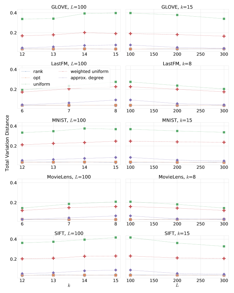
Figure 7.1. Total Variation Distance of the methods on the datasets. Parameter choices are $k=15,L=100$ for GLOVE, MNIST, SIFT and $k=8,L=100$ for Last.FM and MovieLens. Choices are varied to introduce more collisions.

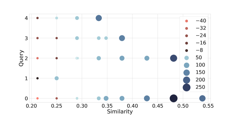
Figure 7.2. Scatter plot of differences in reported frequencies on Last.FM between uniform bucket (standard LSH) sampling and optimal (fair) sampling on five queries. $x$-axis: Similarity to query point; $y$-axis: id of the query. Each point represents the average difference in frequency among all points with the same similarity to a fixed query point. Darker and larger circles means large difference in report frequencies. Note large discrepancies for points at low and high similarity.

7.1. Output Distribution of Different Approaches (Q1)

We start by building the LSH data structure with the parameters detailed in the previous subsection. For each query $\mathbf{q}$, we first compute the number $M(\mathbf{q})$ of near neighbors that collide with the query point. Next, we repeat the query $\mathbf{q}$ $100M(\mathbf{q})$ times and collect the reported points.

Figure 7.1 provides an overview over the resulting output distribution of the five different approaches on the five datasets. Each data point is the total variation distance (or statistical distance) between the output distribution and the uniform distribution. Let us first concentrate on the standard choices $k=15,L=100$ for Euclidean distance and $k=8,L=100$ for Jaccard similarity. We make the following observations. Firstly, there is a clear difference in the output distribution between the (approximately) fair approaches and the two standard choices uniform and weighted uniform. On all datasets, there is a large deviation from the uniform distribution with large differences between the two approaches on the three Euclidean distance datasets, and a marginal differences on the two Jaccard similarity datasets. The degree approximation is much closer to the uniform distribution. The rank approach described in Section 3.1 is nearly indistinguishable from the independent sampling approach that uses exact degree computations. This means that on the used datasets there is little overlap between the neighborhood of the query points, and the dependence considerations discussed in Section 3.1 do not materialize.

As visible from the plot, we vary the parameters to introduce more collisions between the query and dataset points in the following two ways: We shorten the number of concatenated hash functions for a fixed number of repetitions, and we increase the number of repetitions for a fixed concatenation length. In both cases, the output distributions are closer to the uniform distribution.

Since it is difficult to argue about the unfairness of a distribution that is around .4 away in total variation distance from the uniform distribution, we provide a “zoomed in” visualization in Figure 7.2. In this plot, we show the difference in reported frequencies between the uniform/uniform approach and fair sampling for 5 out of the 50 queries on the Last.FM dataset. Note that using our querying approach, each point should be roughly reported 100 times. This is true for the fair sampling approach (with frequencies between 92 and 108), but we can clearly see a large difference to the standard sampling approach. This approach heavily under-reports points at lower similarity above the threshold .6 (only 60 reports on average), and heavily over-reports points at high similarity (360 reports in the maximum), which means that individually there is a difference of a factor of nearly 6 in the reported frequencies. This means that standard approaches will indeed yield biased neighborhoods in real-world situations. Using algorithms that solve the independent sampling version of the $r$-NN problem eliminate such bias.

7.2. Additional cost factor for solving the exact neighborhood variant (Q2)

The running time bounds of the algorithms in Section 5 and Section 6 have an additional additive or multiplicative running time factor $\tilde{O}(b_{S}(\mathbf{q},cr)/b_{S}(\mathbf{q},r))$, putting in relation the number of points at distance at most $cr,c\geq 1,$ (or similarity at least $cr,c\leq 1,$) to those at threshold $r$. The values $r$ and $cr$ are the distance/similarity thresholds picked when building the data structure. In general, a larger gap between $r$ and $cr$ makes the $n^{\rho}$ term in the running times smaller. However, the additive or multiplicative cost $\tilde{O}(b_{S}(\mathbf{q},cr)/b_{S}(\mathbf{q},r))$ can potentially be prohibitively large for worst-case datasets.

Figure 7.3 depicts the ratio of points with similarity at least $cr$ and $r$ for two of the real-world datasets (the other three showed similar behavior). We see that one has to be careful and choose a rather small approximation factor, since the ratio $b_{S}(\mathbf{q},cr)/b_{S}(\mathbf{q},r)$ can easily be the domination factor. For example, $c=2$ means that we may set $\mathsf{L}$ to roughly $n^{1/4}$, which is 10. The cost of the query is then dominated by the ratio of near and $cr$-near points. This shows that a careful inspection of dataset/query set characteristics might be necessary to find good parameter choices that balance cost terms.

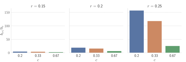
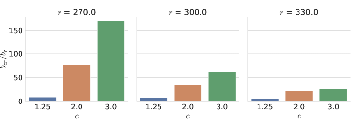
Figure 7.3. Top: Ratio of number of points with similarity at least $cr$ and number of points with similarity at least $r$ for $r\in\{0.15,0.2,0.25\}$ and $c=\{1/5,1/3,2/3\}$ for MovieLens. Bottom: Ratio of number of points distance at most $cr$ and number of points within distance $r$ for $r\in\{270,300,300\}$ and $c=\{1.25,2.0,3.0\}$ for SIFT. Note that similarity and distance behave inversely with regard to $r$ and $cr$.

7.3. Running time observations (Q3)

We implemented LSH for Euclidean distance in C ++ idea to compare running times in language that generates suitable fast code. We carry out the same number of queries as before, but repeat each experiment ten times. To simplify the code structure and the use of additional data structures, we made the following implementation choices: (i) In the rank data structure, we store each bucket as a list of points sorted by their rank. In the perturbation step, all buckets are sorted again after exchanging a rank. (ii) For the other data structures, we carry out a linear scan on the bucket sizes to select a bucket (by weight).

Figure 7.5 reports on the average query time needed by the different methods to answer the $100M(\mathbf{q})$ queries. These running times range from 10 to 100ms for the non-fair sampling methods, and they are about a magnitude larger for the (approximately) fair approaches. With respect to exact and approximate degree computation, we see that the former is around 1.5/2/3 times slower than the approximate approach on GLOVE, SIFT, and MNIST, respectively. The method using rank perturbation, which leads to similar distributions as the optimal exact degree computation in the considered workloads, is roughly as fast as the optimal variant on GLOVE, 2 times faster on SIFT, and 3 times faster on MNIST. On the SIFT dataset, it is roughly 2 times faster than approximating the degree and using rejection sampling.

With a smaller number of trials, we also compared our methods to a naïve approach that collects all colliding points, filters the near neighbors, and returns a uniform choice in the resulting set. This method resulted in running times that were roughly 2-3 times slower than the exact degree computation.

7.4. Fairness in the approximate version (Q4)

We turn our focus to the approximate neighborhood sampling problem. Recall that the algorithm may return points in $B(\mathbf{q},cr)\setminus B(\mathbf{q},r)$ as well, which speeds up the query since it avoids additional filtering steps. In the following, we will provide a concrete example that the output of an algorithm that solves this problem might yield unexpected sampling results.

Let us define the following dataset over the universe $\mathcal{U}=\{1,\ldots,30\}$: We let $\mathbf{X}=\{16,\ldots,30\}$, $\mathbf{Y}=\{1,\ldots,18\}$, and $\mathbf{Z}=\{1,\ldots,27\}$. Furthermore, we let $\mathcal{M}$ contain all subsets of $\mathbf{Y}$ having at least $15$ elements (excluding $\mathbf{Y}$ itself). The dataset is the collection of $\mathbf{X},\mathbf{Y},\mathbf{Z}$ and all sets in $\mathcal{M}$. Let the query $\mathbf{Q}$ be the set $\{1,\ldots,30\}$. To build the data structure, we set $r=0.9$ and $cr=0.5$. It is easy to see that $\mathbf{Z}$ is the nearest neighbor with similarity 0.9. $\mathbf{Y}$ is the second-nearest point with similarity 0.6, but $\mathbf{X}$ is among the points with the lowest similarity of 0.5. Finally, we note that each $\mathbf{x}\in\mathcal{M}$ has similarity ranging from 0.5 to $0.5\overline{6}$. Under the approximate neighborhood sampling problem, all points can be returned for the given query.

As in the previous subsection, the algorithm collects all the points found in the $\mathsf{L}$ buckets and returns a point picked uniformly at random among those points having similarity at least 0.5. Figure 7.5 shows the sampling probabilities of the sets $\mathbf{X},\mathbf{Y},\mathbf{Z}$. The plot clearly shows that the notion of approximate neighborhood does not provide a sensible guarantee on the individual fairness of users in this example. The set $\mathbf{X}$ is more than 50 times more likely than $\mathbf{Y}$ to be returned, even though $\mathbf{Y}$ is more similar to the query. This is due to the clustered neighborhood of $\mathbf{Y}$, making many other points appear at the same time in the buckets. On the other hand, $\mathbf{X}$ has no close points in its neighborhood (except $\mathbf{Z}$ and $\mathbf{Q}$).

We remark that we did not observe this influence of clustered neighborhoods on the real-world datasets. However, it is important to notice that approximate neighborhood could introduce unintentional bias and, furthermore, can be exploited by an adversary to discriminate a given user (e.g., an adversary can create a set of objects $\mathcal{M}$ that obfuscate a given entry $\mathbf{Y}$.)

Based on this example, one could argue that the observed sampling behavior is intentional. If the goal is to find good representatives in the neighborhood of the query, then it certainly seems preferable that $\mathbf{X}$ is reported with such high probability (which is roughly the same as all points in $\mathcal{M}$ and $\mathbf{Y}$ combined). Our notion of fairness would make the output less diverse, since $\mathbf{X}$ clearly stands out from many other points in the neighborhood, but it is supposed to be treated in the very same way. Such a trade-off between diversity and fairness was also observed, for example, by Leonhardt et al. (Leonhardt et al., 2018).

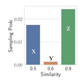
Figure 7.4. Empirical sampling probabilities of points $\mathbf{X},\mathbf{Y},\mathbf{Z}$.

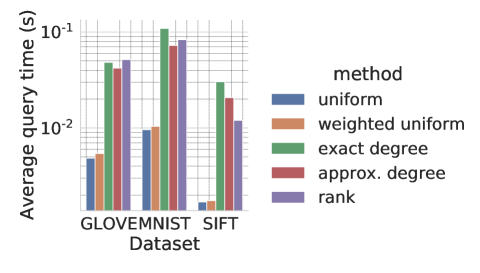
Figure 7.5. Comparison of average query times among the five methods on GLOVE, MNIST, and SIFT.

8. Conclusions

In this paper, we have investigated a possible definition of fairness in similarity search by connecting the notion of “equal opportunity” to independent range sampling. An interesting open question is to investigate the applicability of our data structures for problems like discrimination discovery (Luong et al., 2011), diversity in recommender systems (Adomavicius and Kwon, 2014), privacy preserving similarity search (Riazi et al., 2016), and estimation of kernel density (Charikar and Siminelakis, 2017). Moreover, it would be interesting to investigate techniques for providing incentives (i.e., reverse discrimination (Luong et al., 2011)) to prevent discrimination: an idea could be to merge the data structures in this paper with distance-sensitive hashing functions in (Aumüller et al., 2018), which allow to implement hashing schemes where the collision probability is an (almost) arbitrary function of the distance. Further, the techniques presented here require a manual trade-off between the performance of the LSH part and the additional running time contribution from finding the near points among the non-far points. From a user point of view, we would much rather prefer a parameterless version of our data structure that finds the best trade-off with small overhead, as discussed in (Ahle et al., 2017) in another setting. Finally, for some of the data structures presented here, the query time is also a function of the local density around the query point (e.g. $n\left({q,cr}\right)/n\left({q,r}\right)$), it would be ideal to find the optimal dependence on this local density.

Appendix A A linear space near-neighbor data structure

We will split up the analysis of the data structure from Section 6 into two parts. First, we describe and analyze a query algorithm that ignores the cost of storing and evaluating the $m$ random vectors. Next, we will describe and analyze the changes necessary to obtain an efficient query method as the one described in Section 6.

A.1. Description of the Data Structure

Construction

To set up the data structure for a point set $S\subseteq\mathbb{R}^{d}$ of $n$ data points and two parameters $\beta<\alpha$, choose $m\geq 1$ random vectors $\mathbf{a}_{1},\ldots,\mathbf{a}_{m}$ where each $\mathbf{a}=(a_{1},\ldots,a_{d})\sim\mathcal{N}(0,1)^{d}$ is a vector of $d$ independent and identically distributed standard normal Gaussians. For each $i\in\{1,\ldots,m\}$, let $L_{i}$ contain all data points $\mathbf{x}\in S$ such that $\langle{\mathbf{a}_{i}},{\mathbf{x}}\rangle$ is largest among all vectors $\mathbf{a}$.

Query

For a query point $\mathbf{q}\in\mathbb{R}^{d}$ and for a choice of $\varepsilon\in(0,1)$ controlling the success probability of the query, define $f(\alpha,\varepsilon)=\sqrt{2(1-\alpha^{2})\ln(1/\varepsilon)}$. Let $\Delta_{\mathbf{q}}$ be the largest inner product of $\mathbf{q}$ over all $\mathbf{a}$. Let $L^{\prime}_{1},\ldots,L^{\prime}_{K}$ denote the lists associated with random vectors $\mathbf{a}$ satisfying $\langle{\mathbf{a}},{\mathbf{q}}\rangle\geq\alpha\Delta_{q}-f(\alpha,\varepsilon)$. Check all points in $L^{\prime}_{1},\ldots,L^{\prime}_{K}$ and report the first point $\mathbf{x}$ such that $\langle{\mathbf{q}},{\mathbf{x}}\rangle\geq\beta$. If no such point exists, report $\perp$.

The proof of the theorem below will ignore the cost of evaluating $\mathbf{a}_{1},\ldots,\mathbf{a}_{m}$. An efficient algorithm for evaluating these vectors is provided in Appendix A.4.

Theorem 1.

Let $-1<\beta<\alpha<1$, $\varepsilon\in(0,1)$, and $n\geq 1$. Let $\rho=\frac{(1-\alpha^{2})(1-\beta^{2})}{(1-\alpha\beta)^{2}}$. There exists $m=m(n,\alpha,\beta)$ such that the data structure described above solves the $(\alpha,\beta)$-NN problem with probability at least $1-\varepsilon$ using space $O(m+n)$ and expected query time $n^{\rho+o(1)}$.

We split the proof up into multiple steps. First, we show that for every choice of $m$, inspecting the lists associated with those random vectors $\mathbf{a}$ such that their inner product with the query point $\mathbf{q}$ is at least the given query threshold guarantees to find a close point with probability at least $1-\varepsilon$. The next step is to show that the number of far points in these lists is $n^{\rho+o(1)}$ in expectation.

A.2. Analysis of Close Points

Lemma 0.

Given $m$ and $\alpha$, let $\mathbf{q}$ and $\mathbf{x}$ such that $\langle{\mathbf{q}},{\mathbf{x}}\rangle=\alpha$. Then we find $\mathbf{x}$ with probability at least $1-\varepsilon$ in the lists associated with vectors that have inner product at least $\alpha\Delta_{\mathbf{q}}-f(\alpha,\varepsilon)$ with $\mathbf{q}$.

Proof.

By spherical symmetry (Christiani, 2017), we may assume that $\mathbf{x}=(1,0,\ldots,0)$ and $\mathbf{q}=(\alpha,\sqrt{1-\alpha^{2}},0,$ $\ldots,0)$ . The probability of finding $\mathbf{x}$ when querying the data structure for $\mathbf{q}$ can be bounded as follows from below. Let $\Delta_{\mathbf{x}}$ be the largest inner product of $\mathbf{x}$ with vectors $\mathbf{a}$ and let $\Delta_{\mathbf{q}}$ be the largest inner product of $\mathbf{q}$ with these vectors. Given these thresholds, finding $\mathbf{x}$ is then equivalent to the statement that for the vector $\mathbf{a}$ with $\langle{\mathbf{a}},{\mathbf{x}}\rangle=\Delta_{\mathbf{x}}$ we have $\langle{\mathbf{a}},{\mathbf{q}}\rangle\geq\alpha\Delta_{\mathbf{q}}-f(\alpha,\varepsilon)$. We note that $\textnormal{Pr}\left[\max\{\langle{\mathbf{a}},{\mathbf{q}}\rangle\}=\Delta\right]=1-\textnormal{Pr}\left[\forall i:\langle{\mathbf{a}_{i}},{\mathbf{q}}\rangle<\Delta\right]$.

Thus, we may lower bound the probability of finding $\mathbf{x}$ for arbitrary choices $\Delta_{\mathbf{x}}$ and $\Delta_{\mathbf{q}}$ as follows:

$$\textnormal{Pr}\left[\text{find $\mathbf{x}$}\right] \geq\textnormal{Pr}\left[\langle{\mathbf{a}},{\mathbf{q}}\rangle\geq\alpha\Delta_{\mathbf{q}}{-}f(\alpha,\varepsilon)\mid\langle{\mathbf{a}},{\mathbf{x}}\rangle=\Delta_{\mathbf{x}}\text{ and }\langle{\mathbf{a}^{\prime}},{\mathbf{q}}\rangle=\Delta_{\mathbf{q}}\right]$$

(A.1) $$\quad-\textnormal{Pr}\left[\forall i:\langle{\mathbf{a}_{i}},{\mathbf{x}}\rangle<\Delta_{\mathbf{x}}\right]-\textnormal{Pr}\left[\forall i:\langle{\mathbf{a}_{i}},{\mathbf{q}}\rangle<\Delta_{\mathbf{q}}\right].$$

Here, we used that $\textnormal{Pr}\left[A\cap B\cap C\right]=1-\textnormal{Pr}\left[\overline{A}\cup\overline{B}\cup\overline{C}\right]\geq\textnormal{Pr}\left[A\right]-\textnormal{Pr}\left[\overline{B}\right]-\textnormal{Pr}\left[\overline{C}\right]$. We will now obtain bounds for the three terms on the right-hand side of Eq. (A.2) separately, but we first recall the following lemma from (Szarek and Werner, 1999):

Lemma 0 ((Szarek and Werner, 1999)).

Let $Z$ be a standard normal random variable. Then, for every $t\geq 0$, we have that

$$\frac{1}{\sqrt{2\pi}}\frac{1}{t+1}e^{-t^{2}/2}\leq\Pr(Z\geq t)\leq\frac{1}{\sqrt{\pi}}\frac{1}{t+1}e^{-t^{2}/2}.$$

Bounding the first term.

Since $\mathbf{q}=(\alpha,\sqrt{1-\alpha^{2}},0,\ldots,0)$ and $\mathbf{x}=(1,0,\ldots,0)$, the condition $\langle{\mathbf{a}},{\mathbf{x}}\rangle=\Delta_{\mathbf{x}}$ means that the first component of $\mathbf{a}$ is $\Delta_{\mathbf{x}}$. Thus, we have to bound the probability that a standard normal random variable $Z$ satisfies the inequality $\alpha\Delta_{\mathbf{x}}+\sqrt{1-\alpha^{2}}Z\geq\alpha\Delta_{\mathbf{q}}-f(\alpha,\varepsilon)$. Reordering terms, we get

$$Z\geq\frac{\alpha\Delta_{\mathbf{q}}-f(\alpha,\varepsilon)-\alpha\Delta_{\mathbf{x}}}{\sqrt{1-\alpha^{2}}}.$$

Choose $\Delta_{\mathbf{q}}=\Delta_{\mathbf{x}}$. In this case, we bound the probability that $Z$ is larger than a negative value. By symmetry of the standard normal distribution and using Lemma 3, we may compute

$$\textnormal{Pr}\left[Z\geq-\frac{f(\alpha,\varepsilon)}{\sqrt{1-\alpha^{2}}}\right] =1-\textnormal{Pr}\left[Z<-\frac{f(\alpha,\varepsilon)}{\sqrt{1-\alpha^{2}}}\right]$$

$$=1-\textnormal{Pr}\left[Z\geq\frac{f(\alpha,\varepsilon)}{\sqrt{1-\alpha^{2}}}\right]$$

(A.2) $$\geq 1-\frac{\text{Exp}\left(-\frac{(f(\alpha,\varepsilon))^{2}}{2(1-\alpha^{2})}\right)}{\sqrt{2\pi}\left(\frac{f(\alpha,\varepsilon)}{\sqrt{1-\alpha^{2}}}+1\right)}\geq 1-\varepsilon.$$

Bounding the second term and third term.

We first observe that

$$\textnormal{Pr}\left[\forall i:\langle{\mathbf{a}_{i}},{\mathbf{x}}\rangle<\Delta_{\mathbf{x}}\right] =\textnormal{Pr}\left[\langle{\mathbf{a}_{1}},{\mathbf{x}}\rangle<\Delta_{\mathbf{x}}\right]^{m}$$

$$=\left(1-\textnormal{Pr}\left[\langle{\mathbf{a}_{1}},{\mathbf{x}}\rangle\geq\Delta_{\mathbf{x}}\right]\right)^{m}$$

$$\leq\left(1-\frac{\text{Exp}[-\Delta_{\mathbf{x}}^{2}/2]}{\sqrt{2\pi}(\Delta_{x}+1)}\right)^{m}.$$

Setting $\Delta_{\mathbf{x}}=\sqrt{2\log m-\log(4\kappa\pi\log(m))}$ upper bounds this term by $\text{Exp}[-\sqrt{\kappa}]$. Thus, by setting $\kappa\geq\log^{2}(1/\delta)$ the second term is upper bounded by $\delta\in(0,1)$. The same thought can be applied to the third summand of Eq. (A.2), which is only smaller because of the negative offset $f(\alpha,\varepsilon)$.

Putting everything together.

Putting the bounds obtained for all three summands together shows that we can find $\mathbf{x}$ with probability at least $1-\varepsilon^{\prime}$ by choosing $\varepsilon$ and $\delta$ such that $\varepsilon^{\prime}\geq\varepsilon+2\delta$. ∎

A.3. Analysis of Far Points

Lemma 0.

Let $-1<\beta<\alpha<1$. There exists $m=m(n,\alpha,\beta)$ such that the expected number of points $\mathbf{x}$ with $\langle{\mathbf{x}},{\mathbf{q}}\rangle\leq\beta$ in $L^{\prime}_{1},\ldots,L^{\prime}_{K}$ where $K=|\{i\mid\langle{\mathbf{a}_{i}},{\mathbf{q}}\rangle\geq\alpha\Delta_{\mathbf{q}}-f(\alpha,\varepsilon)\}|$ is $n^{\rho+o(1)}$.

Proof.

We will first focus on a single far-away point $\mathbf{x}$ with inner product at most $\beta$. Again, let $\Delta_{\mathbf{q}}$ be the largest inner product of $\mathbf{q}$. Let $\mathbf{x}$ be stored in $L_{i}$. Then we find $\mathbf{x}$ if and only if $\langle{\mathbf{a}_{i}},{\mathbf{q}}\rangle\geq\alpha\Delta_{\mathbf{q}}-f(\alpha,\varepsilon).$ By spherical symmetry, we may assume that $\mathbf{x}=(1,0,\ldots,0)$ and $\mathbf{q}=(\beta,\sqrt{1-\beta^{2}},0,\ldots,0)$.

We first derive values $t_{\mathbf{q}}$ and $t_{\mathbf{x}}$ such that, with high probability, $\Delta_{\mathbf{q}}\geq t_{\mathbf{q}}$ and $\Delta_{\mathbf{x}}\leq t_{\mathbf{x}}$. From the proof of Lemma 2, we know that

$$\textnormal{Pr}\left[\max\{\langle{\mathbf{a}},{\mathbf{q}}\rangle\}\geq t\right] \leq 1-\left(1-\frac{\text{Exp}\left(-t^{2}/2\right)}{\sqrt{2\pi}(t+1)}\right)^{m}.$$

Setting $t_{\mathbf{q}}=\sqrt{2\log(m/\log(n))-\log(4\pi\log(m/\log n))}$ shows that with high probability we have $\Delta_{\mathbf{q}}\geq t_{\mathbf{q}}$. Similarly, the choice $t_{\mathbf{x}}=\sqrt{2\log(m\log(n))-\log(4\pi\log(m\log n))}$ is with high probability at least $\Delta_{\mathbf{x}}$. In the following, we condition on the event that $\Delta_{\mathbf{q}}\geq t_{\mathbf{q}}$ and $\Delta_{\mathbf{x}}\leq t_{\mathbf{x}}$.

We may bound the probability of finding $\mathbf{x}$ as follows:

$$\textnormal{Pr}\left[\langle{\mathbf{a}},{\mathbf{q}}\rangle\geq\alpha\Delta_{\mathbf{q}}-f(\alpha,\varepsilon)\mid\langle{\mathbf{a}},{\mathbf{x}}\rangle=\Delta_{\mathbf{x}}\right]\leq$$

$$\leq\textnormal{Pr}\left[\langle{\mathbf{a}},{\mathbf{q}}\rangle\geq\alpha\Delta_{\mathbf{q}}-f(\alpha,\varepsilon)\mid\langle{\mathbf{a}},{\mathbf{x}}\rangle=t_{\mathbf{x}}\right]$$

$$\leq\textnormal{Pr}\left[\langle{\mathbf{a}},{\mathbf{q}}\rangle\geq\alpha t_{\mathbf{q}}-f(\alpha,\varepsilon)\mid\langle{\mathbf{a}},{\mathbf{x}}\rangle=t_{\mathbf{x}}\right].$$

Given that $\langle{\mathbf{a}},{\mathbf{x}}\rangle$ is $t_{\mathbf{x}}$, the condition $\langle{\mathbf{a}},{\mathbf{q}}\rangle\geq\alpha t_{\mathbf{q}}-f(\alpha,\varepsilon)$ is equivalent to the statement that for a standard normal variable $Z$ we have $Z\geq\frac{(\alpha t_{\mathbf{q}}-f(\alpha,\varepsilon)-\beta t_{\mathbf{x}})}{\sqrt{1-\beta^{2}}}$. Using Lemma 3, we have

$$\textnormal{Pr}\left[\langle{\mathbf{a}},{\mathbf{q}}\rangle\geq\alpha t_{\mathbf{q}}-f(\alpha,\varepsilon)\mid\langle{\mathbf{a}},{\mathbf{x}}\rangle=t_{\mathbf{x}}\right]\leq\frac{\text{Exp}\left(-\frac{(\alpha t_{\mathbf{q}}-f(\alpha,\varepsilon)-\beta t_{\mathbf{x}})^{2}}{2(1-\beta^{2})}\right)}{\sqrt{\pi}\left(\frac{(\alpha t_{\mathbf{q}}-f(\alpha,\varepsilon)-\beta t_{\mathbf{x}})}{\sqrt{1-\beta^{2}}}+1\right)}$$

$$\hskip 20.00003pt\leq\text{Exp}\left(-\frac{(\alpha t_{\mathbf{q}}-f(\alpha,\varepsilon)-\beta t_{\mathbf{x}})^{2}}{2(1-\beta^{2})}\right)$$

$$\hskip 20.00003pt\stackrel{{\scriptstyle(1)}}{{=}}\text{Exp}\left(-\frac{(\alpha-\beta)^{2}t_{\mathbf{x}}^{2}}{2(1-\beta^{2})}\left(1+O(1/\log\log n)\right)\right)$$

(A.3) $$\hskip 20.00003pt=\left(\frac{1}{m}\right)^{\frac{(\alpha-\beta)^{2}}{1-\beta^{2}}+o(1)},$$

where step (1) follows from the observation that $t_{\mathbf{q}}/t_{\mathbf{x}}=1+O(1/\log\log n)$ and $f(\alpha,\varepsilon)/t_{\mathbf{x}}=O(1/\log\log n)$ if $m=\Omega(\log n)$.

Next, we want to balance this probability with the expected cost for checking all lists where the inner product with the associated vector $\mathbf{a}$ is at least $\alpha\Delta_{\mathbf{q}}-f(\alpha,\varepsilon)$. By linearity of expectation, the expected number of lists to be checked is not more than

$$m\cdot\text{Exp}\left(-(\alpha t_{\mathbf{q}})^{2}\left(1/2-f(\alpha,\varepsilon)/(\alpha t_{\mathbf{q}})+f(\alpha,\varepsilon)^{2}/(2(\alpha t_{\mathbf{q}})^{2})\right)\right),$$

which is $m^{1-\alpha^{2}+o(1)}$ using the value of $t_{\mathbf{q}}$ set above. This motivates to set Eq. (A.3) equal to $m^{1-\alpha^{2}}/n$, taking into account that there are at most $n$ far-away points. Solving for $m$, we get $m=n^{\frac{1-\beta^{2}}{(1-\alpha\beta)^{2}}+o(1)}$ and this yields $m^{1-\alpha^{2}+o(1)}=n^{\rho+o(1)}$. ∎

A.4. Efficient Evaluation

The previous subsections assumed that $m$ filters can be evaluated and stored for free. However, this requires space and time $n^{(1-\beta^{2})/(1-\alpha\beta)^{2}}$, which is much higher than the work we expect from checking the points in all filters above the threshold. We solve this problem by using the tensoring approach, which can be seen as a simplified version of the general approach proposed in (Christiani, 2017).

Construction

Let $t=\lceil 1/(1-\alpha^{2})\rceil$ and assume that $m^{1/t}$ is an integer. Consider $t$ independent data structures $\mathcal{D}_{1},\ldots,\mathcal{D}_{t}$, each using $m^{1/t}$ random vectors $\mathbf{a}_{i,j}$, for $i\in\{1,\ldots,t\},j\in[m^{1/t}]$. Each $\mathcal{D}_{i}$ is instantiated as described above. During preprocessing, consider each $\mathbf{x}\in S$. If $\mathbf{a}_{1,i_{1}},\ldots,\mathbf{a}_{t,i_{t}}$ are the random vectors that achieve the largest inner product with $\mathbf{x}$ in $\mathcal{D}_{1},\ldots,\mathcal{D}_{t}$, map the index of $\mathbf{x}$ in $S$ to the bucket $(i_{1},\ldots,i_{t})\in[m^{1/t}]^{t}$. Use a hash table to keep track of all non-empty buckets. Since each data point in $S$ is stored exactly once, the space usage is $O(n+tm^{1/t})$.

Query

Given the query point $\mathbf{q}$, evaluate all $tm^{1/t}$ filters. For $i\in\{1,\ldots,t\}$, let $\mathcal{I}_{i}=\{j\mid\langle{\mathbf{a}_{i,j}},{\mathbf{q}}\rangle\geq\alpha\Delta_{\mathbf{q},i}-f(\alpha,\varepsilon)\}$ be the set of all indices of filters that are above the individual query threshold in $\mathcal{D}_{i}$. Check all buckets $(i_{1},\ldots,i_{t})\in\mathcal{I}_{1}\times\dots\times\mathcal{I}_{t}$. If there is a bucket containing a close point, return it, otherwise return $\perp$.

Theorem 5.

Let $S\subseteq X$ with $|S|=n$ and $-1<\beta<\alpha<1$. The tensoring data structure solves the $(\alpha,\beta)$-NN problem in linear space and expected time $n^{\rho+o(1)}$.

Before proving the theorem, we remark that efficient evaluation comes at the price of lowering the success probability from a constant $p$ to $p^{1/(1-\alpha^{2})}$. Thus, for $\delta\in(0,1)$ repeating the construction $\ln(1/\delta)p^{1-\alpha^{2}}$ times yields a success probability of at least $1-\delta$.

Proof.

Observe that with the choice of $m$ as in the proof of Lemma 4, we can bound $m^{1/t}=n^{(1-\alpha^{2})(1-\beta^{2})/(1-\alpha\beta)^{2}+o(1)}=n^{\rho+o(1)}$. This means that preprocessing takes time $n^{1+\rho+o(1)}$. Moreover, the additional space needed for storing the $tm^{1/t}$ random vectors is $n^{\rho+o(1)}$ as well. For a given query point $\mathbf{q}$, we expect that each $\mathcal{I}_{i}$ is of size $m^{(1-\alpha^{2})/t+o(1)}$. Thus, we expect to check not more than $m^{1-\alpha^{2}+o(1)}=n^{\rho+o(1)}$ buckets in the hash table, which shows the stated claim about the expected running time.

Let $\mathbf{x}$ be a point with $\langle{\mathbf{q}},{\mathbf{x}}\rangle\geq\alpha$. The probability of finding $\mathbf{x}$ is the probability that the vector associated with $\mathbf{x}$ has inner product at least $\alpha\Delta_{\mathbf{q},i}-f(\alpha,\varepsilon)$ in $\mathcal{D}_{i}$, for all $i\in\{1,\ldots,t\}$. This probability is $p^{t}$, where $p$ is the probability of finding $\mathbf{x}$ in a single data structure $\mathcal{D}_{i}$. By Theorem 1 and since $\alpha$ is a constant, this probability is constant and can be bounded from below by $1-\delta$ via a proper choice of $\varepsilon$ as discussed in the proof of Lemma 2.

Let $\mathbf{y}$ be a point with $\langle{\mathbf{q}},{\mathbf{y}}\rangle<\beta$. Using the same approach in the proof of Lemma 4, we observe that the probability of finding $\mathbf{y}$ in an individual $\mathcal{D}_{i}$ is $(1/m)^{1/t\cdot(\alpha-\beta)^{2}/(1-\beta^{2})+o(1)}$. Thus the probability of finding $\mathbf{y}$ in a bucket inspected for $\mathbf{q}$ is at most $(1/m)^{(\alpha-\beta)^{2}/(1-\beta^{2})+o(1)}$. Setting parameters as before shows that we expect at most $n^{\rho+o(1)}$ far points in buckets inspected for query $\mathbf{q}$, which completes the proof. ∎

References

- (1)
- Abiteboul et al. (2017) Serge Abiteboul, Marcelo Arenas, Pablo Barceló, Meghyn Bienvenu, Diego Calvanese, Claire David, Richard Hull, Eyke Hüllermeier, Benny Kimelfeld, Leonid Libkin, Wim Martens, Tova Milo, Filip Murlak, Frank Neven, Magdalena Ortiz, Thomas Schwentick, Julia Stoyanovich, Jianwen Su, Dan Suciu, Victor Vianu, and Ke Yi. 2017. Research Directions for Principles of Data Management (Abridged). SIGMOD Rec. 45, 4 (2017), 5–17.
- Adar (2007) Eytan Adar. 2007. User 4xxxxx9: Anonymizing query logs. (01 2007). http://www2007.org/workshops/paper_52.pdf Appeared in the workshop Query Log Analysis: Social and Technological Challenges, in association with WWW 2007.
- Adomavicius and Kwon (2014) Gediminas Adomavicius and YoungOk Kwon. 2014. Optimization-based approaches for maximizing aggregate recommendation diversity. INFORMS Journal on Computing 26, 2 (2014), 351–369.
- Afshani and Phillips (2019) Peyman Afshani and Jeff M. Phillips. 2019. Independent Range Sampling, Revisited Again. In 35th International Symposium on Computational Geometry, SoCG 2019, June 18-21, 2019, Portland, Oregon, USA (LIPIcs, Vol. 129), Gill Barequet and Yusu Wang (Eds.). Schloss Dagstuhl - Leibniz-Zentrum für Informatik, Wadern, Germany, 4:1–4:13. https://doi.org/10.4230/LIPIcs.SoCG.2019.4
- Afshani and Wei (2017) Peyman Afshani and Zhewei Wei. 2017. Independent Range Sampling, Revisited. In 25th Annual European Symposium on Algorithms, ESA 2017, September 4-6, 2017, Vienna, Austria (LIPIcs, Vol. 87), Kirk Pruhs and Christian Sohler (Eds.). Schloss Dagstuhl - Leibniz-Zentrum fuer Informatik, Wadern, Germany, 3:1–3:14. https://doi.org/10.4230/LIPIcs.ESA.2017.3
- Agarwal et al. (2018) Alekh Agarwal, Alina Beygelzimer, Miroslav Dudík, John Langford, and Hanna M. Wallach. 2018. A Reductions Approach to Fair Classification. In Proc. 35th Int. Conf. Mach. Learning (ICML) (Proc. of Mach. Learn. Research, Vol. 80), Jennifer G. Dy and Andreas Krause (Eds.). PMLR, , 60–69. http://proceedings.mlr.press/v80/agarwal18a.html
- Ahle et al. (2017) Thomas D. Ahle, Martin Aumüller, and Rasmus Pagh. 2017. Parameter-Free Locality Sensitive Hashing for Spherical Range Reporting. In Proceedings of the Twenty-Eighth Annual ACM-SIAM Symposium on Discrete Algorithms (Barcelona, Spain) (SODA ’17). Society for Industrial and Applied Mathematics, USA, 239–256.
- Alman and Williams (2015) Josh Alman and Ryan Williams. 2015. Probabilistic Polynomials and Hamming Nearest Neighbors. In Proceedings of the 2015 IEEE 56th Annual Symposium on Foundations of Computer Science (FOCS) (FOCS ’15). IEEE Computer Society, USA, 136–150. https://doi.org/10.1109/FOCS.2015.18
- Andoni (2005) Alexandr Andoni. 2005. E2LSH 0.1 User manual. (2005). https://www.mit.edu/~andoni/LSH/manual.pdf
- Andoni and Indyk (2008) A. Andoni and P. Indyk. 2008. Near-optimal hashing algorithms for approximate nearest neighbor in high dimensions. Commun. ACM 51, 1 (2008), 117–122. https://doi.org/10.1145/1327452.1327494
- Andoni et al. (2017) Alexandr Andoni, Thijs Laarhoven, Ilya Razenshteyn, and Erik Waingarten. 2017. Optimal Hashing-Based Time-Space Trade-Offs for Approximate near Neighbors. In Proceedings of the Twenty-Eighth Annual ACM-SIAM Symposium on Discrete Algorithms (Barcelona, Spain) (SODA ’17). Society for Industrial and Applied Mathematics, USA, 47–66.
- Aumüller et al. (2020a) Martin Aumüller, Erik Bernhardsson, and Alexander John Faithfull. 2020a. ANN-Benchmarks: A benchmarking tool for approximate nearest neighbor algorithms. Inf. Syst. 87 (2020), 17. https://doi.org/10.1016/j.is.2019.02.006
- Aumüller et al. (2018) Martin Aumüller, Tobias Christiani, Rasmus Pagh, and Francesco Silvestri. 2018. Distance-Sensitive Hashing. In Proc. 37th ACM Symposium on Principles of Database Systems (PODS). Association for Computing Machinery, New York, NY, USA, 89–104.
- Aumüller et al. (2020b) Martin Aumüller, Rasmus Pagh, and Francesco Silvestri. 2020b. Fair Near Neighbor Search: Independent Range Sampling in High Dimensions. In Proceedings of the 39th ACM SIGMOD-SIGACT-SIGAI Symposium on Principles of Database Systems, PODS 2020, Portland, OR, USA, June 14-19, 2020, Dan Suciu, Yufei Tao, and Zhewei Wei (Eds.). ACM, New York, NY, USA, 191–204. https://doi.org/10.1145/3375395.3387648
- Backurs et al. (2019) Arturs Backurs, Piotr Indyk, Krzysztof Onak, Baruch Schieber, Ali Vakilian, and Tal Wagner. 2019. Scalable Fair Clustering. In Proceedings of the 36th International Conference on Machine Learning, ICML 2019, 9-15 June 2019, Long Beach, California, USA (Proceedings of Machine Learning Research, Vol. 97), Kamalika Chaudhuri and Ruslan Salakhutdinov (Eds.). PMLR, , 405–413. http://proceedings.mlr.press/v97/backurs19a.html
- Bar-Yossef et al. (2002) Ziv Bar-Yossef, T. S. Jayram, Ravi Kumar, D. Sivakumar, and Luca Trevisan. 2002. Counting Distinct Elements in a Data Stream. In Proceedings of the 6th International Workshop on Randomization and Approximation Techniques (RANDOM ’02). Springer-Verlag, Berlin, Heidelberg, 1–10.
- Beame et al. (2017) Paul Beame, Sariel Har-Peled, Sivaramakrishnan Natarajan Ramamoorthy, Cyrus Rashtchian, and Makrand Sinha. 2017. Edge Estimation with Independent Set Oracles. CoRR abs/1711.07567 (2017), 29. arXiv:1711.07567 http://arxiv.org/abs/1711.07567
- Bera et al. (2019) Suman Kalyan Bera, Deeparnab Chakrabarty, Nicolas Flores, and Maryam Negahbani. 2019. Fair Algorithms for Clustering. In Advances in Neural Information Processing Systems 32: Annual Conference on Neural Information Processing Systems 2019, NeurIPS 2019, December 8-14, 2019, Vancouver, BC, Canada, Hanna M. Wallach, Hugo Larochelle, Alina Beygelzimer, Florence d’Alché-Buc, Emily B. Fox, and Roman Garnett (Eds.). Curran Associates, Inc., Red Hook, NY, USA, 4955–4966. http://papers.nips.cc/paper/8741-fair-algorithms-for-clustering
- Broder (1997) Andrei Z. Broder. 1997. On the resemblance and containment of documents. In Proc. Compression and Complexity of Sequences. IEEE Computer Society, USA, 21–29.
- Charikar (2002) Moses Charikar. 2002. Similarity estimation techniques from rounding algorithms. In Proc. 34th ACM Symposium on Theory of Computing (STOC). ACM, USA, 380–388.
- Charikar and Siminelakis (2017) Moses Charikar and Paris Siminelakis. 2017. Hashing-Based-Estimators for Kernel Density in High Dimensions. In 58th IEEE Annual Symposium on Foundations of Computer Science, FOCS 2017, Berkeley, CA, USA, October 15-17, 2017, Chris Umans (Ed.). IEEE Computer Society, USA, 1032–1043. https://doi.org/10.1109/FOCS.2017.99
- Chierichetti et al. (2017) Flavio Chierichetti, Ravi Kumar, Silvio Lattanzi, and Sergei Vassilvitskii. 2017. Fair Clustering through Fairlets. In Proceedings of the 31st International Conference on Neural Information Processing Systems (Long Beach, California, USA) (NIPS’17). Curran Associates Inc., Red Hook, NY, USA, 5036–5044.
- Chierichetti et al. (2019) Flavio Chierichetti, Ravi Kumar, Silvio Lattanzi, and Sergei Vassilvtiskii. 2019. Matroids, Matchings, and Fairness. In Proceedings of Machine Learning Research (Proceedings of Machine Learning Research, Vol. 89), Kamalika Chaudhuri and Masashi Sugiyama (Eds.). PMLR, , 2212–2220. http://proceedings.mlr.press/v89/chierichetti19a.html
- Chouldechova (2017) Alexandra Chouldechova. 2017. Fair prediction with disparate impact: A study of bias in recidivism prediction instruments. Big data 5, 2 (2017), 153–163.
- Christiani (2017) Tobias Christiani. 2017. A Framework for Similarity Search with Space-Time Tradeoffs using Locality-Sensitive Filtering. In Proc. 28th Symposium on Discrete Algorithms (SODA). Society for Industrial and Applied Mathematics, USA, 31–46.
- Datar et al. (2004) M. Datar, N. Immorlica, P. Indyk, and V. S. Mirrokni. 2004. Locality-sensitive hashing scheme based on -stable distributions. In Proc. 20th Annu. Sympos. Comput. Geom. (SoCG) (Brooklyn, New York, USA). ACM, New York, NY, USA, 253–262. https://doi.org/10.1145/997817.997857
- David and Nagaraja (2004) Herbert Aron David and Haikady Navada Nagaraja. 2004. Order statistics (3rd ed.). John Wiley & Sons, New York, NY.
- Donini et al. (2018) Michele Donini, Luca Oneto, Shai Ben-David, John Shawe-Taylor, and Massimiliano Pontil. 2018. Empirical Risk Minimization under Fairness Constraints. In Proceedings of the 32nd International Conference on Neural Information Processing Systems (Montréal, Canada) (NIPS’18). Curran Associates Inc., Red Hook, NY, USA, 2796–2806.
- Dwork et al. (2012) Cynthia Dwork, Moritz Hardt, Toniann Pitassi, Omer Reingold, and Richard Zemel. 2012. Fairness through Awareness. In Proceedings of the 3rd Innovations in Theoretical Computer Science Conference (Cambridge, Massachusetts) (ITCS ’12). Association for Computing Machinery, New York, NY, USA, 214–226. https://doi.org/10.1145/2090236.2090255
- Elzayn et al. (2019) Hadi Elzayn, Shahin Jabbari, Christopher Jung, Michael Kearns, Seth Neel, Aaron Roth, and Zachary Schutzman. 2019. Fair Algorithms for Learning in Allocation Problems. In Proceedings of the Conference on Fairness, Accountability, and Transparency. ACM, Association for Computing Machinery, New York, NY, USA, 170–179. https://doi.org/10.1145/3287560.3287571
- Eshghi and Rajaram (2008) Kave Eshghi and Shyamsundar Rajaram. 2008. Locality Sensitive Hash Functions Based on Concomitant Rank Order Statistics. In Proceedings of the 14th ACM SIGKDD International Conference on Knowledge Discovery and Data Mining (Las Vegas, Nevada, USA) (KDD ’08). Association for Computing Machinery, New York, NY, USA, 221–229. https://doi.org/10.1145/1401890.1401921
- Everitt et al. (2009) Brian S. Everitt, Sabine Landau, and Morven Leese. 2009. Cluster Analysis (4th ed.). Wiley Publishing, Chicago, IL.
- Flajolet and Martin (1985) Philippe Flajolet and G. Nigel Martin. 1985. Probabilistic Counting Algorithms for Data Base Applications. J. Comput. Syst. Sci. 31, 2 (1985), 182–209.
- Friedler et al. (2016) Sorelle A. Friedler, Carlos Scheidegger, and Suresh Venkatasubramanian. 2016. On the (im)possibility of fairness. CoRR abs/1609.07236 (2016), 16. arXiv:1609.07236 http://arxiv.org/abs/1609.07236
- Har-Peled et al. (2012) S. Har-Peled, P. Indyk, and R. Motwani. 2012. Approximate Nearest Neighbors: Towards Removing the Curse of Dimensionality. Theory Comput. 8, Article 14 (2012), 30 pages. https://doi.org/10.4086/toc.2012.v008a014 Special issue in honor of Rajeev Motwani.
- Har-Peled and Mahabadi (2019) Sariel Har-Peled and Sepideh Mahabadi. 2019. Near Neighbor: Who is the Fairest of Them All?. In Proc. 32th Neural Info. Proc. Sys. (NeurIPS), Hanna M. Wallach, Hugo Larochelle, Alina Beygelzimer, Florence d’Alché-Buc, Emily B. Fox, and Roman Garnett (Eds.). Curran Associates, Inc., Red Hook, NY, USA, 13176–13187. http://papers.nips.cc/paper/9476-near-neighbor-who-is-the-fairest-of-them-all
- Hardt et al. (2016) Moritz Hardt, Eric Price, and Nati Srebro. 2016. Equality of Opportunity in Supervised Learning. In Neural Info. Proc. Sys. (NIPS), Daniel D. Lee, Masashi Sugiyama, Ulrike von Luxburg, Isabelle Guyon, and Roman Garnett (Eds.). Curran Associates Inc., Red Hook, NY, USA, 3315–3323. http://papers.nips.cc/paper/6374-equality-of-opportunity-in-supervised-learning
- Harel and Koren (2001) David Harel and Yehuda Koren. 2001. On Clustering Using Random Walks. In FSTTCS 2001: Foundations of Software Technology and Theoretical Computer Science, 21st Conference, Bangalore, India, December 13-15, 2001, Proceedings (Lecture Notes in Computer Science, Vol. 2245), Ramesh Hariharan, Madhavan Mukund, and V. Vinay (Eds.). Springer, NY, 18–41. https://doi.org/10.1007/3-540-45294-X_3
- Hassanat et al. (2014) Ahmad Basheer Hassanat, Mohammad Ali Abbadi, Ghada Awad Altarawneh, and Ahmad Ali Alhasanat. 2014. Solving the Problem of the K Parameter in the KNN Classifier Using an Ensemble Learning Approach. CoRR abs/1409.0919 (2014), 33–39. arXiv:1409.0919 http://arxiv.org/abs/1409.0919
- Hu et al. (2014) Xiaocheng Hu, Miao Qiao, and Yufei Tao. 2014. Independent range sampling. In Proceedings of the 33rd ACM SIGMOD-SIGACT-SIGART Symposium on Principles of Database Systems, PODS’14, Snowbird, UT, USA, June 22-27, 2014, Richard Hull and Martin Grohe (Eds.). ACM, New York, NY, USA, 246–255. https://doi.org/10.1145/2594538.2594545
- Huang et al. (2006) Jiayuan Huang, Alexander J. Smola, Arthur Gretton, Karsten M. Borgwardt, and Bernhard Scholkopf. 2006. Correcting Sample Selection Bias by Unlabeled Data. In Proceedings of the 19th International Conference on Neural Information Processing Systems (Canada) (NIPS’06). MIT Press, Cambridge, MA, USA, 601–608.
- Indyk and Motwani (1998) Piotr Indyk and Rajeev Motwani. 1998. Approximate Nearest Neighbors: Towards Removing the Curse of Dimensionality. In Proceedings of the Thirtieth Annual ACM Symposium on Theory of Computing (Dallas, Texas, USA) (STOC ’98). Association for Computing Machinery, New York, NY, USA, 604–613. https://doi.org/10.1145/276698.276876
- Kannan et al. (2019) Sampath Kannan, Aaron Roth, and Juba Ziani. 2019. Downstream Effects of Affirmative Action. In Proceedings of the Conference on Fairness, Accountability, and Transparency (Atlanta, GA, USA) (FAT* ’19). Association for Computing Machinery, New York, NY, USA, 240–248. https://doi.org/10.1145/3287560.3287578
- Keeling and Eames (2005) Matt J Keeling and Ken T.D Eames. 2005. Networks and epidemic models. Journal of The Royal Society Interface 2, 4 (Sept. 2005), 295–307. https://doi.org/10.1098/rsif.2005.0051
- Kleinberg et al. (2017) Jon Kleinberg, Himabindu Lakkaraju, Jure Leskovec, Jens Ludwig, and Sendhil Mullainathan. 2017. Human decisions and machine predictions. The quarterly journal of economics 133, 1 (2017), 237–293.
- Kleindessner et al. (2019) Matthäus Kleindessner, Samira Samadi, Pranjal Awasthi, and Jamie Morgenstern. 2019. Guarantees for Spectral Clustering with Fairness Constraints. In Proceedings of the 36th International Conference on Machine Learning (Proceedings of Machine Learning Research, Vol. 97), Kamalika Chaudhuri and Ruslan Salakhutdinov (Eds.). PMLR, Long Beach, California, USA, 3458–3467. http://proceedings.mlr.press/v97/kleindessner19b.html
- Knuth (1998) Donald Ervin Knuth. 1998. The art of computer programming, Volume II: Seminumerical Algorithms, 3rd Edition. Addison-Wesley, Boston, MA. https://www.worldcat.org/oclc/312898417
- Koren et al. (2009) Yehuda Koren, Robert M. Bell, and Chris Volinsky. 2009. Matrix Factorization Techniques for Recommender Systems. IEEE Computer 42, 8 (2009), 30–37.
- Kung et al. (2012) Yi-Hung Kung, Pei-Sheng Lin, and Cheng-Hsiung Kao. 2012. An optimal -nearest neighbor for density estimation. Statistics & Probability Letters 82, 10 (2012), 1786 – 1791. https://doi.org/10.1016/j.spl.2012.05.017
- LeCun et al. (1998) Yann LeCun, Léon Bottou, Yoshua Bengio, and Patrick Haffner. 1998. Gradient-based learning applied to document recognition. Proc. IEEE 86, 11 (1998), 2278–2324.
- Leonhardt et al. (2018) Jurek Leonhardt, Avishek Anand, and Megha Khosla. 2018. User Fairness in Recommender Systems. In Companion Proceedings of the The Web Conference 2018 (Lyon, France) (WWW ’18). International World Wide Web Conferences Steering Committee, Republic and Canton of Geneva, CHE, 101–102. https://doi.org/10.1145/3184558.3186949
- Li and König (2010) Ping Li and Christian König. 2010. B-Bit Minwise Hashing. In Proceedings of the 19th International Conference on World Wide Web (Raleigh, North Carolina, USA) (WWW ’10). Association for Computing Machinery, New York, NY, USA, 671–680. https://doi.org/10.1145/1772690.1772759
- Luong et al. (2011) Binh Thanh Luong, Salvatore Ruggieri, and Franco Turini. 2011. K-NN as an Implementation of Situation Testing for Discrimination Discovery and Prevention. In Proceedings of the 17th ACM SIGKDD International Conference on Knowledge Discovery and Data Mining (San Diego, California, USA) (KDD ’11). Association for Computing Machinery, New York, NY, USA, 502–510. https://doi.org/10.1145/2020408.2020488
- Munoz et al. (2016) Cecilia Munoz, Megan Smith, and DJ Patil. 2016. Big Data: A Report on Algorithmic Systems, Opportunity, and Civil Rights. Executive Office of the President and Penny Hill Press, Damascus, MD.
- of the President (2016) Executive Office of the President. 2016. Big data: A report on algorithmic systems, opportunity, and civil rights.
- Olfat and Aswani (2019) Matt Olfat and Anil Aswani. 2019. Convex Formulations for Fair Principal Component Analysis. Proceedings of the AAAI Conference on Artificial Intelligence 33, 01 (Jul. 2019), 663–670. https://doi.org/10.1609/aaai.v33i01.3301663
- Olken and Rotem (1995a) Frank Olken and Doron Rotem. 1995a. Random sampling from databases: a survey. Statistics and Computing 5, 1 (1995), 25–42.
- Olken and Rotem (1995b) Frank Olken and Doron Rotem. 1995b. Sampling from spatial databases. Statistics and Computing 5, 1 (01 Mar 1995), 43–57. https://doi.org/10.1007/BF00140665
- Pennington et al. (2014) Jeffrey Pennington, Richard Socher, and Christopher Manning. 2014. GloVe: Global Vectors for Word Representation. In Proceedings of the 2014 Conference on Empirical Methods in Natu ral Language Processing (EMNLP). Association for Computational Linguistics, Doha, Qatar, 1532–1543. https://doi.org/10.3115/v1/D14-1162
- Pleiss et al. (2017) Geoff Pleiss, Manish Raghavan, Felix Wu, Jon Kleinberg, and Kilian Q. Weinberger. 2017. On Fairness and Calibration. In Proceedings of the 31st International Conference on Neural Information Processing Systems (Long Beach, California, USA) (NIPS’17). Curran Associates Inc., Red Hook, NY, USA, 5684–5693.
- Qi and Atallah (2008) Yinian Qi and Mikhail J. Atallah. 2008. Efficient Privacy-Preserving k-Nearest Neighbor Search. In Proceedings of the 2008 The 28th International Conference on Distributed Computing Systems (ICDCS ’08). IEEE Computer Society, USA, 311–319. https://doi.org/10.1109/ICDCS.2008.79
- Riazi et al. (2016) M. Sadegh Riazi, Beidi Chen, Anshumali Shrivastava, Dan S. Wallach, and Farinaz Koushanfar. 2016. Sub-Linear Privacy-Preserving Near-Neighbor Search with Untrusted Server on Large-Scale Datasets. (2016). ArXiv:1612.01835.
- Selbst et al. (2019) Andrew D. Selbst, Danah Boyd, Sorelle A. Friedler, Suresh Venkatasubramanian, and Janet Vertesi. 2019. Fairness and Abstraction in Sociotechnical Systems. In Proceedings of the Conference on Fairness, Accountability, and Transparency (Atlanta, GA, USA) (FAT* ’19). Association for Computing Machinery, New York, NY, USA, 59–68. https://doi.org/10.1145/3287560.3287598
- Shakhnarovich et al. (2006) Gregory Shakhnarovich, Trevor Darrell, and Piotr Indyk. 2006. Nearest-neighbor methods in learning and vision: theory and practice (neural information processing). The MIT Press, Cambridge, MA.
- Szarek and Werner (1999) Stanislaw J. Szarek and Elisabeth Werner. 1999. A Nonsymmetric Correlation Inequality for Gaussian Measure. Journal of Multivariate Analysis 68, 2 (1999), 193 – 211.
- Torralba and Efros (2011) A. Torralba and A. A. Efros. 2011. Unbiased Look at Dataset Bias. In Proceedings of the 2011 IEEE Conference on Computer Vision and Pattern Recognition (CVPR ’11). IEEE Computer Society, USA, 1521–1528. https://doi.org/10.1109/CVPR.2011.5995347
- Williams (2005) Ryan Williams. 2005. A New Algorithm for Optimal 2-constraint Satisfaction and Its Implications. Theor. Comput. Sci. 348, 2 (2005), 357–365.
- Zafar et al. (2017) Muhammad Bilal Zafar, Isabel Valera, Manuel Gomez-Rodriguez, and Krishna P. Gummadi. 2017. Fairness Beyond Disparate Treatment & Disparate Impact: Learning Classification without Disparate Mistreatment. In Proceedings of the 26th International Conference on World Wide Web, WWW 2017, Perth, Australia, April 3-7, 2017, Rick Barrett, Rick Cummings, Eugene Agichtein, and Evgeniy Gabrilovich (Eds.). International World Wide Web Conferences Steering Committee, Republic and Canton of Geneva, CHE, 1171–1180. https://doi.org/10.1145/3038912.3052660