Exploring the AGN-Merger Connection in Arp 245 I: Nuclear Star Formation and Gas Outflow in NGC 2992

Abstract

Galaxy mergers are central to our understanding of galaxy formation, especially within the context of hierarchical models. Besides having a large impact on the star formation history, mergers are also able to influence gas motions at the centre of galaxies and trigger an Active Galactic Nucleus (AGN). In this paper, we present a case study of the Seyfert galaxy NGC 2992, which together with NGC 2993 forms the early-stage merger system Arp 245. Using Gemini Multi-Object Spectrograph (GMOS) integral field unit (IFU) data from the inner 1.1 kpc of the galaxy we were able to spatially resolve the stellar populations, the ionisation mechanism and kinematics of ionised gas. From full spectral synthesis, we found that the stellar population is primarily composed by old metal-rich stars (t $\geq$ 1.4 Gyr, $Z\geq 2.0$ ${\rm Z_{\odot}}$), with a contribution of at most 30 per cent of the light from a young and metal-poor population (t $\leq$ 100 Myr, $Z\leq 1.0$ ${\rm Z_{\odot}}$). We detect H$\alpha$ and H$\beta$ emission from the Broad Line Region (BLR) with a Full Width at Half Maximum (FWHM) of $\sim$ 2000 $\rm km\,s^{-1}$. The Narrow Line Region (NLR) kinematics presents two main components: one from gas orbiting the galaxy disk and a blueshifted (velocity $\approx$ -200 $\rm km\,s^{-1}$) outflow, possibly correlated with the radio emission, with mass outflow rate of $\sim$ 2 M_⊙ yr^-1 and a kinematic power of $\sim$ 2 $\times 10^{40}$ erg s^-1 ($\dot{E}_{out}$/$L_{bol}$ $\approx$ 0.2 per cent). We also show even though the main ionisation mechanism is the AGN radiation, ionisation by young stars and shocks may also contribute to the emission line ratios presented in the innermost region of the galaxy.

1 Introduction

The vast majority of galaxies with a spheroid host a supermassive black hole (SMBH) in their centres, with a mass range of $\sim 10^{6}-10^{10}\,\,{\rm M_{\odot}}$. In some galaxies, these objects are active and emit intense radiation due to the accretion of matter onto the SMBH through an inner region called accretion disk (Begelman et al., 1984; Peterson et al., 1998; Event Horizon Telescope Collaboration et al., 2019). Active galactic nuclei (AGN) in Seyfert galaxies are classified as type 1 and 2, depending on the presence of broad emission lines of the Balmer series, with intermediate types between these two also possible; these broad lines are produced in a region called Broad Line Region (BLR).

The importance of AGN in the evolution of the host galaxy is not completely understood, but there is evidence pointing to a co-evolution scenario between the two. The $M_{\rm BH}-\sigma_{*}$ relation (Ferrarese & Merritt, 2000; Kormendy & Ho, 2013) – which relates the mass of the SMBH with the stellar velocity dispersion in the galactic bulge – and the simultaneous peak between star formation rate (SFR) and SMBH accretion rate in cosmological studies at $z\approx 2$ (Silverman et al., 2008; Madau & Dickinson, 2014) are some of the indications towards a causal connection between host galaxy evolution and of its SMBH.

The energy released by the AGN in the form of radiation, winds, or radio plasma jets is known to impact on the interstellar medium of the host galaxy. All these processes are collectively known as feedback. The role of such AGN feedback in the evolution of galaxies, however, is still a subject of ongoing debate. AGN feedback may be a key factor in quenching star formation, mainly in the late stages of the host galaxy’s evolution (Di Matteo et al., 2005; Croton et al., 2006). In fact, large scale hydrodynamic simulations of galaxy formation are not able to reproduce observed properties of massive galaxies if AGN feedback models are not included (Springel et al., 2005; Bullock & Boylan-Kolchin, 2017) in which these processes are responsible for suppressing the growth of the most massive galaxies by heating and expelling the gas that would form more stars. Powerful AGN driven winds are a possible mechanism for preventing further growth of the host galaxy. These winds can have outflow velocities as high as 1000 $\rm km\,s^{-1}$(Rupke & Veilleux, 2011; Greene et al., 2012) and as low as well $\approx 100-200$ $\rm km\,s^{-1}$, with mass outflow rates in nearby galaxies averaging at a few solar masses per year (e.g. Riffel & Storchi-Bergmann, 2011; Crenshaw et al., 2015; Revalski et al., 2018).

Theoretical studies suggest large scale events like major mergers are the dominant processes leading to SMBH growth at high masses (Menci et al., 2014). At high redshifts (z > 2), major mergers have also been proposed as fuelling mechanisms of the fastest-growing SMBHs (Treister et al., 2012). A major merger can destabilise large quantities of gas, driving massive inflows towards the nuclear region of galaxies and triggering bursts of star formation and nuclear activity (Hopkins & Quataert, 2010; Blumenthal & Barnes, 2018). Many studies have found that the most luminous AGN are preferentially hosted by galaxy mergers (Schawinski et al., 2010; Glikman et al., 2015; Fan et al., 2016). At lower luminosities, several studies have found a higher incidence of galaxies with signatures of interactions in AGN hosts as compared to control samples (Koss et al., 2010) and particularly in close galaxy pairs (Ellison et al., 2011; Satyapal et al., 2014) suggesting kinematic pairs are conducive environments for black hole growth.

One possible consequence of gas inflow is the circumnuclear star formation (Hopkins et al., 2008; Hopkins & Quataert, 2010). Such merger-driven inflows can both increase the star formation rate (Ellison et al., 2013; Pan et al., 2019) and modify the metallicities gradients of the galaxies (Barrera-Ballesteros et al., 2015). However, classical emission-line SFR probes (e.g. Kennicutt, 1998) and metallicity calibrations (e.g. Alloin et al., 1979; Pettini & Pagel, 2004) cannot be applied to active galaxies, due to the contamination of the AGN ionisation to the emission lines. In this way, the use of stellar populations synthesis, by performing full spectral fitting, can reveal clues on the star formation history (SFH) and chemical evolution of AGN host galaxies and its content.

In this context, we present high spatial and spectral resolution optical IFU observations of the inner 1.1 kpc of NGC 2992. NGC 2992 is a nearby interacting Seyfert galaxy seen almost edge-on ($i\sim 70^{\circ}$, Marquez et al., 1998) at a distance, as measured using the Tully-Fisher relation, of $38\,\,{\rm Mpc}$ (Theureau et al., 2007), which translates into a projected angular scale of $\sim$ 150 pc per arcsec. Alongside with the starburst galaxy NGC 2993 and the tidal dwarf galaxy A245N it forms the system Arp 245. Using hydrodynamic simulations, Duc et al. (2000) reported the system is currently at an early stage of the interaction, about $\approx 100\,\,{\rm Myr}$ after pericentre passage. Nevertheless, tidal tails have already developed, which can be seen by optical images (Fig. 1), in CO and HI lines (Duc et al., 2000) and infrared (IR) images (García-Bernete et al., 2015).

The galaxy nuclear activity has been the subject of several studies, partly due to its variability as seen both in X-rays and in the optical (Trippe et al., 2008), even leading to changes in spectral classification. Early spectra published by Shuder (1980), Veron et al. (1980), and Ward et al. (1980) all show the presence of a weak broad H$\alpha$ component, originated in the BLR, but no detectable corresponding broad H$\beta$ component, leading to its original classification as a Seyfert 1.9. Observations from 1994 (Allen et al., 1999), however, display no broad H$\alpha$ component, thus having the classification of Seyfert 2. Gilli et al. (2000) reported a broad H$\alpha$ emission again, just to disappear once again when observed in 2006 by L. Trippe et al. (2008). More recently Schnorr-Müller et al. (2016), after subtracting the narrow component, were able to detect the broad H$\beta$ component for the first time, then classifying the galaxy as a Seyfert 1.8.

In the radio, 6 cm observations show a double lobe 8-shaped structure of about 8 arcsec ($\sim$ 1 kpc) extension to the northwest and Southeast of the galaxy, along position angle (PA) of $-26^{\circ}$ (Ulvestad & Wilson, 1984). From IR observations, Chapman et al. (2000) suggest the best interpretation is that this structure is related to expanding plasma bubbles, possibly carried by internal jets from the AGN. More recently, using radio polarimetry, Irwin et al. (2017) found another double-lobed radio morphology within its spiral disc, which was revealed in linearly polarized emission but not in total intensity emission. This second structure by Irwin et al. (2017) is much more extended than the one found by Ulvestad & Wilson (1984) reaching several kpcs from the nucleus, being interpreted by the authors as a relic of an earlier episode of AGN activity.

NGC 2992 gas kinematics is complex as found by several long slit spectroscopy studies (e.g. Marquez et al., 1998; Veilleux et al., 2001) as well as by several Integral Field Unit observations (García-Lorenzo et al., 2001; Friedrich et al., 2010; Müller-Sánchez et al., 2011). These observations show, at most positions, the presence of a double component line profile. While one component follows the galaxy rotation curve, the other is interpreted as outflowing gas by the authors. Using The Multi Unit Spectroscopic Explorer (MUSE Bacon et al., 2010) at the Very Larga Telescope (VLT) Mingozzi et al. (2019) clearly show the presence of a kpc-scale, bipolar outflow with a large opening angle.

This paper is the first in a series which will explore the possible connection between merger and AGN in Arp 245. In this first paper, we analyse both the stellar populations and the properties of the ionised gas of NGC 2992, in order to better understand the physical conditions of the nuclear region and the mutual role of nuclear activity and the interaction may play. In a second paper (Guolo-Pereira et al., in prep., Paper II) we will observationally explore the effects of the interaction in NGC 2993. While in the third one (Lösch et al., in prep, Paper III) we will present a modern version of the hydrodynamics simulations by Duc et al. (2000) focusing on the possible triggering of the AGN during the merger.

The present paper is organised as follows: in section 2 we describe the observations and data reduction; section 3 we present the stellar populations synthesis and its spatial distribution; the ionised gas kinematics is described in section 4; ionisation mechanisms are discussed in section 5; section 6 presents our discussion of the main results and their significance; and finally section 7 contains our conclusions.

2 Observations and data reduction

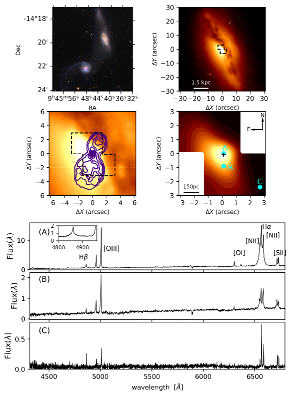
Figure 1: Top Left: LRGB image composition of Arp 245 from Block (2011). Top Right: GMOS r’ band acquisition image of NGC 2992. Middle Left: Zoomed acquisition image, and the Ulvestad & Wilson (1984) radio emission in purple (contours : 3, 6, 9, 15, 30, 50, 70, 90 per cent of the peak of 7.2 mJy). The dashed rectangles show the two IFU FoV’s. Middle Right: IFU continuum mean flux in the FoV. The black cross represents the continuum nuclear position in all figures of the paper. All maps of the paper were smoothed using a Gaussian kernel with FHWM with half of the spatial resolution, see section 2. Bottom, from top to bottom: Spectra corresponding to the regions marked as A, B and C, with spectral flux density in units of $10^{-15}$ $\rm erg\,s^{-1}\,cm^{-2}\,\textup{\AA}^{-1}$. North is up and East to the left in this and all figures of the paper.

This work is mostly based on data obtained with the Integral Field Unit (IFU) of the Gemini Multi Object Spectrograph (GMOS) at the Gemini South telescope on the night of February 15, 2018 (Gemini project GS-2018A-Q-208, P.I. Ruschel-Dutra). The observations consisted of two adjacent IFU fields (covering 5″$\times$ 3$\aas@@fstack{\prime\prime}$5 each). The fields are slightly offset, both in Right Ascension (RA) and Declination (Dec), in order to increase the field of view (FoV) and cover a larger portion of the galaxy plane. For each IFU field, there are six exposures, with an integration time of 560 seconds each. Each science observation is accompanied by a 5 $\times$ 1$\aas@@fstack{\prime\prime}$75 sky observation for atmospheric lines removal.

The spatial resolution is limited by seeing, which was at $0\aas@@fstack{\prime\prime}8$ during the observations, corresponding to 120 pc at the galaxy. The observed spectra covered a range from 4075 to 7285 Å with an instrumental dispersion $\sigma_{\rm instr}\approx 40\,\,\rm km\,s^{-1}$, obtained from the Copper-Argon arc lamp lines.

The reduction procedures were performed using the Gmos Ifu REDuction Suite (GIREDS). The process comprised the usual steps: bias subtraction, flatfielding, trimming, wavelength calibration, telluric emission subtraction, relative flux calibration, the building of the data cubes, and finally the registering and combination of the 12 individual exposures. The final cube was built with a spatial sampling of $0\aas@@fstack{\prime\prime}1\times 0\aas@@fstack{\prime\prime}1$, resulting in a FoV with $\approx 2800$ spaxels. After cropping the borders and superimposing the FoVs, it results in a total useful combined FoV, with total angular coverage of 29 arcsec² around the nucleus. The combined FoV is centred at RA = 9h45m42s and Dec = -14^o9′3″, while the continuum peak is shifted at $\Delta$RA = 0.1″and $\Delta$Dec = -0.1″.

Many Gemini data cubes show certain “instrumental fingerprints”, in the form of vertical stripes in the reconstructed data cube. Such features also have specific spectral signatures. In order to identify and remove these instrumental features, we use a technique based on Principal Component Analysis (PCA, Menezes et al., 2014). The fingerprint removal is fundamental for the stellar population synthesis because its effect is more apparent for lower instrumental counts. The data cube spectra were corrected for Galactic extinction using the Cardelli et al. (1989) extinction curve (CCM) for an $A_{V}=0.166$ (Schlafly & Finkbeiner, 2011) and by Doppler effect using the radial velocity of 2345 $\rm km\,s^{-1}$(see section 4).

We show in the upper panel of the Fig. 1 an LRGB image of the Arp 245 system (Left) and the acquisition image taken with a r’ filter (Right). In the middle panel we show a zoomed version of the acquisition image superimposed with the the Ulvestad & Wilson (1984) figure of 8-shaped radio emission of the galaxy (Left) and the mean continuum flux in the IFU’s FoV (Right), while in the bottom panels we show three sample spectra from representative regions marked, respectively from top to bottom, A, B and C. The prominent dust lane seen in the acquisition image, and in the stellar continuum image from the IFU, has a reported $A_{V}$ greater than 3 (Colina et al., 1987; Schnorr-Müller et al., 2016). Spectra from this region of high extinction have no measurable stellar component above the noise level, as exemplified by the spectrum extracted from C. The nuclear spectrum shows a broad H${\alpha}$ component, and a faint broad H$\beta$ is also present, in contrast with its original Seyfert 1.9 classification but in agreement with its the current state, Seyfert 1.8, proposed by Schnorr-Müller et al. (2016).

3 Stellar Populations

In order to obtain the spatially resolved SFH, and to fit the gas emission features, free from the stellar population contamination, we performed stellar population synthesis on the data cube by employing the starlight full spectra fitting code (Cid Fernandes et al., 2005).

Briefly, starlight fits an observed stellar spectrum $O_{\lambda}$ with a model $M_{\lambda}$ built from a linear combination of $N$ spectral components. Dust attenuation is treated as if due to a foreground screen and parametrised by the $V$-band extinction $A_{V}$. Stellar kinematics is modelled with a Gaussian line-of-sight velocity distribution centred at velocity $v_{*}$, and with a dispersion $\sigma_{*}$. Besides the model spectrum $M_{\lambda}$, the code outputs the corresponding values of $A_{V}$, $v_{\star}$, $\sigma_{\star}$, and a population vector $\vec{x}$ containing the percentage contribution of each base population to the flux at a chosen normalisation wavelength $\lambda_{0}$, which in our fits was chosen as $\lambda_{0}$ = 5500 Å. The code minimises the $\chi^{2}$ of the fit, though a more convenient and intuitive figure of merit to assess the quality of the fit is through adev parameter, defined as the mean value of $\left|O_{\lambda}-M_{\lambda}\right|/O_{\lambda}$ over the fitted wavelengths.

We note that, while there are many different spectral fitting codes and techniques available, cross-comparison of these various techniques have shown to yield rather consistent results (e.g. Koleva et al., 2008; Ferré-Mateu et al., 2012; Maksym et al., 2014; Mentz et al., 2016; Cid Fernandes, 2018). Therefore, rather than trying different fitting codes, we chose to maintain starlight and investigate the differences introduced by the choice of models and stellar libraries, which are known to produce variations in the recovered properties (e.g. Maraston & Strömbäck, 2011; Chen et al., 2010; Wilkinson et al., 2017; Baldwin et al., 2018; Dametto et al., 2019).

3.1 Evolutionary Models, Stellar Libraries and Featureless Continuum

This section discusses the stellar population models and stellar libraries used in this work, and how we can account for the contribution of a featureless continuum due to the AGN in NGC 2992.

The key ingredients in the stellar population synthesis method are the spectral base elements, i.e. those spectra available to the fitting code to combine in order to recover the galaxy properties. The base elements are, usually, Simple Stellar Population (SSP), i.e. a collection of stars with same age and metallicity, taken from an evolutionary model which are constructed using a stellar spectra library and an Initial Mass Function (IMF).

In this work we have used SSPs from two models: Bruzual & Charlot (2003, BC03), which uses the STELIB (Le Borgne et al., 2003) spectral library, and Maraston & Strömbäck (2011, M11), which employs the MILES (Sánchez-Blázquez et al., 2006) spectral library. For both models/libraries we use the same Chabrier (2003) IMF and instantaneous star formation bursts. We found varying the IMF produces only minor variations in the recovered SFH when compared to the changes introduced by using distinct models. The former is outside the scope of this work, and we refer the reader interested in this particular effect to Chen et al. (2010), Ge et al. (2019) and references therein. From the SSPs provided by BC03 we choose a set of 45 representative elements divided into three metallicities ($0.2,1.0,2.5$ ${\rm Z_{\odot}}$) and an age range covering from t(Gyr) $=0.001$ to t(Gyr) $=13$. From those available by M11 with the MILES library we chose a set of 40 SSPs with age and metallicity coverage as similar as possible to the BC03 ones: three metallicities ($0.5,1.0,2.0$ ${\rm Z_{\odot}}$) and ages ranging from t(Gyr) $=0.007$ to t(Gyr) $=13$. The complete list of SSPs used from each model is shown in LABEL:table:SSPs. It is important to mention that the MILES Library does not provide metal-poor stars ($Z=0.5$ ${\rm Z_{\odot}}$) younger than 55 Myr (0.055 Gyr), and neither metal-rich stars ($Z=2.0$ ${\rm Z_{\odot}}$) younger than 100 Myr (0.1 Gyr), while BC03/STELIB provide the same age range for the three metallicities (see LABEL:table:SSPs).

We define a reduced population vector with three age ranges: $t<$ 100  Myr;  100 Myr  $\leq t\leq$ 1.4 Gyr; and $\ t>1.4$ Gyr, to obtain a more robust description of the SFH than that obtained with the full population vector (see, e.g. Cid Fernandes et al., 2005), as well as to facilitate the visualisation of the spatially resolved fit results. The population vector components are denoted by $x_{Y}$, $x_{I}$ and $x_{O}$, where $`Y^{\prime}$, $`I^{\prime}$ and $`O^{\prime}$ stands for young, intermediate and old respectively. The division in a reduced population vector has been used in several works in stellar population synthesis (e.g. Cid Fernandes et al., 2005; Riffel et al., 2010a; Cid Fernandes et al., 2013; González Delgado et al., 2015; Mallmann et al., 2018), while the range values may be slightly distinct from one another, the ones adopted here are the most common. Also, for the young population the cutting value of 100 Myr is the estimated age of the pericentre passage between NGC2992 and its companion (Duc et al., 2000).

Table 1: SSPs used in the stellar population synthesis.

Model	BC03			M11
Spectral Library	STELIB			MILES
Metallicity ($Z_{\odot}$)	0.2	1.0	2.5	0.5	1.0	2.0
Ages (Gyr)	[rgb]0.2,0.2,0.20.001, 0.003, 0.005, [rgb]0.2,0.2,0.2[rgb]0.2,0.2,0.2[rgb]0.2,0.2,0.20.01, 0.025,  0.04, [rgb]0.2,0.2,0.2[rgb]0.2,0.2,0.2[rgb]0.2,0.2,0.2[rgb]0.2,0.2,0.2[rgb]0.2,0.2,0.2[rgb]0.2,0.2,0.20.1, 0.3, 0.6, 0.9, [rgb]0.2,0.2,0.2[rgb]0.2,0.2,0.2[rgb]0.2,0.2,0.2[rgb]0.2,0.2,0.2[rgb]0.2,0.2,0.2[rgb]0.2,0.2,0.2[rgb]0.2,0.2,0.2[rgb]0.2,0.2,0.2[rgb]0.2,0.2,0.2[rgb]0.2,0.2,0.21.5, 3.0, 5.0, [rgb]0.2,0.2,0.2[rgb]0.2,0.2,0.2[rgb]0.2,0.2,0.2[rgb]0.2,0.2,0.2[rgb]0.2,0.2,0.2[rgb]0.2,0.2,0.2[rgb]0.2,0.2,0.2[rgb]0.2,0.2,0.2[rgb]0.2,0.2,0.2[rgb]0.2,0.2,0.2[rgb]0.2,0.2,0.2[rgb]0.2,0.2,0.2[rgb]0.2,0.2,0.2[rgb]0.2,0.2,0.2[rgb]0.2,0.2,0.211.0, 13.0			[rgb]0.2,0.2,0.20.055, 0.065, [rgb]0.2,0.2,0.2[rgb]0.2,0.2,0.2[rgb]0.2,0.2,0.20.075, 0.085, [rgb]0.2,0.2,0.2[rgb]0.2,0.2,0.2[rgb]0.2,0.2,0.2[rgb]0.2,0.2,0.2[rgb]0.2,0.2,0.2[rgb]0.2,0.2,0.2 0.1, 0.15, [rgb]0.2,0.2,0.2[rgb]0.2,0.2,0.2[rgb]0.2,0.2,0.2[rgb]0.2,0.2,0.2[rgb]0.2,0.2,0.2[rgb]0.2,0.2,0.2[rgb]0.2,0.2,0.2[rgb]0.2,0.2,0.2[rgb]0.2,0.2,0.2[rgb]0.2,0.2,0.2 0.3, 0.6, [rgb]0.2,0.2,0.2[rgb]0.2,0.2,0.2[rgb]0.2,0.2,0.2[rgb]0.2,0.2,0.2[rgb]0.2,0.2,0.2[rgb]0.2,0.2,0.2[rgb]0.2,0.2,0.2[rgb]0.2,0.2,0.2[rgb]0.2,0.2,0.2[rgb]0.2,0.2,0.2[rgb]0.2,0.2,0.2[rgb]0.2,0.2,0.2[rgb]0.2,0.2,0.2[rgb]0.2,0.2,0.2[rgb]0.2,0.2,0.20.9	[rgb]0.2,0.2,0.20.007, 0008, [rgb]0.2,0.2,0.2[rgb]0.2,0.2,0.2[rgb]0.2,0.2,0.20.009, 0.01, [rgb]0.2,0.2,0.2[rgb]0.2,0.2,0.2[rgb]0.2,0.2,0.2[rgb]0.2,0.2,0.2[rgb]0.2,0.2,0.2[rgb]0.2,0.2,0.20.015, 0.025, [rgb]0.2,0.2,0.2[rgb]0.2,0.2,0.2[rgb]0.2,0.2,0.2[rgb]0.2,0.2,0.2[rgb]0.2,0.2,0.2[rgb]0.2,0.2,0.2[rgb]0.2,0.2,0.2[rgb]0.2,0.2,0.2[rgb]0.2,0.2,0.2[rgb]0.2,0.2,0.20.04, 0.055, [rgb]0.2,0.2,0.2[rgb]0.2,0.2,0.2[rgb]0.2,0.2,0.2[rgb]0.2,0.2,0.2[rgb]0.2,0.2,0.2[rgb]0.2,0.2,0.2[rgb]0.2,0.2,0.2[rgb]0.2,0.2,0.2[rgb]0.2,0.2,0.2[rgb]0.2,0.2,0.2[rgb]0.2,0.2,0.2[rgb]0.2,0.2,0.2[rgb]0.2,0.2,0.2[rgb]0.2,0.2,0.2[rgb]0.2,0.2,0.20.065, 0.075, [rgb]0.2,0.2,0.2[rgb]0.2,0.2,0.2[rgb]0.2,0.2,0.2[rgb]0.2,0.2,0.2[rgb]0.2,0.2,0.2[rgb]0.2,0.2,0.2[rgb]0.2,0.2,0.2[rgb]0.2,0.2,0.2[rgb]0.2,0.2,0.2[rgb]0.2,0.2,0.2[rgb]0.2,0.2,0.2[rgb]0.2,0.2,0.2[rgb]0.2,0.2,0.2[rgb]0.2,0.2,0.2[rgb]0.2,0.2,0.2[rgb]0.2,0.2,0.2[rgb]0.2,0.2,0.2[rgb]0.2,0.2,0.2[rgb]0.2,0.2,0.2[rgb]0.2,0.2,0.2[rgb]0.2,0.2,0.20.085, 0.1, [rgb]0.2,0.2,0.2[rgb]0.2,0.2,0.2[rgb]0.2,0.2,0.2[rgb]0.2,0.2,0.2[rgb]0.2,0.2,0.2[rgb]0.2,0.2,0.2[rgb]0.2,0.2,0.2[rgb]0.2,0.2,0.2[rgb]0.2,0.2,0.2[rgb]0.2,0.2,0.2[rgb]0.2,0.2,0.2[rgb]0.2,0.2,0.2[rgb]0.2,0.2,0.2[rgb]0.2,0.2,0.2[rgb]0.2,0.2,0.2[rgb]0.2,0.2,0.2[rgb]0.2,0.2,0.2[rgb]0.2,0.2,0.2[rgb]0.2,0.2,0.2[rgb]0.2,0.2,0.2[rgb]0.2,0.2,0.2[rgb]0.2,0.2,0.2[rgb]0.2,0.2,0.2[rgb]0.2,0.2,0.2[rgb]0.2,0.2,0.2[rgb]0.2,0.2,0.2[rgb]0.2,0.2,0.2[rgb]0.2,0.2,0.20.15, 0.3, 0.9, [rgb]0.2,0.2,0.2[rgb]0.2,0.2,0.2[rgb]0.2,0.2,0.2[rgb]0.2,0.2,0.2[rgb]0.2,0.2,0.2[rgb]0.2,0.2,0.2[rgb]0.2,0.2,0.2[rgb]0.2,0.2,0.2[rgb]0.2,0.2,0.2[rgb]0.2,0.2,0.2[rgb]0.2,0.2,0.2[rgb]0.2,0.2,0.2[rgb]0.2,0.2,0.2[rgb]0.2,0.2,0.2[rgb]0.2,0.2,0.2[rgb]0.2,0.2,0.2[rgb]0.2,0.2,0.2[rgb]0.2,0.2,0.2[rgb]0.2,0.2,0.2[rgb]0.2,0.2,0.2[rgb]0.2,0.2,0.2[rgb]0.2,0.2,0.2[rgb]0.2,0.2,0.2[rgb]0.2,0.2,0.2[rgb]0.2,0.2,0.2[rgb]0.2,0.2,0.2[rgb]0.2,0.2,0.2[rgb]0.2,0.2,0.2[rgb]0.2,0.2,0.2[rgb]0.2,0.2,0.2[rgb]0.2,0.2,0.2[rgb]0.2,0.2,0.2[rgb]0.2,0.2,0.2[rgb]0.2,0.2,0.2[rgb]0.2,0.2,0.2[rgb]0.2,0.2,0.21.5, 3.0, 5.0, [rgb]0.2,0.2,0.2[rgb]0.2,0.2,0.2[rgb]0.2,0.2,0.2[rgb]0.2,0.2,0.2[rgb]0.2,0.2,0.2[rgb]0.2,0.2,0.2[rgb]0.2,0.2,0.2[rgb]0.2,0.2,0.2[rgb]0.2,0.2,0.2[rgb]0.2,0.2,0.2[rgb]0.2,0.2,0.2[rgb]0.2,0.2,0.2[rgb]0.2,0.2,0.2[rgb]0.2,0.2,0.2[rgb]0.2,0.2,0.2[rgb]0.2,0.2,0.2[rgb]0.2,0.2,0.2[rgb]0.2,0.2,0.2[rgb]0.2,0.2,0.2[rgb]0.2,0.2,0.2[rgb]0.2,0.2,0.2[rgb]0.2,0.2,0.2[rgb]0.2,0.2,0.2[rgb]0.2,0.2,0.2[rgb]0.2,0.2,0.2[rgb]0.2,0.2,0.2[rgb]0.2,0.2,0.2[rgb]0.2,0.2,0.2[rgb]0.2,0.2,0.2[rgb]0.2,0.2,0.2[rgb]0.2,0.2,0.2[rgb]0.2,0.2,0.2[rgb]0.2,0.2,0.2[rgb]0.2,0.2,0.2[rgb]0.2,0.2,0.2[rgb]0.2,0.2,0.2[rgb]0.2,0.2,0.2[rgb]0.2,0.2,0.2[rgb]0.2,0.2,0.2[rgb]0.2,0.2,0.2[rgb]0.2,0.2,0.2[rgb]0.2,0.2,0.2[rgb]0.2,0.2,0.2[rgb]0.2,0.2,0.2[rgb]0.2,0.2,0.211.0, 13.0	[rgb]0.2,0.2,0.20.1, 0.15, [rgb]0.2,0.2,0.2[rgb]0.2,0.2,0.2[rgb]0.2,0.2,0.2 0.3, 0.6, [rgb]0.2,0.2,0.2[rgb]0.2,0.2,0.2[rgb]0.2,0.2,0.2[rgb]0.2,0.2,0.2[rgb]0.2,0.2,0.2[rgb]0.2,0.2,0.20.9, 1.5, [rgb]0.2,0.2,0.2[rgb]0.2,0.2,0.2[rgb]0.2,0.2,0.2[rgb]0.2,0.2,0.2[rgb]0.2,0.2,0.2[rgb]0.2,0.2,0.2[rgb]0.2,0.2,0.2[rgb]0.2,0.2,0.2[rgb]0.2,0.2,0.2[rgb]0.2,0.2,0.23.0, 5.0, [rgb]0.2,0.2,0.2[rgb]0.2,0.2,0.2[rgb]0.2,0.2,0.2[rgb]0.2,0.2,0.2[rgb]0.2,0.2,0.2[rgb]0.2,0.2,0.2[rgb]0.2,0.2,0.2[rgb]0.2,0.2,0.2[rgb]0.2,0.2,0.2[rgb]0.2,0.2,0.2[rgb]0.2,0.2,0.2[rgb]0.2,0.2,0.2[rgb]0.2,0.2,0.2[rgb]0.2,0.2,0.2[rgb]0.2,0.2,0.211.0, 13.0

When dealing with stellar populations in Seyfert galaxies, a power law ($F_{\lambda}\propto\lambda^{-\alpha}$) featureless continuum (FC) should be added to the spectral base (Koski, 1978) to account for the AGN emission. Values for $\alpha$ are between $0.5-2.0$ (Osterbrock & Ferland, 2006), with many authors working with large samples of galaxies assuming a general value of $\alpha=1.5$ (Storchi-Bergmann et al., 2003; Raimann et al., 2003; Cid Fernandes et al., 2004; Mallmann et al., 2018). Since this work is focused on a single object, we propose a method to specifically fit the $\alpha$ index for the optical spectrum of NGC 2992. We extracted two integrated spectra: an inner one, hereafter $S(\lambda)$, defined as the sum of spectra within a circular region with radius of 0$\aas@@fstack{\prime\prime}$4, and an external one, $E(\lambda)$, in an annulus with inner radius of 1″and outer radius of 1$\aas@@fstack{\prime\prime}$4, both centred at the peak of continuum emission. We model the $S(\lambda)$ spectrum as a combination of $E(\lambda)$ and a power law FC ($F_{\lambda}\propto\lambda^{-\alpha}$), both reddened by the same factor and normalised in the same wavelength, $\lambda_{0}=5500$ Å, as follows:

$$\left(\frac{S_{m}(\lambda)}{S_{m}(\lambda_{0})}\right)\\ =\left[\left(1-\boldsymbol{p}\right)\left(\frac{E(\lambda)}{E(\lambda_{0})}\right)+\boldsymbol{p}\left(\frac{\lambda}{\lambda_{0}}\right)^{-\boldsymbol{\alpha}}\right]\times 10^{-0.4\boldsymbol{\delta A_{V}}q_{\lambda}}$$ (1)

where $S_{m}(\lambda)$ is the model spectrum, $p$ is the fraction contribution of the FC, $\delta A_{V}$ is the difference in extinction between the $S(\lambda)$ and $E(\lambda)$ regions. The values which minimise the residuals between $S(\lambda)$ and $S_{m}(\lambda)$ are $p$ = 0.23, $\delta A_{V}$ = 2.2 and $\alpha$ =1.7.

It should be noted we are over-simplifying by assuming that $S(\lambda)$ is the combination of $E(\lambda)$ and an FC, i.e. the stellar spectrum of both are the same. However, we argue this is just a method to get a data-based value for $\alpha$, instead of just assuming a fixed value which is even less physically justified. Also, no further interpretation will be given in this regard besides the adoption of this $\alpha$ value to produce the FC base element.

3.2 Spatially Resolved Stellar Populations Synthesis

In order to perform the spatially resolved stellar synthesis with enough signal to noise ratio ($S/N$) we employed the Voronoi tessellation technique (Cappellari & Copin, 2003) in our data cube, with a $S/N$ target set to 20. Results from Cid Fernandes et al. (2005) show at this level starlight is able to reliably recover input parameters. Some spectra, however, failed to reach the desired $S/N$, even when combining several tens of spaxels, specifically those obscured by the galaxy’s dust lane. Henceforward we will just analyse and show the results for those voronoi zones which the combined-spectra has $S/N\geq 10$, relying again on Cid Fernandes et al. (2005) tests that show it to be the minimum value to the reliability of the code. starlight measures the $S/N$ as the ratio between the mean and the Root-Mean-Squared (RMS) flux in a user-selected region of the spectrum (which should be as featureless as possible), the range adopted here is a $\Delta\lambda$ = 20 Å  wide window around the normalisation wavelength as measured from the combined-spectra of the Voronoi zone.

In order to be able to explore both the effects of the FC component and the change of model/library, we run the starlight code in the spaxels of the binned cube using three distinct spectral bases:

• BC03: Only stellar SSP components from the BC03/STELIB models, see LABEL:table:SSPs for ages and metallicities.

• BC03+FC: Same as BC03 stellar SSPs, with the addition of an FC component ($F_{\lambda}\propto\lambda^{-1.7}$) to the spectral base.

• M11+FC: Stellar SSP components from M11/MILES, see LABEL:table:SSPs for ages and metallicities, in addition to the FC component.

Since the effects of the presence/absence of FC component can be tested comparing BC03 with BC03+FC, and the change of model/library is explored comparing BC03+FC with M11+FC, we did not find necessary to test the synthesis using M11 without FC, therefore we kept our analyse within these three configurations.

The FC component is available for starlight only in the spaxels of the inner 1.1 arcsec, which equals $3\sigma$ of the Gaussian point spread function. The reason for not allowing the FC to be used throughout the field is that there is a high level of degeneracy between the FC and a young reddened population (further discussion in Cid Fernandes & González Delgado (2010) and the next section), and also because there is no physical reason to have an FC emission outside the nucleus since it is emitted by the spatially unresolved accretion disk. We will call the percentage contribution of the FC to total light of a spaxel as $x_{agn}$. During the synthesis all the emission lines were masked (see Fig. 2), the mask is the same in all spaxels with exception to the central ones (r < 1.1″) where H$\beta$ and [N ii] +H$\alpha$ masks are broader. The sum of $x_{Y}$, $x_{I}$, $x_{O}$, $x_{agn}$ values is always 100 per cent for all spaxels.

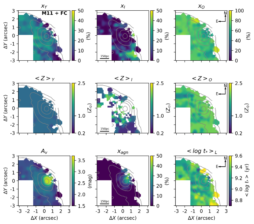
Figure 16: Same as Fig. 14 for M11+FC.

The maps of the recovered properties from the three distinct bases are shown in Fig. 14, Fig. 15 and Fig. 16 at the Appendix A. These figures show the maps for $x_{Y}$, $x_{I}$, $x_{O}$, $x_{agn}$, $A_{V}$, the light-weighted stellar mean age $\langle log\ t_{*}\rangle$ defined as:

$$\langle log\ t_{*}\rangle=\frac{\sum_{j=1}^{N_{*}}x_{j}log(t_{j})}{\sum_{j=1}^{N_{*}}x_{j}}$$ (2)

where $x_{j}$ are the elements of the population vector $\vec{x}$, i.e. the fraction contribution of each component to the total light, $t_{j}$ is the ages of $j$-th component, and $N_{*}$ is the number of stellar spectra in the base (SSPs). The figures in Appendix A also shows the light-weighted stellar mean metallicity $\langle{\rm Z}\rangle$ for each reduced population vector component $x_{Y}$, $x_{I}$ and $x_{O}$, respectively $\langle{\rm Z}\rangle_{Y}$, $\langle{\rm Z}\rangle_{I}$ and $\langle{\rm Z}\rangle_{O}$, defined as:

$$\langle{\rm Z}\rangle=\frac{\sum_{j=t_{0}}^{t_{f}}x_{j}z_{j}}{\sum_{j=t_{0}}^{t_{f}}x_{j}}$$ (3)

where $t_{0}$ and $t_{f}$ are respectively the lower and upper age limit of the reduced population vector components as defined in the previous section.

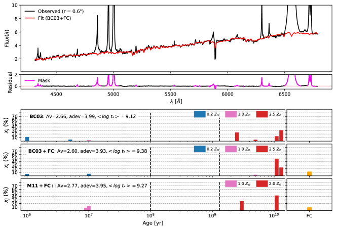
Figure 2: Example of stellar population synthesis fit. Top: Observed (black) and synthetic (red) spectra both in units of 10^-15 $\rm erg\,s^{-1}\,cm^{-2}\,\textup{\AA}^{-1}$in a spaxel at radius equal to $0\aas@@fstack{\prime\prime}6$. Middle: Residual between the observed and synthetic spectra, masked emission lines are shown in purple. Bottom: Age/metallicity and FC decomposition for the three synthesis, BC03, BC03+FC and M11+FC. The dashed lines show the division between $x_{Y}$, $x_{I}$ and $x_{O}$ SSPs.

The upper panel of Fig. 2 shows an example fit for a spaxel at $r=0\aas@@fstack{\prime\prime}6$, the residuals between the observed and the fitted spectra and the emission line mask. At the bottom panels the age/metallicity/FC decomposition for the three syntheses are shown as an example of the small differences resulting from the change of spectral base (see subsection 3.3 and subsection 3.4).

In Fig. 3 we show the radial profiles of $x_{Y}$, $x_{I}$, $x_{O}$, $x_{agn}$ and $\langle log\ t_{*}\rangle$, in bins of 0$\aas@@fstack{\prime\prime}$45 ($\approx$ 70 pc), with points representing the median, and the coloured region represents the 25 and 75 percentiles of the azimuthal distribution for the given radial bin. In Fig. 4 we show the values of $\langle{\rm Z}\rangle$ for each one of the bases integrated over the entire FoV.

In general terms the presence of a large contribution of old metal-rich SSPs and a smaller, but significant, contribution of young metal-poor stars seems to be independent of the presence of an FC component, or the change of model/library. The detailed analyses of the differences caused by the distinct spectral bases available to the code will be better explored in the sections below.

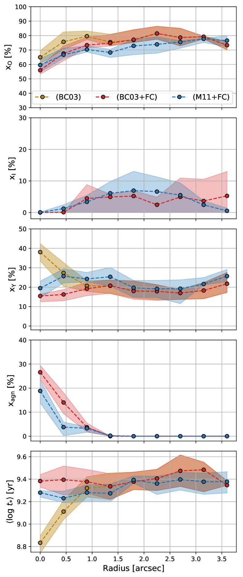
Figure 3: Radial profiles of the recovered properties for BC03 (gold), BC03+FC (red) and M11+FC (blue) in bins of $0\aas@@fstack{\prime\prime}45$ ($\sim$ 70 pc). From top to bottom: Per cent contribution to the total light from young ($x_{O}$), intermediate ($x_{I}$) and old ($x_{Y}$) SSPs, from the FC ($x_{agn}$) and the light-weighed mean stellar age ($\langle log\ t_{*}\rangle$). $x_{agn}$ is null for BC03 by definition. The $x_{I}$ values for BC03 are not shown, however they are exactly the same as BC03+FC.

3.3 The FC Component Usage: Comparing BC03 and BC03+FC

As shown by Fig. 3, the differences in the BC03 and BC03+FC synthesis are seen only at the inner spaxels and are linked to the presence of the FC component in the spectral base. For the external spaxels ($r>1\aas@@fstack{\prime\prime}1$), where only BC03 stellar components are used in both synthesis, the recovered properties are identical, as one would expect. In the external spaxels, the $x_{O}$ values range between 75 per cent and 85 per cent, with all spaxels having super-solar mean metallicity, $\langle{\rm Z}\rangle_{O}>1.5$ ${\rm Z_{\odot}}$, and the majority of them being close to the upper limit of the models, $\langle{\rm Z}\rangle_{O}\approx 2.5$ ${\rm Z_{\odot}}$. The $x_{Y}$ values are between 15 per cent and 25 per cent, with most spaxels having a sub-solar mean metallicity, $\langle{\rm Z}\rangle_{Y}\leq 1.0$ ${\rm Z_{\odot}}$, with a considerable portion of them at the lower limit of the model, i.e. $\langle{\rm Z}\rangle_{Y}=0.2$ ${\rm Z_{\odot}}$. Some properties are identical in all runs even at the inner spaxels, $A_{V}$ is very high in the innermost spaxels ($A_{V}>3$ mag) declining rapidly to $A_{V}\approx 2.5$ mag and reaching 1.5 mag at the border spaxels ($A_{V}$ map shown at Appendix A). Similarly, the contribution from intermediate SSPs, $x_{I}$, is null at most spaxels and reaches a maximum value between 10 and 20 per cent in very few regions.

Comparing the inner spaxels of BC03 and BC03+FC, we see that the presence of an FC component in the base causes a decrease in $x_{O}$ by just a few per cent. Larger differences, however, are seen in the contribution from young stars, especially where an FC component is not available (BC03). In this case, there is a sharp increase in $x_{Y}$ from a steady 20 per cent at $r>1$″to more than 40 per cent at the centre. On the other hand, the (BC03+FC) base produces a roughly constant $x_{Y}$ at $r<1.0\arcsec$, while $x_{agn}$ increases from $\sim$0 per cent at 1.0″to $\sim$20 per cent in the innermost spaxels. This effect is caused by the above-mentioned degeneracy between an FC spectrum and a young-reddened SSP (Cid Fernandes et al., 2004; Cid Fernandes & González Delgado, 2010). As shown by Cardoso et al. (2017), fitting a spectrum that contains an AGN power law-like continuum with only stellar components causes the solution to have an excess of young populations, which leads to a drop in the $\langle log\ t_{*}\rangle$ (see the bottom panel of Fig. 3). Although such degeneracy can cast some doubts in the exact values of the $x_{Y}$ and $x_{agn}$ decomposition in BC03+FC, the fact that the solution at the centre has $x_{Y}$ values compatible with the ones of the external regions of the FoV, and that the FC component contribution follows a radial profile compatible with an unresolved source (i.e increasing from $x_{agn}\approx$ 0 per cent to $x_{agn}\approx$ 20 per cent at the continuum peak) is strong evidence in favour of the existence of an FC emission in NGC 2992.

3.4 Decomposition Stability: Comparing BC03/STELIB and M11/MILES

In this section we discuss differences in the recovered properties between BC03+FC and M11+FC bases and their derivations. We do not intend to make a detailed analysis of the models and its derivations, nor to suggest one is a better choice than the other for use with this type of data. Such discussions can be found in other studies, e.g. Baldwin et al. (2018); Ge et al. (2019). Instead, we merely want to test the stability of the inferred stellar properties with changes in models.

Besides the distinct stellar libraries used in these model libraries, they also employ different evolutionary prescriptions (see Conroy, 2013, for a review on stellar evolutionary models). BC03 is constructed using the isochrone synthesis approach, while M11 uses the fuel consumption theory. The treatment of the thermally pulsing asymptotic giant branch (TP-AGB) phase is also a major topic of disagreement between different models. For example, Dametto et al. (2019) found a relative excess of young populations and lack of intermediate-age components when Near-Infrared (NIR) stellar populations synthesis are performed with BC03 SSPs, favouring results achieved with the M11 models. Nevertheless, these effects are much more important when modelling stellar populations in the NIR, being significantly less relevant in the optical.

Both $x_{agn}$ and $A_{V}$ are very similar to those obtained with BC03+FC, but the population vectors have notable differences. For instance, $x_{O}$ values for M11+FC are systematically lower by $\sim$5 to 10 per cent than those recovered with BC03+FC, while at the same time both $x_{Y}$ and $x_{I}$ are conversely higher for M11+FC. Given the increase of both $x_{Y}$ and $x_{I}$ and the decrease in $x_{O}$, the light-weighted mean stellar age $\langle log\ t_{*}\rangle$ for M11+FC is systematically lower than for BC03+FC by $\sim$ 0.5 to 0.1 dex, as show in the bottom panel of Fig. 3.

Although there are small differences in age decomposition, the metallicity general pattern seems to be maintained. As can be seen in Fig. 4, the old populations have a super-solar mean metallicity, close to the upper limit of the model ($1.5$ ${\rm Z_{\odot}}$ $<\langle{\rm Z}\rangle_{O}\ \leq 2.0$ ${\rm Z_{\odot}}$) and the young populations have a solar to sub-solar mean metallicity ($\langle{\rm Z}\rangle_{Y}\ \leq 1.0$ ${\rm Z_{\odot}}$), as shown in the middle panels of Fig. 4. However, while the values of $\langle{\rm Z}\rangle_{Y}$ in BC03+FC are mostly sub-solar ($\langle{\rm Z}\rangle_{Y}<1.0$ ${\rm Z_{\odot}}$) the values in M11+FC are all solar ($\langle{\rm Z}\rangle_{Y}=1.0$ ${\rm Z_{\odot}}$). This discrepancy is probably caused by the fact that the MILES library does not contain SSPs with a sub-solar metallicity younger than 55 Myr (see LABEL:table:SSPs). For instance, in the example of Fig. 2, while BC03 and BC03+FC recover its young populations as a combination of three SSPs with ages of 1 Myr, 5 Myr and 10 Myr, the two first with sub-solar metallicity ($Z=0.2$ ${\rm Z_{\odot}}$) and the later with solar metallicity ($Z=1.0$ ${\rm Z_{\odot}}$), the M11+FC recovers it as both 9 Myr and 10 yr solar metallicity SSPs, and the fitting code would not be able to fit such a young component with lower metallicity precisely because MILES library does not provide an SSPs with $Z=0.5$ ${\rm Z_{\odot}}$ younger than 55 Myr. Therefore, we can see these $\langle{\rm Z}\rangle_{Y}=1.0$ ${\rm Z_{\odot}}$ values in the synthesis using M11+FC base as an upper limit for the young population metallicity.

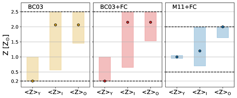
Figure 4: Values of $\langle{\rm Z}\rangle$ _Y, $\langle{\rm Z}\rangle$ _I and $\langle{\rm Z}\rangle$ _O integrated over the entire FoV for each base, from left to right, respectively, BC03, BC03+FC and M11+FC. Points are the median values, and the coloureds bars are the 25 and 75 percentiles. The dashed black lines show the metallicity limit for each of the models.

As mentioned, above, we do not claim any of the three syntheses to be the one that better describes the data. In fact, there are no significant differences in the adev parameters among the bases: adev values range from 3 per cent at the inner spaxels up to 8 per cent at larger radius. Recovered properties produced with the distinct models present the same general trend (see subsection 3.2). However, we argue the bases which include an FC component are more physically justified. Both the large decrease in $\langle log\ t_{*}\rangle$ in the inner spaxels, when this component is ignored, and the fact that the FC components fluxes have a spatial profile characteristic of a point-like source (FWHM $\approx$ $0\aas@@fstack{\prime\prime}8$, see Fig. 7) are strong evidence of the existence of an FC like emission in NGC 2992. It is worth mentioning even though we are not discussing results for the stellar kinematics, we have made sure all the three decompositions were kinematically consistent with each other, and no non-physical value was fitted to $v_{*}$, $\sigma_{*}$ parameters, which would cause an incorrect subtraction of the continuum used in emission line fitting procedures of the next sections.

4 GAS KINEMATICS

Emission line structure of the central regions of AGN is very complex, often possessing multiple velocity components along the line of sight (e.g. Villar-Martín et al., 2011; Veilleux et al., 2013; McElroy et al., 2015). For the type-1 and intermediate-type AGNs, the presence of both narrow and broad emission lines are seen; these emission lines are believed to come from two distinct parts of the AGN. The first is named the "Broad Line Region" (BLR). Its typical size, as deduced from the broad line variability, is 10-100 light-days, therefore it is spatially unresolved by current observations, meaning that its spatial profile is the same as the point spread function (PSF) of the observation. BLR emission is characterised by very broad (1000 $\rm km\,s^{-1}$< FWHM < 10000 $\rm km\,s^{-1}$) Balmer lines and the absence of forbidden lines (Peterson, 1997). In most cases, the line profiles strongly deviate from a Gaussian profile, e.g. NGC 1097 (Schimoia et al., 2015). The second region is the "Narrow Line Region" (NLR) which is much larger than the BLR since no clear variation of the narrow emission lines is observed in objects undergoing large variations of the AGN’s featureless continuum on timescales shorter than several years. The NLR is resolved by ground-based observations showing dimensions of 100-1000 pc in most nearby AGNs and up to several kpc’s in higher redshift quasars (Bennert et al., 2006; Sun et al., 2017; Storchi-Bergmann et al., 2018). The NLR emission is characterised by both permitted and forbidden lines with lower velocity dispersion (FWHM < 1000 $\rm km\,s^{-1}$), but still broader than emission lines of normal star forming galaxies. Even the NLR emission lines are some times not well fitted by a simple Gaussian profile, given the presence of multiple kinematical components in the line of sight, e.g. gaseous disk rotation, gas outflows and inflows (e.g. Zakamska et al., 2016; Schnorr-Müller et al., 2017).

4.1 Emission line fitting

In order to fit the emission lines in NGC 2992 we use the IFSCube package (Ruschel-Dutra, 2020). IFSCube is a python based software package designed to perform analysis tasks in data cubes of integral field spectroscopy, mainly focused on the fitting of spectral features, such as atomic lines. It allows for multiple combinations of Gaussian and Gauss-Hermite functions, with or without constraints to its parameters. Stellar continuum subtraction, as well as pseudo continuum fitting if necessary, are performed internally, and in this case, we used the residual spectra from the stellar population synthesis performed with starlight. Initial guesses for the parameters are set for the first spaxel, usually, the one with the highest $S/N$, and all subsequent spectra use the output of neighbouring successful fits as the initial guess.

When dealing with complex emission, the standard approach is to model the line profile with a combination of Gaussian functions. Visual inspection of our IFU shows distinct velocity components, evidenced by large asymmetries in the line profiles, are present in over one-third of the spectra in the FoV. As a result, we decided to model these components separately and to investigate whether they possessed any meaningful physical information, following previous works (e.g. Villar-Martín et al., 2011; McElroy et al., 2015; Fischer et al., 2018).

For every fitted emission line, we determined if the multi-component model was statistically justified, and not a better fit purely by virtue of the extra model parameters, by performing a series of f-tests. The f-test is a standard statistical test to gauge whether a higher order model is preferable to a simpler model when fitting a particular data set. We set the false rejection probability for the lower order model to 10^-5. The higher this threshold is set, the harder it is to justify a more complex model and the more likely it is to be over-fitting noise. The reader interested in more detailed analyses and a step-by-step deduction of the application of f-test in astrophysics emission line fitting is referred to Freund (1992) and statistical references therein.

As an Intermediate-type Seyfert nucleus, NGC 2992 presents both BLR and NLR emission. The BLR emission lines (H$\alpha$ and H$\beta$) are blended with some NLR emission lines (H$\alpha$, $[\text{N\,{ii}}]\lambda 6548$, $[\text{N\,{ii}}]\lambda 6583$ and H$\beta$), leading to degeneracies if both NLR and BLR emission lines are fitted, spaxel by spaxel, at the same time with all parameters free. Fortunately, the fact that the BLR is not resolved, i.e. its kinematics and its Balmer decrement (H$\alpha$/H$\beta$) can not vary spatially, can be used to decrease this degeneracy. Our chosen methodology consists on first fitting an integrated spectrum to fix the BLR emission line profile (kinematics and Balmer decrement), and later using this BLR spectrum as a fixed component, except for the flux, on the spatially resolved NLR fits.

We extracted a spectrum centred at the continuum peak, using a virtual aperture of $3\sigma=1\aas@@fstack{\prime\prime}1$ ($\sigma$ refers to the Gaussian point spread function). In this spectrum we fitted $[\text{N\,{ii}}]\lambda 6548$, $[\text{N\,{ii}}]\lambda 6583$, H$\alpha$ (both BLR and NLR) and H$\beta$ (both BLR and NLR), adding Gaussian components to the emission lines until the addition of a new component does not increase the fitting quality, as measured by the f-test described above. The final fit has shown that two Gaussians are necessary to fit each one of the BLR Balmer emission lines. This resulting profile, meaning the superposition of two Gaussian functions, hereafter called as BLR Component, can be seen in panel (1) of Fig. 5, and is characterised by a FWHM${}_{\rm BLR}=2010$ $\rm km\,s^{-1}$and a Balmer decrement of (H$\alpha$/H$\beta$)${}_{\rm BLR}=24.2$. These values are in considerable agreement with the ones fitted by Schnorr-Müller et al. (2016), FWHM${}_{\rm BLR}=2192$ $\rm km\,s^{-1}$and (H$\alpha$/H$\beta$)${}_{\rm BLR}=19.2$, considering these authors used three Gaussian functions to model the profile and the BLR of NGC 2992 has been shown to vary in a few years period (L. Trippe et al., 2008).

In order to resolve the kinematics of the NLR and obtain maps of emission line ratios, we fitted the following eight strongest emission lines present in the data cube: H$\beta$, $[\text{O\,{iii}}]\lambda 4959,\lambda 5007$, H$\alpha$, $[\text{N\,{ii}}]\lambda 6548,\lambda 6583$ and $[\text{S\,{ii}}]\lambda 6716,\lambda 6731$. Each emission line was modelled with a set of Gaussian functions. The central wavelength of the Gaussian functions was allowed to vary by up to $\pm$400 $\rm km\,s^{-1}$and the velocity dispersion up to 400 $\rm km\,s^{-1}$(FWHM $\approx 1000$ $\rm km\,s^{-1}$). We added one more set of Gaussians to the fit, meaning that each emission line is modelled by up to two Gaussian components. To reduce the number of free parameters, each set of Gaussians was required to have the same velocity and velocity dispersion (meaning their relative wavelengths were fixed), while their fluxes were allowed to vary. The reason for this is each component represents a kinematically distinct part of the gas, meaning that they may have different ionisation states determined by their relative fluxes. This means that, for example, the single-component set of Gaussians fit to the eight emission lines instead of having twenty four (eight lines $\times$ three parameters) free parameters, only had nine (a single velocity, $v$, and velocity dispersion, $\sigma$, amplitudes of H$\alpha$, H$\beta$, the two [S ii] and the stronger [N ii] and [O iii], while the amplitudes of the weaker [N ii] and [O iii] were set fixed as 1/3 of the stronger ones, as given by their Quantum Mechanics’ probabilities (hereafter we call $[\text{O\,{iii}}]\lambda 5007$ as [O iii], $[\text{N\,{ii}}]\lambda 6583$ as [N ii], and the $[\text{S\,{ii}}]\lambda 6716,\lambda 6731$ as [S ii]). As described in the previous paragraph, the BLR Component was also included in the fit with only the amplitude as free parameter.

To estimate the uncertainties in the parameters, we performed Monte Carlo simulations, in which Gaussian noise was added to the observed spectrum. One hundred iterations were performed and the estimated uncertainty in each parameter was derived from the standard deviation in all the iterations. The uncertainty maps are presented in Appendix B.

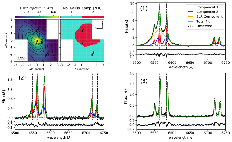
Figure 5: Top left: Map of the continuum emission at $\lambda$ = 5500 Å and map of the preferred number of Gaussian components to the [N ii] emission-lines. Top right and bottom: Examples of the H$\alpha$, $[\text{N\,{ii}}]\lambda 6548,\lambda 6583$ and $[\text{S\,{ii}}]\lambda 6716,\lambda 6930$ emission lines fitting and their residual in distinctly regions of the FoV marked in the maps. The vertical axis units in the panels showing the emission-line profiles are 10^-15 $\rm erg\,s^{-1}\,cm^{-2}\,\textup{\AA}^{-1}$and the dashed vertical lines show rest-frame wavelength of the lines.

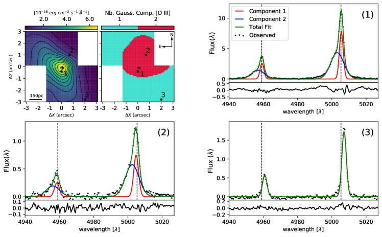
Figure 6: Same as Fig. 5 but for [O iii] emission lines.

We then applied the f-test to each one of the NLR emission lines, spaxel by spaxel, in order to assess if the simple model (single-Gaussian) is enough to fit the data or the more complex model (two Gaussians) is required. The f-test results in spatially contiguous regions of the required number of components for each emission line. The maps for [N ii] and [O iii] emission lines are shown in Fig. 5 and Fig. 6. The figures also show spectral and emission line fits in selected regions of the FoV.

The maps are not exactly equal for all emission lines, the size of the region in which two components are needed depends on the line S/N, therefore the size is maximum for [O iii] (Fig. 6) and H$\alpha$ (Fig. 11), a little bit smaller for [N ii] (Fig. 5) and the [S ii] doublets (not shown) and much smaller for the low S/N line, H$\beta$ (not shown). However, the general pattern is the same for all emission lines: the data are well fitted by a single-Gaussian in most of the FoV, but in a region, from the nucleus to the end of the FoV in the northwest (NW) direction two Gaussians are needed.

As can be seen in both figures, for those spaxels in which the emission lines are well behaved and symmetric, a single-Gaussian function, which we will call Component 1, is enough to fit the data. However, in the spaxels where two components were statistically significant, the profiles show an asymmetry in the form of a blueshifted wing (see panels (1) and (2) in Fig. 5 and Fig. 6) requiring the addition of a second Gaussian, which we will call Component 2.

In Fig. 7 we show the spatial and radial profile of the BLR Component. As expected for an unresolved structure, this component is detected just in the innermost spaxels, with a spatial distribution of a point-like source, equal to that of the stars in the acquisition image (FWHM $\approx 0\aas@@fstack{\prime\prime}8$, see section 2); at radii larger than $3\sigma$ (1.1 arcsec) it is almost undetectable.

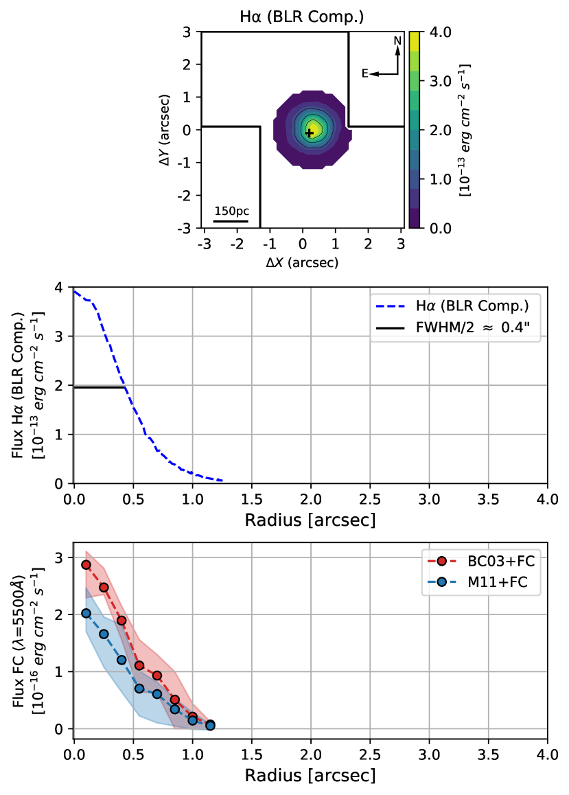
Figure 7: Top: Spatial distribution of the BLR Component. Middle: Radial projection of the BLR Component profile, vertical axis units of 10^-13 $\rm erg\,s^{-1}\,cm^{-2}$. Both show the point-like source emission of the BLR, with a FWHM $\approx 0\aas@@fstack{\prime\prime}8$ given by the spatial resolution of the observation. Bottom: Radial projection of the FC components fluxes (see section 3), also presenting a point-like source emission.

4.2 Rotational and Non-Rotational Components in the NLR

Let us now discuss the spatially resolved properties of the NLR Components 1 and 2 and their possible physical interpretation. Component 1 is present in the entire FoV. In the top panels of Fig. 8 we show, from left to right, [O iii] flux, velocity dispersion ($\sigma$), already corrected by instrumental dispersion. In the middle left panel, we present the radial velocity ($v$). We show the [O iii] flux as an example of the morphology of this component, which is similar to the continuum morphology, with the peak of the emission shifted by only $\sim 0\aas@@fstack{\prime\prime}2$ to southwest (SW), with a steep decrease (up to 2 $dex$) towards the dust lane region. The $\sigma$ values range from 50-100 $\rm km\,s^{-1}$and show a very disturbed pattern. The $v$ map shows values from -130 to 120 $\rm km\,s^{-1}$and although it presents some disturbance, a rotation pattern is clearly discernible, with the SW portion receding and the northeastern (NE) approaching. We have considered the west side of the galaxy is the near one, following the literature (e.g. Marquez et al., 1998; Veilleux et al., 2001); this explains why the emission is seen mainly to the east and less to the west where it is attenuated by the dust lane in the line-of-sight.

In order to quantify how much the velocity field deviates from a pure rotation and to derive both the major axis PA and the inclination of disk we fit the Bertola et al. (1991) model. The model assumes a spherical potential with pure circular orbits, in which the observed radial velocity at a position ($R$, $\psi$) in the plane of the sky given by the relation:

$$v(R,\psi)=v_{\rm sys}+\\ \frac{AR\cos(\psi-\psi_{0})\sin\theta\cos^{p}i}{\left\{R^{2}\left[\sin^{2}(\psi-\psi_{0})+\cos^{2}(\psi-\psi_{0})\right]+c_{0}^{2}cos^{2}i\right\}^{p/2}}$$ (4)

where $v_{sys}$ is the systemic velocity, $i$ the inclination of the disk (with $i$ = 0 for a face-on disk), $A$ is the amplitude of the curve, c₀ is the concentration parameter and $\psi_{0}$ the line of nodes PA. The parameter $p$ defines the form of the rotation curve, varying in the range between 1 (logarithm potential) and 1.5 (Keplerian potential). To avoid the degeneracy between the parameters, we restricted the disk inclination to have values of $i$ = 70 $\pm$ 10 (based on Duc et al., 2000, photometric analyses) and we assumed the kinematical centre to be co-spatial with the peak of the continuum emission. A Levenberg-Marquardt least-squares minimisation was performed to determine the best fitting parameters and the uncertainties were obtained by making one hundred Monte Carlo iterations. We show the best parameters and their uncertainties in Table 2.

Table 2: Best Fitting Parameters Bertola et al. (1991) Model.

Parameters	Values
$v_{sys}$	2345 $\pm$ 5 [ $\rm km\,s^{-1}$]
$A$	132 $\pm$ 4 [ $\rm km\,s^{-1}$]
$p$	1a
$c_{0}$	3.5 $\pm$ 0.1 [arcsec]
$\psi_{0}$	$32^{\circ}\pm 1^{\circ}$
$i$	$70^{\circ}\pm 1^{\circ}$

^a In the model the parameters $p$ is allowed to vary between 1 and 1.5, the fitted value was equals to 1 in all the Monte Carlo iterations.

The PA of the line of nodes was measured as 32$\pm$1^∘, in agreement with previous values from the literature: PA = 32^∘ (Veilleux et al., 2001, hereafter V01), PA= 30^∘ (Marquez et al., 1998, hereafter M98). V_sys and i are also in reasonable agreement with other studies of the galaxy: V01 found, respectively, $2335\pm 20$ $\rm km\,s^{-1}$and 68^∘, while M98 found 2330 $\rm km\,s^{-1}$and 70^∘. The velocity field amplitude (A = 132$\pm$4 $\rm km\,s^{-1}$), though, is much lower than the ones found by both V01 and M98 (225$\pm$20 $\rm km\,s^{-1}$and 250 $\rm km\,s^{-1}$). This discrepancy is probably due to the fact that both have used long-slit data in their studies, therefore being able to map the velocity field up to several kpc. Thus having a better constraint in the behaviour of the field at a larger radius, while our data can only recover the internal portion of the velocity field.

The modelled velocity field is shown in the middle right panel of Fig. 8, and the residuals between the observed field and model are shown in the bottom left panel of the same figure. The uncertainty map for the Comp. 1 $v$ field, as measured by the Monte Carlo simulations described in the subsection 4.1, is shown in the bottom right of Fig. 8. While most of the field is well represented by the disk rotation model ($\left|v-v_{Model}\right|<20$ $\rm km\,s^{-1}$), there is one region at the eastern border with residuals up to 40 $\rm km\,s^{-1}$. Since the maximum uncertainty in $v$ is 15 $\rm km\,s^{-1}$, this deviation from pure rotation is probably real. The same seems to be true for the $\sigma$ field, shown in Fig. 9. The uncertainties in the Component 1 $\sigma$ are of $\sim$5 $\rm km\,s^{-1}$in the central region, and up to 15 $\rm km\,s^{-1}$at the borders, as shown in Fig. 17. Therefore, the lack of structure in the $\sigma$ map is, in fact, real and not due to observational artefacts.

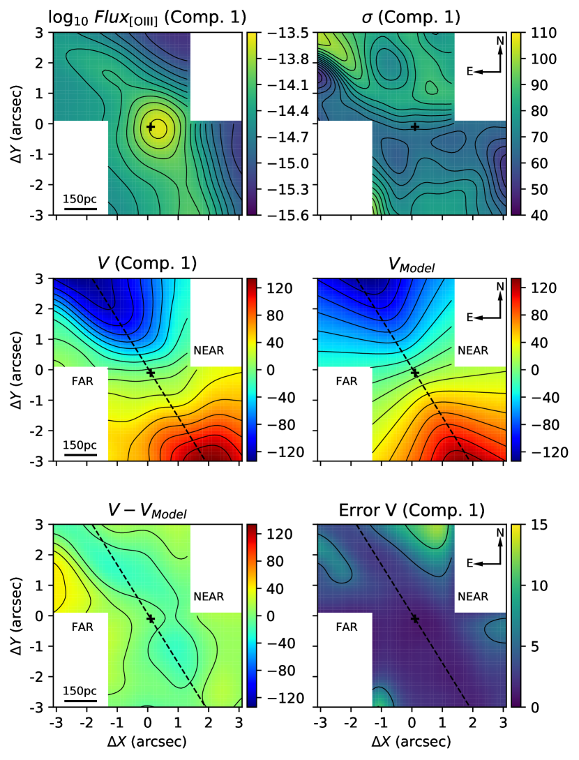
Figure 8: Component 1 properties. Top left: Log₁₀ Flux [O iii] $\lambda$5007 ( $\rm erg\,s^{-1}\,cm^{-2}$). Top right: Velocity dispersion $\sigma$ ( $\rm km\,s^{-1}$). Middle left: Radial velocity $v$ ( $\rm km\,s^{-1}$). Middle right: Modelled radial velocity ( $\rm km\,s^{-1}$), from the Bertola et al. (1991) rotation model fitting. Bottom left: Residual between the measured and the modelled velocity field. Bottom right: Uncertainties in the radial velocity $v$ ( $\rm km\,s^{-1}$). Black cross is the continuum peak and the dashed black line is the fitted major axis PA.

These types of disturbances, in the both $v$ and $\sigma$, are predicted by simulations (Kronberger et al., 2007; Bois et al., 2011) and observed (Torres-Flores et al., 2014; Hung et al., 2016; Bloom et al., 2018) in galaxies which are, or recently were, undergoing merging processes, as is the case of NGC 2992, and are attributed to perturbations in the gravitational potential due to tidal forces. In Paper II we will investigate whether these disturbances are also present in the velocity field of NGC 2993.

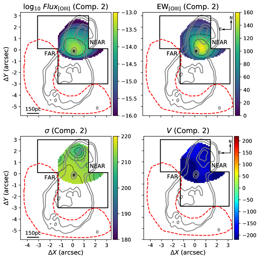
Figure 9: Component 2 properties. Top left: Log₁₀ Flux [O iii] $\lambda$5007 ( $\rm erg\,s^{-1}\,cm^{-2}$). Top right: Equivalent Width of [O iii] $\lambda$5007 (Å). Bottom left: Velocity dispersion, $\sigma$ ( $\rm km\,s^{-1}$). Bottom right: Radial velocity, $v$ ( $\rm km\,s^{-1}$). Solid black lines represent our FoV. Black cross is the continuum peak. Grey contours are the 6cm radio emission (Ulvestad & Wilson, 1984). Red dashed line is the contour of the redshifted structure found by García-Lorenzo et al. (2001), at the farthest part of the radio emission major loop, taken from Fig. 9 of their paper.

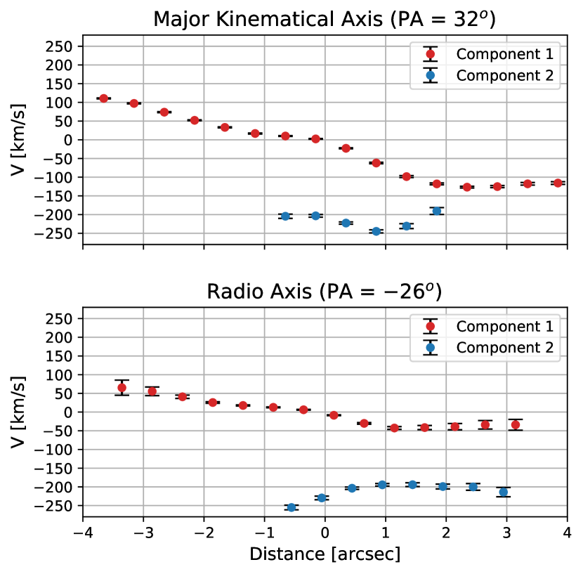
Figure 10: Position-Velocity plot in virtual slits with 0$\aas@@fstack{\prime\prime}$4 width. In the top panel the slit is at the PA of the major kinematical axis, in the bottom the slit is at the PA of 8-shaped radio emission major axis. Points are the measured velocity values, and the error bars are the uncertainties in the velocities. Red points are the velocities of Component 1 and blue points the Component 2 ones.

The fainter component of the NLR (Component 2) is detected in a smaller region, originating near the continuum peak and extending towards the NW. For the brightest line, $[\text{O\,{iii}}]\lambda 5007$, the emission extends up to $\sim$ 3″, as shown by both the flux map, top left panel of Fig. 9 and the P-V plot in Fig. 10. In Fig. 9, we show the maps of equivalent width (EW) of [O iii], $\sigma$ and $v$ for the Component 2. The $v$ map shows only blueshifted velocities, with values ranging from -250 to -200 $\rm km\,s^{-1}$. The velocity dispersion is higher than that of Comp. 1, ranging from 200 to 215 $\rm km\,s^{-1}$. We also show in all the panels, the contours of the 8-shaped region detected in the 6 cm radio emission (in grey) in which the smaller loop seems to be co-spatial with Component 2.

The position-velocity plot along the major kinematical axis (PA = 32^∘) and the major axis of the Radio emission (PA = -26^∘) of NGC 2992 are shown in Fig. 10. It is clear that while Comp. 1 has a rotational pattern, Comp. 2 deviates considerably from this pattern. Considering:

• Component 2 is not following the galaxy’s rotation;

• It is co-spatial with the radio emission;

• It has higher velocity dispersion values than those of Comp. 1, $\sigma>$ 200 $\rm km\,s^{-1}$;

• It has blueshifted velocities in the near side of the galaxy;

we are led to the conclusion that it is tracing a radio-jet driven gas outflow since all these are well-known characteristics of this type of phenomena. In fact, this ionised gas outflow was already reported by other IFU studies, e.g. García-Lorenzo et al. (2001), Friedrich et al. (2010) and Mingozzi et al. (2019). Particularly, García-Lorenzo et al. (2001) interpreted this blueshifted structure as the interaction of the minor loop of the radio-jet with the interstellar medium (ISM). García-Lorenzo et al. (2001) also found a similar, however redshifted, structure in the far side of the galaxy, co-spatial with the farthest part of the radio emission major loop, which is mostly not visible in our FoV. We have extracted the contours of this structure from Figure 9 of their paper and show it as the red dashed line in Fig. 9. This finding supports the scenario in which a bipolar over-pressure relativistic plasma is expanding, accelerating and compressing the ISM gas in its path (Chapman et al., 2000). Interestingly, the only portion of this structure which falls within our FoV is co-spatial with the largest velocity residuals seen in figure Fig. 8. Although our statistical analysis does not indicate the necessity of a separate component, the large residuals clearly indicate a perturbation in the velocity field.

A very similar geometry was found by Riffel & Storchi-Bergmann (2011) in the galaxy Mrk 1157, in which non-rotational blueshifted and redshifted structures are present and co-spatial to the two loops of a very similar nuclear 8-shaped radio emission. The authors also interpreted these structures as the effect of the expanding radio-emitting gas into the ionised ISM.

4.3 Outflow Properties

If we consider Component 2 as ionised outflowing gas, we can measure its properties such as mass, mass outflow rate and kinetic power. We followed the prescriptions described in Lena et al. (2015), in which a biconical outflow geometry is assumed, even though in our case we can see only one of the cones.

The mass outflow rate can be estimated as the ratio between the mass of the outflowing gas and the dynamical time (time for the gas to reach the present distance from the nucleus), M_g/t_d. The mass of the gas in outflow (Component 2) is estimated as:

$$M_{g}=n_{e}m_{p}Vf$$ (5)

where $m_{p}$ is the proton mass, $n_{e}$ and $V$ are the electron density and the volume of the region where the component is detected, $f$ is the filling factor. The filling factor and volume are eliminated by combining Equation 5 with the following expression for the H$\alpha$ luminosity:

$$L(H\alpha)\approx fn_{e}^{2}\,j_{H\alpha}\,V$$ (6)

with $j_{H\alpha}=3.534\times 10^{-25}$ erg cm³ s^-1 at $T=10000$K (Osterbrock & Ferland, 2006). Therefore, the gas mass can be written as:

$$M_{g}=\frac{m_{p}L(H\alpha)}{n_{e}j_{H\alpha}}$$ (7)

Our estimates for $n_{e}$ are based on the flux ratio between [S ii] lines, as described in Appendix C. Please note the $L(H\alpha)$ used here is based on the flux of Comp. 2 H$\alpha$ emission only, corrected by extinction as described in Appendix C. The spatially resolved $L(H\alpha)$ and M_g (i.e. gas mass surface density, $\Sigma_{\rm g}$) are shown in Fig. 11.

Figure 11: Left: Logarithm of Component 2 dereddened H$\alpha$ luminosity in erg s^-1. Right: Logarithm of Component 2 surface mass density in units of ${\rm M_{\odot}}$ ($0\aas@@fstack{\prime\prime}1$)^-2. Black cross is the peak of the continuum emission.

The integrated gas mass is $M_{g}=3.6\pm 0.6\times 10^{6}{\rm M_{\odot}}$. The t_d was estimated as the ratio between the maximum extension of the outflow $\sim 3\,\,{\rm arcsec}\approx 450\,\,{\rm pc}$ (see Fig. 10) to its mean velocity, $\left\langle v_{out}\right\rangle\approx 210$ $\rm km\,s^{-1}$, which gives t${}_{\rm d}\approx 2.2\times 10^{6}\,\,{\rm yr}$. Combining these values we estimated an outflow mass rate of $\dot{M}_{out}$ $\approx$ 1.6 $\pm$ 0.6 ${\rm M_{\odot}}$.

We also estimated the outflow kinetic power as:

$$\dot{E}_{out}=\frac{\dot{M}_{out}v_{out}^{2}}{2}$$ (8)

where $v_{out}$ is the radial velocity of Component 2 (Fig. 9). Integrating the entire outflow we obtained a total outflow kinetic power $\dot{E}_{out}\approx 2.2\pm 0.3\times 10^{40}\,\,{\rm erg\,s^{-1}}$. In subsection 6.3, we compare these values with the ones found in the literature and those expected by outflow-AGN relations.

5 Ionisation Mechanisms

Figure 12: Top: [N ii]/H$\alpha$ vs. [O iii]/H$\beta$ and [S ii]/H$\alpha$ vs. [O iii]/H$\beta$ BPT diagrams; grey countours are galaxies from the SDSS main galaxy sample. red points are the spaxel of NGC 2992. Colored markers are the selected regions of NGC 2992, as shown in the bottom panels, representing: red (Region A), blue (B), green (C), pink (D) and cyan (E). Middle: Zoomed BPT diagrams with shock+precursor grid models as measured with MAPPINGS V code (Sutherland et al., 2018); the $\vec{B}$ indicates increasing magnetic field of the model (from 0.01 to 4 $\mu$G); the black numbers indicates the velocities of the shocks, ranging from 300 to 900 $\rm km\,s^{-1}$. Bottom: Respectively, from left to right, [O iii]/H$\beta$, [N ii]/H$\alpha$, and [S ii]/H$\alpha$ emission lines ratio maps; red circles show the selected regions shown in the upper panels. In BPT diagrams the grey crosses are the typical errors in the emission line ratios; the solid black lines are Kewley et al. (2001) theoretical upper limits for pure star forming galaxies. In the [N ii]/H$\alpha$ vs. [O iii]/H$\beta$ diagram the dashed black line represents Kauffmann et al. (2003) line which traces the upper boundary of the SDSS star formation sequence. In the [S ii]/H$\alpha$ vs. [O iii]/H$\beta$ diagram the dashed-dotted black line represents the empirical division between AGN like and low-ionisation nuclear emission-line region (LINER) (Kewley et al., 2006).

Given the presence of young stars discussed in section 3, X-ray (section 1) and BLR emission (section 4) which indicate AGN excitation, and the presence of radio emission that can drive shocks (Dopita, 2002; Allen et al., 2008), we used the [N ii]/H$\alpha$ vs. [O iii]/H$\beta$ and [S ii]/H$\alpha$ vs. [O iii]/H$\beta$ Baldwin et al. (1981, BPT) diagnostic diagrams to investigate which of these excitation mechanisms are dominant in the innermost region of the galaxy.

In the bottom panels of Fig. 12, we show the maps of [O iii]/H$\beta$, [N ii]/H$\alpha$ and [S ii]/H$\alpha$ line ratios for the entire line profile (by summing the kinematical components; we do that to increase the precision in the flux measurement and to avoid regions where a second component is detected in high S/N lines, like [O iii], but not detected in lower S/N ones, like H$\beta$.) We excluded the regions where uncertainties in the total flux, as shown in Appendix B, are higher than 30 per cent. The [O iii]/H$\beta$ shows a clear AGN signature, with its peak, up to [O iii]/H$\beta$ $\approx$ 25, at the centre of the FoV and decreasing radially down to [O iii]/H$\beta$ $\approx 2$ at SW corner of the FoV. The [N ii]/H$\alpha$ and [S ii]/H$\alpha$, however, do not show the same pattern: their maximum values are off-nuclear, and they do not present a radial decrease as in the [O iii]/H$\beta$ one. This indicates a lower energy mechanism (lower than an AGN, but higher than H ii regions) can be ionising the gas too. In fact, shock ionised regions are characterised by having smaller [O iii]/H$\beta$ ratios and larger [S ii] ([N ii])/H$\alpha$ than those ionised by AGN (Veilleux & Osterbrock, 1987; Kewley et al., 2006; Allen et al., 2008).

We selected limiting regions in the line ratio maps and shown it in the respectively BPT diagrams in the top panels of Fig. 12. We also show some division lines: the solid black curves on both diagnostic diagrams trace the Kewley et al. (2001) theoretical upper limit of regions ionised by pure star formation (K01 line). All spectra lying above the K01 line are dominated by ionisation mechanisms more energetic than star formation. Several excitation mechanisms can increase the collisional excitation rate, enhancing the ratios of the forbidden to recombination lines, among them energetic photons from a power law-like emission (AGN); shock excitation and evolved stellar populations (pos-AGB) can also produce line ratios along this branch of the diagram. The latter case does not apply to the nuclear region of NGC 2992 given that it requires EW(H$\alpha$) < 3 Å (Stasinska et al., 2008; Cid Fernandes et al., 2011) and our entire FoV has EW(H$\alpha$) > 10 Å. We also show the dashed black curve on the [N ii]/H$\alpha$ vs. [O iii]/H$\beta$ diagnostic diagram: the Kauffmann et al. (2003) empirical classification line (Ka03 line), which traces the upper boundary of the Sloan Digital Sky Survey Strauss et al. (SDSS 2002) star formation sequence. All spectra lying below the Ka03 line are dominated by star formation. The dashed-dotted black curve on the [S ii]/H$\alpha$ vs. [O iii]/H$\beta$ diagnostic diagram traces the Kewley et al. (2006) empirical classification line (K06 line), which separates high ionisation spectra associated with Seyfert (AGN) and other intermediary ionisation mechanisms including shock excitation. We also show as grey points in the top BPT diagrams a collection of single-fibre emission line measurement from SDSS main galaxy sample by Kewley et al. (2006).

Region A is the peak of the [O iii]/H$\beta$ map, it shows clear AGN-like ratios, with an upper [O iii]/H$\beta$ value higher than any SDSS AGN, which corresponds to a 3″diameter aperture, and therefore has a diluted AGN/host-galaxy emission line ratio. Region B has the lowest value in all the maps; it lies below K01, showing the radial decrease in the AGN contribution to the emission lines and significant contributions from both star formation and AGN excitation. Regions C, D, and E display the highest values in the [S ii]/H$\alpha$ and [N ii]/H$\alpha$ maps; however, they have lower [O iii]/H$\beta$ values than region A. Region E, in fact, crosses the K06 line in the [S ii]/H$\alpha$ diagram, which again indicates the presence of another ionisation mechanism.

In order to search for an explanation to the increase in this intermediary ionisation energy lines ([N ii] and [S ii]) we used the MAPPINGS V shock models by Sutherland et al. (2018). We explored the parameter space in the pure shock and shock+precursor grids of the models. None of the pure shock models could explain these line ratios, given the high [O iii]/H$\beta$ values. However shock+precursor (Shock ionisation in a medium already ionised by power-law like emission) with shock velocities between 300 $\rm km\,s^{-1}$and 900 $\rm km\,s^{-1}$and magnetic field ($\vec{\rm B}$) between 0.01$\mu$G and 4$\mu$G, with a two-solar metallicity and a pre-shock density of 1 cm^-3, successfully reproduce the line ratios of regions C, D and E. In the middle panels of Fig. 12 we show the grid models in these shock velocity and magnetic field ranges superimposed with the emission line ratios of the regions. The shocks in NGC 2992 have been extensively studied by Allen et al. (1999), who conclude that shocks are the predominant ionisation mechanism in the extended NLR cones at a distance of several kpc from the nucleus.

We can conclude that a more simple Starburst-AGN mixture (e.g. Davies et al., 2014a, b; D’Agostino et al., 2018) in which the maximum values of all [O iii]/H$\beta$, [N ii]/H$\alpha$ and [S ii]/H$\alpha$ are located in the innermost spaxel (location of the AGN), and all decrease radially towards the H ii ionisation region of the BPT in a straight line (see for example figure 1 in Davies et al., 2014b), cannot describe the ionisation at the circumnuclear region of NGC 2992. Instead, a more complex Starburst-AGN-Shocks mixture is responsible for its ionisation. However, the very high values of [O iii]/H$\beta$ indicate the most important among these three mechanisms is AGN ionisation, at least in the innermost portion (see further discussion in subsection 6.4).

6 DISCUSSION

6.1 Interaction-Driven Circumnuclear Star formation

In general terms, the stellar population synthesis discussed in section 3 shows that stellar content in the inner 1.1 kpc of NGC 2992 is mainly composed by an old metal-rich population, with a smaller but considerable contribution from young metal-poor stars. The presence of the latter is supported by other studies, for instance, using the Bica & Alloin (1986) base of star clusters for stellar population synthesis, Storchi Bergmann et al. (1990) found a predominance of old stellar populations (10¹⁰ yr) and a small contribution of at least 5 per cent by recent star formation in the inner $5\arcsec$. Moreover, Friedrich et al. (2010) find that 10-20 per cent of the IR flux is attributable to a starburst, based on the emission from polycyclic aromatic hydrocarbon (PAH) molecules. Additionally, these authors estimate the starburst to have occurred between 40-50 Myr, based on the equivalent width of the Br$\gamma$ line.

Major merger processes are known to be responsible for gas inflow towards the central regions of galaxies enhancing circumnuclear star formation and possibly triggering nuclear activity. Merger galaxies have an increase in the SFR, mainly at the nuclear regions (Ellison et al., 2013; Pan et al., 2019). Thus, these sources have younger nuclear populations than those found in isolated galaxies, in which most of their recent formed stars are concentrated at the spiral arms. Moreover, major mergers are also able to modify the metallicity gradients of galaxies (Barrera-Ballesteros et al., 2015). Galaxy simulations show that the gas, originally located at external portions of the isolated galaxy (metal-poor regions), moves towards internal regions (metal-rich regions) of the companion galaxy during the encounter and is capable of cooling and forming stars.. Such processes are able to explain both the increase in the SFR and the modifications in the metallicity gradient (Dalcanton, 2007; Torrey et al., 2012; Sillero et al., 2017). In fact, the pericentre passage between NGC 2992 and its companion NGC 2993 is estimated to have occurred $\sim$ 100 Myr ago (Duc et al., 2000). Thus, a possible scenario is that metal-poor gas inflow has led to interaction-driven circumnuclear star formation which can explain the presence of such young metal-poor stellar population in the nucleus. Such inflows could also be responsible for triggering NGC 2992’s nuclear activity, a scenario which will be further explored using numerical simulations in Paper III.

6.2 Feeding vs Feedback

We can compare the mass outflow rate, estimated in subsection 4.3, with the accretion rate necessary to power the AGN at the nucleus of NGC 2992, calculated as follows:

$$\dot{M}_{\rm BH}=\frac{L_{bol}}{c^{2}\eta}$$ (9)

where $\eta$ is the mass-energy conversion efficiency, which for Seyfert galaxies is usually assumed to be $\eta=0.1$ (Frank et al., 2002), $L_{bol}$ is the bolometric luminosity of the AGN, and $c$ is the speed of light. To measure $L_{bol}$ we applied the bolometric correction by Marconi et al. (2004) on the most recent X-ray luminosity measurement of NGC 2992 made by Marinucci et al. (2018). The author used a 2015 NuSTAR observation and obtained an absorption corrected 2-10 Kev Luminosity of $7.6\pm 0.1\times 10^{42}\,\,{\rm ergs^{-1}}$ that translates to $L_{bol}=9.1\pm 0.2\times 10^{43}\,\,{\rm ergs^{-1}}$. We use these values to derive an accretion rate of $\dot{M}_{\rm BH}\approx 0.02\,\,{\rm M_{\odot}}yr^{-1}$.

The nuclear accretion rate is two orders of magnitude smaller than the mass outflow rate ($\dot{M}_{out}$ $\approx$ 1.6 $\pm$ 0.6 ${\rm M_{\odot}}$ yr^-1, see subsection 4.3). This implies that most of the outflowing gas does not originate in the AGN, but in the surrounding ISM, and this result supports the scenario in which the plasma bubbles (radio loops) are expanding, pushing gas away from the nuclear region. However, the ratio between the kinetic power of this blueshifted outflow loop and the bolometric luminosity is $\sim 0.002$, which means only 0.2 per cent of the AGN radiative power is in this outflow. Many authors argue that such a low value is not enough to have the feedback effects expected by cosmological simulations (Springel et al., 2005; Silk & Mamon, 2012; Bullock & Boylan-Kolchin, 2017), stating that $\dot{E}_{out}$/$L_{bol}$ should be closer to 5 per cent or above in order to effectively suppress growth in the most massive galaxies. However, some models show that coupling efficiencies of $\dot{E}_{out}$/$L_{bol}$ $\approx$ 0.5 per cent (Hopkins & Elvis, 2010), and even 0.1 per cent (Costa et al., 2018) could successfully prevent star formation.

6.3 AGN-Wind Scaling Relations

Comparing our outflow measurements with those from the literature we noted ours results disagree with those presented in Müller-Sánchez et al. (2011), who reported $\dot{M}_{out}$ = 120 M_⊙ yr^-1 and $\dot{E}_{out}$ = 2.5$\times$10⁴² erg s^-1, both almost one hundred times greater than ours. We attribute this difference to two factors: i) they assumed the filling factor $f$ to be constant equal to 0.001, while we have measured the filling factor from L(H$\alpha$) and $n_{e}$ (see Equation 6). This assumption makes their M_g proportional to $n_{e}$, and not inversely proportional (as in Equation 7); ii) they assume an electronic density of $n_{e}$ = 5000 cm^-3, a value more than 5 times larger than the maximum value we measured in the nuclear region of the galaxy. These two factors combined explain their overestimation of both $\dot{M}_{out}$ and $\dot{E}_{out}$. We also argue these differences cannot be due to a larger coverage of the outflow by a larger field of view, in the sense of seeing the farthest part of the radio emission major loop and its redshifted outflow structure, given the authors have used the OSIRIS/VLT instrument, which has an even smaller FoV than GMOS.

We can compare our values to the properties of outflows found in other precious papers across the literature. In Fig. 11, we show the Fiore et al. (2017) compilation of a set of outflow energetics from various studies over the years spanning a large range of AGN luminosity ($L_{bol}$ $\geq 10^{44}$), which they use to establish AGN wind scaling relations, mass outflow rate and outflow power as a function of bolometric luminosity, together with several measurements of nearby galaxies from individual studies compiled by us from the literature or obtained by our collaborators: NGC 1068, NGC 3783, NGC 6814, NGC 7469 (Müller-Sánchez et al., 2011), NGC 4151 (Crenshaw et al., 2015), Mrk 573 (Revalski et al., 2018), Mrk 34 (Revalski et al., 2018), NGC 7582 (Riffel et al., 2009), Mrk 1066 (Riffel et al., 2010b), Mrk 1157 (Riffel & Storchi-Bergmann, 2011), Mrk 79 (Riffel et al., 2013a), NGC 5929 (Riffel et al., 2013b), NGC 5728 (Shimizu et al., 2019), and NGC 3081 (Schnorr-Müller et al., 2014), ESO 362-G18 (Humire et al., 2018), NGC 1386 (Lena et al., 2015), ESO 153-G20 (Soto-Pinto et al., 2019), 3C 33 (Couto et al., 2017), including NGC 2992 measurement by Müller-Sánchez et al. (2011). Although these estimates are made using different recipes, leading to differences between methods, they are generally similar to the one adopted here. Therefore, this comparison with the literature may be useful at least as an order of magnitude approximation.

As we can see, the overestimated previous measurement of NGC 2992’s outflow made this source to be an outlier in the Fiore et al. (2017) relations, while our values make the galaxy more likely to be explained by these relations. However, the other measurements in nearby Seyfert galaxies support the existence of a larger scatter of these relations, both in $\dot{E}_{out}$ and $\dot{M}_{out}$, at lower luminosities. To confirm whether this extension is valid or not, more detailed studies like this, mainly using IFU, are needed so that outflow properties can be properly and systematically measured, without assuming fixed values of $n_{e}$ and $f$.

Figure 13: Correlations between the mass outflow rate ($\dot{M}_{out}$, Top Panel) and kinetic outflow power ($\dot{E}_{out}$, Bottom Panel). Blue points are the data compiled by Fiore et al. (2017) and the black dashed lines show the best fit correlations for these points. Red Squares are the previous measurement of NGC 2992 by Müller-Sánchez et al. (2011), and green ones are the results of this work. Violet diamonds are compiled from various literature sources for more modest AGN luminosities.

6.4 Multiple Ionisation Mechanisms

In section 5 we showed that despite being dominated by AGN excitation, star formation and shocks cannot be excluded as ionisation mechanisms in the nuclear region of the galaxy. The existence of star formation ionisation in the nucleus is confirmed by Friedrich et al. (2010) IR emission line analyses, as mentioned in subsection 6.1. The presence of shocks is also supported by Allen et al. (1999) using long-slit spectroscopy. The authors also argue the dominance of shocks increases, compared to ionisation by the central source, at larger radius.

Galaxies undergoing rapid phases of evolution (through processes such as galaxy-galaxy interactions, gas outflows and radio jets) often have multiple ionisation mechanisms contributing to their optical line emission (e.g. Rich et al., 2011; Lanz et al., 2015; Rich et al., 2015; Davies et al., 2017). These multiple ionisation mechanisms are also in agreement with evolutionary scenarios in which gas inflows (driven either by secular mechanisms, like nuclear bars or nuclear spiral arms, or environmental ones, like minor and major mergers) triggers nuclear star formation and nuclear activity (feeding process) and then the active nucleus can drive both ionising photons from the accretion disk and radio jets (feedback process) that impacts the ISM physical conditions (Hopkins et al., 2008; Hopkins & Quataert, 2010).

7 SUMMARY AND CONCLUSIONS

We have analysed the stellar population, the ionisation mechanism and kinematics of the ionised gas in the inner $1.1\,\,{\rm kpc}$ of the interacting Seyfert galaxy NGC 2992, using optical spectra obtained with the GMOS integral field spectrograph on the Gemini South telescope, with a spatial resolution of $\approx 120\,\,{\rm pc}$ and spectral resolution $\approx 40\,\,{\rm km\,s^{-1}}$. The main results are:

• The stellar population in the nuclear region of the galaxy is mainly composed (60 per cent$\leq x_{O}\leq 80$ per cent) by an old (t > 1.4 Gyr) metal-rich ($\langle{\rm Z}\rangle_{O}\geq 2.0$ ${\rm Z_{\odot}}$) population with a smaller, but considerable contribution (10 per cent $\leq x_{Y}\leq 30$ per cent) of an young (t < 100 Myr) metal-poor ($\langle{\rm Z}\rangle_{Y}\leq 1.0$ ${\rm Z_{\odot}}$) population. A possible scenario is that metal-poor gas inflow during the pericentre passage of NGC 2993 has led to interaction-driven circumnuclear star formation, which can explain the presence of such young metal-poor stellar population in the nuclear region;

• The emission line analyses show the presence of both BLR and NLR emission, confirming its classification as an intermediate-type Seyfert galaxy. The BLR emission profile has a velocity dispersion of FWHM${}_{\rm BLR}=2010$ $\rm km\,s^{-1}$and a Balmer decrement of (H$\alpha$/H$\beta$)${}_{\rm BLR}=24.2$. The NLR presents two distinctly kinematical components: one that although disturbed is well fitted by a disk model, and therefore can be identified as gas in orbit in the galaxy disk, with radial velocities ranging from -130 to 130 $\rm km\,s^{-1}$; another that we interpreted as an outflow associated with the radio emission, with blueshifted velocities of $\sim$ 200 $\rm km\,s^{-1}$, a mass outflow rate of $\dot{M}_{out}$ $\approx$ 1.6 $\pm$ 0.6 ${\rm M_{\odot}}$ and a kinematic power of $\dot{E}_{out}$ $\approx$ 2.2 $\pm$ 0.3 $\times$ 10⁴⁰ erg s^-1;

• The BPT diagnostic diagrams show the galaxy posses multiple ionisation mechanisms: a mixture of AGN, star-formation and shocks, the former being the dominant one. The [O iii]/H$\beta$ ratio peaks at the innermost spaxels, and is located in the upper region of the BPT diagram. The lower values, located at the border of the FoV, decreases down to below the Kewley et al. (2001) line, showing an increase in the star-formation ionisation compared to the AGN ionisation at larger radius. Off-nuclear peaks in the [N ii]/H$\alpha$ and [S ii]/H$\alpha$ maps indicate the presence of another mechanism and are successfully explained by Sutherland et al. (2018) shock+precursor models.

DATA AVAILABILITY

The data underlying this article will be shared on reasonable request to the corresponding author.

Appendix A Stellar Populations Synthesis Maps

We show the maps of the recovered properties from three spatially resolved starlight synthesis we have performed, namely BC03, BC03+FC and M11+FC. The top panels show, from left to right, the per cent contribution to the total light for young, intermediate and old SSPs ($x_{Y}$, $x_{I}$ and $x_{O}$). In the middle panels the light-weighted mean stellar metallicity for the three age groups, from left to right, $\langle{\rm Z}\rangle_{Y},\langle{\rm Z}\rangle_{I}$ and $\langle{\rm Z}\rangle_{O}$. In the bottom panel the V-Band extinction ($A_{V}$), the per cent contribution to the total light from the FC component ($x_{agn}$) and the light-weighted mean stellar age, $\langle log\ t_{*}\rangle$, are shown, respectively, from left to right.

Figure 14: Maps of the recovered properties from the BC03 synthesis. Top: from left to right, percentage contribution to the total light from young, intermediate and old SSPs ($x_{Y}$, $x_{I}$ and $x_{O}$). Middle: from left to right, light-weighted mean stellar metallicity for the three SSP age groups, $\langle{\rm Z}\rangle_{Y},\langle{\rm Z}\rangle_{I}$ and $\langle{\rm Z}\rangle_{O}$. Bottom left: $A_{V}$ extinction parameter. Bottom middle: Featureless continuum (FC) component percentage contribution to the total light ($x_{agn}$). Bottom Right: Light-weighted mean stellar age, $\langle log\ t_{*}\rangle$. The grey contour in all the maps is the continuum emission, left panel of Fig. 1. The $x_{agn}$ is null in all points by definition, because there is no FC component in BC03 synthesis spectra base.

Figure 15: Same as Fig. 14for BC03+FC.

Appendix B Emission Line Fitting Uncertainties

We present here the uncertainties in the parameters of the emission lines fitting described in subsection 4.1. The uncertainties are the standard deviation over the one hundred Monte Carlo iterations. The uncertainties in the radial velocity (V) of Component 1 was already presented in Fig. 8. In Fig. 17 we show the uncertainties in the velocity dispersion ($\sigma$) of Component 1, the values are mostly smaller than 5 $\rm km\,s^{-1}$, reaching a maximum value of 15 $\rm km\,s^{-1}$.

In the top panel we also show the uncertainties of $v$ and $\sigma$ of Component 2, values are less than 10 $\rm km\,s^{-1}$in most the region, reaching up to 30 $\rm km\,s^{-1}$in a very small region, the $\sigma$ values are less then 10 $\rm km\,s^{-1}$in the peak of component emission and up to 30 $\rm km\,s^{-1}$in the borders of the detection region. In the middle and bottom panels the percentile uncertainties in the integrated flux (Component 1 + Component 2) of H$\beta$, [O iii] $\lambda$5007, H$\alpha$, [N ii] $\lambda$6583, and [S ii] $\lambda$6716,6731 are shown.

The H$\beta$ line uncertainties range from 10 per cent at the centre of the FoV, up to 45 per cent in the dust lane region. [O iii] and H$\alpha$ values range from less than 5 per cent up to 25 per cent at the dust lane region. [S ii] and [N ii] values range from less than 10 per cent up to 35 per cent at the dust lane region.

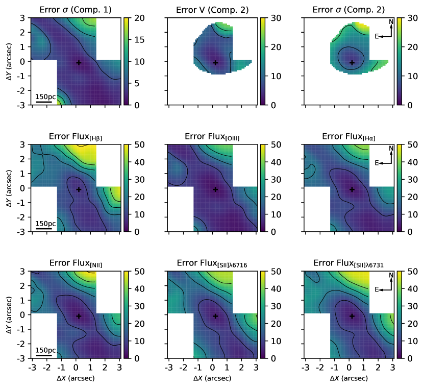
Figure 17: Emission line fitting uncertainties. Top: from right to left, velocity dispersion of Component 1 ( $\rm km\,s^{-1}$), radial velocity of Component 2 ( $\rm km\,s^{-1}$), velocity dispersion of Component 2 ( $\rm km\,s^{-1}$). Middle and Bottom: percentage uncertainties in the integrated flux (Component 1 + Component) of H$\beta$, [O iii] $\lambda$5007, H$\alpha$, [N ii] $\lambda$6583, and [S ii] $\lambda$6716,6731 (%). The black cross shows the peak of the continuum emission. Each contour in the maps means a 10% variation in the uncertainties.

Appendix C Nebular Extinction and Electron Density

In order to measure the extinction in the NLR, we adopt the Calzetti et al. (2000) extinction law, and assume the case B recombination and the intrinsic H$\alpha$/H$\beta$ value for the NLR (Osterbrock & Ferland, 2006), which combined leads to the following expression to the V-band extinction:

$$A_{\rm v}=7.95\times\log_{10}\left(\frac{\rm H\alpha/H\beta}{3.1}\right)$$ (10)

In order to improve the S/N and given the fact that H$\beta$ Component 2 is detected in a very small region, we used the integrated flux (Component 1 + Component 2) of the NLR H$\alpha$ and H$\beta$ lines. The $A_{\rm v}$ map is presented in the top left panel of Fig. 18, and its uncertainty in the bottom left panel. The $A_{\rm v}$ peak at $\sim$ 4.5 mag at the peak of the emission lines emission, and has values $>$ 3.5 mag in the dust lane portion of the FoV. However, this value may be even higher as the uncertainties are up to 2 mag in this region, caused by high impression on the H$\beta$ flux measurement, as seen in Fig. 17. Although the $A_{\rm v}$ are not the same in the continuum Appendix A and in the NLR, the spatial patterns are similar: the higher values are found the central spaxels and towards the dust lane, and the lower towards the SE direction.

The electron density ($n_{e}$) of the ionised gas in the NLR can be obtained from the ratio between the [S ii] lines, $[\text{S\,{ii}}]\lambda$6716/$\lambda$6731 (Osterbrock & Ferland, 2006). We applied the solution of the collisional equilibrium equations given by Proxauf et al. (2014) to obtain the $n_{e}$ values, as follows:

$$\log_{10}(n_{e}\ [cm^{3}]) =0.0543\tan(-3.0553R+2.8506)$$

$$+6.98-10.6905R+9.9186R^{2}-3.5442R^{3}$$ (11)

with R = $F_{6716}/F_{6731}$, the ratio between the [S ii] lines. The $n_{e}$ map in its uncertainties are presented, respectively, in the top right and bottom right panel of Fig. 18. The maximum value of $n_{e}$ is 950 $cm^{-3}$ reached at the peak of the emission lines, decreasing radially down to 100 $cm^{-3}$, another high ($\sim$ 800 $cm^{-3}$) density knot is present at the south of the nucleus. Both the values as well as the spatial profiles of both $A_{\rm v}$ and $n_{e}$ measured here are in agreement with the recent published analyses by Mingozzi et al. (2019) using MUSE instrument, see their Figures A1 and B1.

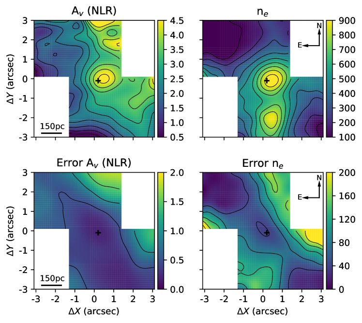
Figure 18: Top left and bottom left panels, shows, respectively the V-band extinction $A_{\rm v}$ map and its uncertainties, both in units of magnitudes. Top right and bottom right panel show, respectively, the electron density ($n_{e}$) and its uncertainties both in cm^-3 units. The black cross shows the peak of the continuum emission.

References

- Allen et al. (1999) Allen M. G., Dopita M. A., Tsvetanov Z. I., Sutherland R. S., 1999, ApJ, 511, 686
- Allen et al. (2008) Allen M. G., Groves B. A., Dopita M. A., Sutherland R. S., Kewley L. J., 2008, ApJS, 178, 20
- Alloin et al. (1979) Alloin D., Collin-Souffrin S., Joly M., Vigroux L., 1979, A&A, 78, 200
- Bacon et al. (2010) Bacon R., et al., 2010, in McLean I. S., Ramsay S. K., Takami H., eds, Society of Photo-Optical Instrumentation Engineers (SPIE) Conference Series Vol. 7735, Ground-based and Airborne Instrumentation for Astronomy III. p. 773508, doi:10.1117/12.856027
- Baldwin et al. (1981) Baldwin J. A., Phillips M. M., Terlevich R., 1981, PASP, 93, 5
- Baldwin et al. (2018) Baldwin C., McDermid R. M., Kuntschner H., Maraston C., Conroy C., 2018, MNRAS, 473, 4698
- Barrera-Ballesteros et al. (2015) Barrera-Ballesteros J. K., et al., 2015, A&A, 579, A45
- Begelman et al. (1984) Begelman M. C., Blandford R. D., Rees M. J., 1984, Reviews of Modern Physics, 56, 255
- Bennert et al. (2006) Bennert N., Jungwiert B., Komossa S., Haas M., Chini R., 2006, Astronomy & Astrophysics, 456, 953–966
- Bertola et al. (1991) Bertola F., Bettoni D., Danziger J., Sadler E., Sparke L., de Zeeuw T., 1991, ApJ, 373, 369
- Bica & Alloin (1986) Bica E., Alloin D., 1986, A&A, 162, 21
- Block (2011) Block A., 2011, Caelum-Observatory:NGC2992. http://www.caelumobservatory.com/gallery/n2992.shtml
- Bloom et al. (2018) Bloom J. V., et al., 2018, Monthly Notices of the Royal Astronomical Society, 476, 2339–2351
- Blumenthal & Barnes (2018) Blumenthal K. A., Barnes J. E., 2018, MNRAS, 479, 3952
- Bois et al. (2011) Bois M., et al., 2011, MNRAS, 416, 1654
- Bruzual & Charlot (2003) Bruzual G., Charlot S., 2003, MNRAS, 344, 1000
- Bullock & Boylan-Kolchin (2017) Bullock J. S., Boylan-Kolchin M., 2017, ARA&A, 55, 343
- Calzetti et al. (2000) Calzetti D., Armus L., Bohlin R. C., Kinney A. L., Koornneef J., Storchi-Bergmann T., 2000, ApJ, 533, 682
- Cappellari & Copin (2003) Cappellari M., Copin Y., 2003, MNRAS, 342, 345
- Cardelli et al. (1989) Cardelli J. A., Clayton G. C., Mathis J. S., 1989, ApJ, 345, 245
- Cardoso et al. (2017) Cardoso L. S. M., Gomes J. M., Papaderos P., 2017, A&A, 604, A99
- Chabrier (2003) Chabrier G., 2003, PASP, 115, 763
- Chapman et al. (2000) Chapman S. C., Morris S. L., Alonso-Herrero A., Falcke H., 2000, MNRAS, 314, 263
- Chen et al. (2010) Chen X. Y., Liang Y. C., Hammer F., Prugniel P., Zhong G. H., Rodrigues M., Zhao Y. H., Flores H., 2010, Astronomy and Astrophysics, 515, A101
- Cid Fernandes (2018) Cid Fernandes R., 2018, MNRAS, 480, 4480
- Cid Fernandes & González Delgado (2010) Cid Fernandes R., González Delgado R. M., 2010, Monthly Notices of the Royal Astronomical Society, 403, 780
- Cid Fernandes et al. (2004) Cid Fernandes R., Gu Q., Melnick J., Terlevich E., Terlevich R., Kunth D., Rodrigues Lacerda R., Joguet B., 2004, MNRAS, 355, 273
- Cid Fernandes et al. (2005) Cid Fernandes R., Mateus A., Sodré L., Stasińska G., Gomes J. M., 2005, MNRAS, 358, 363
- Cid Fernandes et al. (2011) Cid Fernandes R., Stasińska G., Mateus A., Vale Asari N., 2011, Monthly Notices of the Royal Astronomical Society, 413, 1687–1699
- Cid Fernandes et al. (2013) Cid Fernandes R., et al., 2013, A&A, 557, A86
- Colina et al. (1987) Colina L., Fricke K. J., Kollatschny W., Perryman M. A. C., 1987, A&A, 178, 51
- Conroy (2013) Conroy C., 2013, Annual Review of Astronomy and Astrophysics, 51, 393–455
- Costa et al. (2018) Costa T., Rosdahl J., Sijacki D., Haehnelt M. G., 2018, MNRAS, 479, 2079
- Couto et al. (2017) Couto G. S., Storchi-Bergmann T., Schnorr-Müller A., 2017, MNRAS, 469, 1573
- Crenshaw et al. (2015) Crenshaw D. M., Fischer T. C., Kraemer S. B., Schmitt H. R., 2015, ApJ, 799, 83
- Croton et al. (2006) Croton D. J., et al., 2006, MNRAS, 365, 11
- D’Agostino et al. (2018) D’Agostino J. J., Poetrodjojo H., Ho I.-T., Groves B., Kewley L., Madore B. F., Rich J., Seibert M., 2018, Monthly Notices of the Royal Astronomical Society, 479, 4907–4935
- Dalcanton (2007) Dalcanton J. J., 2007, The Astrophysical Journal, 658, 941
- Dametto et al. (2019) Dametto N. Z., et al., 2019, MNRAS, 482, 4437
- Davies et al. (2014a) Davies R. L., Rich J. A., Kewley L. J., Dopita M. A., 2014a, MNRAS, 439, 3835
- Davies et al. (2014b) Davies R. L., Kewley L. J., Ho I. T., Dopita M. A., 2014b, MNRAS, 444, 3961
- Davies et al. (2017) Davies R. L., et al., 2017, Monthly Notices of the Royal Astronomical Society, 470, 4974–4988
- Di Matteo et al. (2005) Di Matteo T., Springel V., Hernquist L., 2005, Nature, 433, 604
- Dopita (2002) Dopita M. A., 2002, in Henney W. J., Steffen W., Binette L., Raga A., eds, Revista Mexicana de Astronomia y Astrofisica Conference Series Vol. 13, Revista Mexicana de Astronomia y Astrofisica Conference Series. pp 177–182
- Duc et al. (2000) Duc P.-A., Brinks E., Springel V., Pichardo B., Weilbacher P., Mirabel I. F., 2000, The Astronomical Journal, 120, 1238
- Ellison et al. (2011) Ellison S. L., Patton D. R., Mendel J. T., Scudder J. M., 2011, MNRAS, 418, 2043
- Ellison et al. (2013) Ellison S. L., Mendel J. T., Patton D. R., Scudder J. M., 2013, MNRAS, 435, 3627
- Event Horizon Telescope Collaboration et al. (2019) Event Horizon Telescope Collaboration et al., 2019, ApJ, 875, L1
- Fan et al. (2016) Fan L., et al., 2016, ApJ, 822, L32
- Ferrarese & Merritt (2000) Ferrarese L., Merritt D., 2000, ApJ, 539, L9
- Ferré-Mateu et al. (2012) Ferré-Mateu A., Vazdekis A., Trujillo I., Sánchez-Blázquez P., Ricciardelli E., de la Rosa I. G., 2012, MNRAS, 423, 632
- Fiore et al. (2017) Fiore F., et al., 2017, A&A, 601, A143
- Fischer et al. (2018) Fischer T. C., et al., 2018, ApJ, 856, 102
- Frank et al. (2002) Frank J., King A., Raine D. J., 2002, Accretion Power in Astrophysics: Third Edition
- Freund (1992) Freund J., 1992, Annalen Der Physik - ANN PHYS-BERLIN, 504, 380
- Friedrich et al. (2010) Friedrich S., Davies R. I., Hicks E. K. S., Engel H., Müller-Sánchez F., Genzel R., Tacconi L. J., 2010, A&A, 519, A79
- García-Bernete et al. (2015) García-Bernete I., et al., 2015, MNRAS, 449, 1309
- García-Lorenzo et al. (2001) García-Lorenzo B., Arribas S., Mediavilla E., 2001, A&A, 378, 787
- Ge et al. (2019) Ge J., Mao S., Lu Y., Cappellari M., Yan R., 2019, Monthly Notices of the Royal Astronomical Society, 485, 1675–1693
- Gilli et al. (2000) Gilli R., Maiolino R., Marconi A., Risaliti G., Dadina M., Weaver K. A., Colbert E. J. M., 2000, A&A, 355, 485
- Glikman et al. (2015) Glikman E., Simmons B., Mailly M., Schawinski K., Urry C. M., Lacy M., 2015, Major Mergers Host the Most Luminous Red Quasars at z 2: A Hubble Space Telescope WFC3/IR Study (arXiv:1504.02111)
- González Delgado et al. (2015) González Delgado R. M., et al., 2015, A&A, 581, A103
- Greene et al. (2012) Greene J. E., Zakamska N. L., Smith P. S., 2012, ApJ, 746, 86
- Hopkins & Elvis (2010) Hopkins P. F., Elvis M., 2010, MNRAS, 401, 7
- Hopkins & Quataert (2010) Hopkins P. F., Quataert E., 2010, MNRAS, 407, 1529
- Hopkins et al. (2008) Hopkins P. F., Hernquist L., Cox T. J., Kereš D., 2008, ApJS, 175, 356
- Humire et al. (2018) Humire P. K., et al., 2018, A&A, 614, A94
- Hung et al. (2016) Hung C.-L., Hayward C. C., Smith H. A., Ashby M. L. N., Lanz L., Martínez-Galarza J. R., Sanders D. B., Zezas A., 2016, ApJ, 816, 99
- Irwin et al. (2017) Irwin J. A., et al., 2017, MNRAS, 464, 1333
- Kauffmann et al. (2003) Kauffmann G., et al., 2003, MNRAS, 346, 1055
- Kennicutt (1998) Kennicutt Robert C. J., 1998, ApJ, 498, 541
- Kewley et al. (2001) Kewley L. J., Dopita M. A., Sutherland R. S., Heisler C. A., Trevena J., 2001, ApJ, 556, 121
- Kewley et al. (2006) Kewley L. J., Groves B., Kauffmann G., Heckman T., 2006, MNRAS, 372, 961
- Koleva et al. (2008) Koleva M., Prugniel P., Ocvirk P., Le Borgne D., Soubiran C., 2008, MNRAS, 385, 1998
- Kormendy & Ho (2013) Kormendy J., Ho L. C., 2013, ARA&A, 51, 511
- Koski (1978) Koski A. T., 1978, ApJ, 223, 56
- Koss et al. (2010) Koss M., Mushotzky R., Veilleux S., Winter L., 2010, ApJ, 716, L125
- Kronberger et al. (2007) Kronberger T., Kapferer W., Schindler S., Ziegler B. L., 2007, Astronomy & Astrophysics, 473, 761–770
- L. Trippe et al. (2008) L. Trippe M., Crenshaw D., R. P. D., Dietrich M., 2008, AJ, 135
- Lanz et al. (2015) Lanz L., Ogle P. M., Evans D., Appleton P. N., Guillard P., Emonts B., 2015, The Astrophysical Journal, 801, 17
- Le Borgne et al. (2003) Le Borgne J.-F., et al., 2003, A&A, 402, 433
- Lena et al. (2015) Lena D., et al., 2015, ApJ, 806, 84
- Madau & Dickinson (2014) Madau P., Dickinson M., 2014, ARA&A, 52, 415
- Maksym et al. (2014) Maksym W. P., Ulmer M. P., Roth K. C., Irwin J. A., Dupke R., Ho L. C., Keel W. C., Adami C., 2014, MNRAS, 444, 866
- Mallmann et al. (2018) Mallmann N. D., et al., 2018, MNRAS, 478, 5491
- Maraston & Strömbäck (2011) Maraston C., Strömbäck G., 2011, MNRAS, 418, 2785
- Marconi et al. (2004) Marconi A., Risaliti G., Gilli R., Hunt L. K., Maiolino R., Salvati M., 2004, MNRAS, 351, 169
- Marinucci et al. (2018) Marinucci A., Bianchi S., Braito V., Matt G., Nardini E., Reeves J., 2018, MNRAS, 478, 5638
- Marquez et al. (1998) Marquez I., Boisson C., Durret F., Petitjean P., 1998, A&A, 333, 459
- McElroy et al. (2015) McElroy R., Croom S. M., Pracy M., Sharp R., Ho I. T., Medling A. M., 2015, MNRAS, 446, 2186
- Menci et al. (2014) Menci N., Gatti M., Fiore F., Lamastra A., 2014, A&A, 569, A37
- Menezes et al. (2014) Menezes R. B., Steiner J. E., Ricci T. V., 2014, MNRAS, 438, 2597
- Mentz et al. (2016) Mentz J. J., et al., 2016, MNRAS, 463, 2819
- Mingozzi et al. (2019) Mingozzi M., et al., 2019, A&A, 622, A146
- Müller-Sánchez et al. (2011) Müller-Sánchez F., Prieto M. A., Hicks E. K. S., Vives-Arias H., Davies R. I., Malkan M., Tacconi L. J., Genzel R., 2011, ApJ, 739, 69
- Osterbrock & Ferland (2006) Osterbrock D. E., Ferland G. J., 2006, Astrophysics of gaseous nebulae and active galactic nuclei
- Pan et al. (2019) Pan H.-A., et al., 2019, ApJ, 881, 119
- Peterson (1997) Peterson B. M., 1997, An Introduction to Active Galactic Nuclei
- Peterson et al. (1998) Peterson B. M., Wanders I., Bertram R., Hunley J. F., Pogge R. W., Wagner R. M., 1998, ApJ, 501, 82
- Pettini & Pagel (2004) Pettini M., Pagel B. E. J., 2004, MNRAS, 348, L59
- Proxauf et al. (2014) Proxauf B., Öttl S., Kimeswenger S., 2014, A&A, 561, A10
- Raimann et al. (2003) Raimann D., Storchi-Bergmann T., González Delgado R. M., Cid Fernandes R., Heckman T., Leitherer C., Schmitt H., 2003, MNRAS, 339, 772
- Revalski et al. (2018) Revalski M., Crenshaw D. M., Kraemer S. B., Fischer T. C., Schmitt H. R., Machuca C., 2018, ApJ, 856, 46
- Rich et al. (2011) Rich J. A., Kewley L. J., Dopita M. A., 2011, ApJ, 734, 87
- Rich et al. (2015) Rich J. A., Kewley L. J., Dopita M. A., 2015, The Astrophysical Journal Supplement Series, 221, 28
- Riffel & Storchi-Bergmann (2011) Riffel R. A., Storchi-Bergmann T., 2011, Monthly Notices of the Royal Astronomical Society, 417, 2752–2769
- Riffel et al. (2009) Riffel R. A., Storchi-Bergmann T., Dors O. L., Winge C., 2009, MNRAS, 393, 783
- Riffel et al. (2010a) Riffel R., Pastoriza M. G., Rodríguez-Ardila A., Bonatto C., 2010a, in Stellar Populations - Planning for the Next Decade.
- Riffel et al. (2010b) Riffel R. A., Storchi-Bergmann T., Nagar N. M., 2010b, MNRAS, 404, 166
- Riffel et al. (2013a) Riffel R. A., Storchi-Bergmann T., Winge C., 2013a, MNRAS, 430, 2249
- Riffel et al. (2013b) Riffel R. A., Storchi-Bergmann T., Riffel R., 2013b, The Astrophysical Journal, 780, L24
- Rupke & Veilleux (2011) Rupke D. S. N., Veilleux S., 2011, The Astrophysical Journal, 729, L27
- Ruschel-Dutra (2020) Ruschel-Dutra D., 2020, danielrd6/ifscube v1.0, doi:10.5281/zenodo.3945237, https://doi.org/10.5281/zenodo.3945237
- Sánchez-Blázquez et al. (2006) Sánchez-Blázquez P., et al., 2006, MNRAS, 371, 703
- Satyapal et al. (2014) Satyapal S., Ellison S. L., McAlpine W., Hickox R. C., Patton D. R., Mendel J. T., 2014, MNRAS, 441, 1297
- Schawinski et al. (2010) Schawinski K., Dowlin N., Thomas D., Urry C. M., Edmondson E., 2010, The Astrophysical Journal, 714, L108
- Schimoia et al. (2015) Schimoia J. S., Storchi-Bergmann T., Grupe D., Eracleous M., Peterson B. M., Baldwin J. A., Nemmen R. S., Winge C., 2015, ApJ, 800, 63
- Schlafly & Finkbeiner (2011) Schlafly E. F., Finkbeiner D. P., 2011, ApJ, 737, 103
- Schnorr-Müller et al. (2014) Schnorr-Müller A., Storchi-Bergmann T., Nagar N. M., Robinson A., Lena D., Riffel R. A., Couto G. S., 2014, MNRAS, 437, 1708
- Schnorr-Müller et al. (2016) Schnorr-Müller A., et al., 2016, MNRAS, 462, 3570
- Schnorr-Müller et al. (2017) Schnorr-Müller A., Storchi-Bergmann T., Nagar N. M., Robinson A., Lena D., 2017, MNRAS, 471, 3888
- Shimizu et al. (2019) Shimizu T. T., et al., 2019, Monthly Notices of the Royal Astronomical Society
- Shuder (1980) Shuder J. M., 1980, ApJ, 240, 32
- Silk & Mamon (2012) Silk J., Mamon G. A., 2012, Research in Astronomy and Astrophysics, 12, 917
- Sillero et al. (2017) Sillero E., Tissera P. B., Lambas D. G., Michel-Dansac L., 2017, Monthly Notices of the Royal Astronomical Society, 472, 4404–4413
- Silverman et al. (2008) Silverman J. D., et al., 2008, ApJ, 679, 118
- Soto-Pinto et al. (2019) Soto-Pinto P., et al., 2019, MNRAS, 489, 4111
- Springel et al. (2005) Springel V., et al., 2005, Nature, 435, 629
- Stasinska et al. (2008) Stasinska G., Asari N. V., Fernandes R. C., Gomes J. M., Schlickmann M., Mateus A., Schoenell W., Sodré Jr L., 2008, Monthly Notices of the Royal Astronomical Society: Letters
- Storchi Bergmann et al. (1990) Storchi Bergmann T., Bica E., Pastoriza M. G., 1990, MNRAS, 245, 749
- Storchi-Bergmann et al. (2003) Storchi-Bergmann T., Raimann D. I., González Delgado R. M., Schmitt H. R., Cid Fernandes R., Heckman T., Leitherer C., 2003, in Perez E., Gonzalez Delgado R. M., Tenorio-Tagle G., eds, Astronomical Society of the Pacific Conference Series Vol. 297, Star Formation Through Time. p. 363 (arXiv:astro-ph/0211474)
- Storchi-Bergmann et al. (2018) Storchi-Bergmann T., et al., 2018, ApJ, 868, 14
- Strauss et al. (2002) Strauss M. A., et al., 2002, AJ, 124, 1810
- Sun et al. (2017) Sun A.-L., Greene J. E., Zakamska N. L., 2017, The Astrophysical Journal, 835, 222
- Sutherland et al. (2018) Sutherland R., Dopita M., Binette L., Groves B., 2018, MAPPINGS V: Astrophysical plasma modeling code (ascl:1807.005)
- Theureau et al. (2007) Theureau G., Hanski M. O., Coudreau N., Hallet N., Martin J. M., 2007, A&A, 465, 71
- Torres-Flores et al. (2014) Torres-Flores S., Amram P., Mendes de Oliveira C., Plana H., Balkowski C., Marcelin M., Olave-Rojas D., 2014, MNRAS, 442, 2188
- Torrey et al. (2012) Torrey P., Cox T. J., Kewley L., Hernquist L., 2012, The Astrophysical Journal, 746, 108
- Treister et al. (2012) Treister E., Schawinski K., Urry C. M., Simmons B. D., 2012, The Astrophysical Journal, 758, L39
- Trippe et al. (2008) Trippe M. L., Crenshaw D. M., Deo R., Dietrich M., 2008, AJ, 135, 2048
- Ulvestad & Wilson (1984) Ulvestad J. S., Wilson A. S., 1984, ApJ, 285, 439
- Veilleux & Osterbrock (1987) Veilleux S., Osterbrock D. E., 1987, ApJS, 63, 295
- Veilleux et al. (2001) Veilleux S., Shopbell P. L., Miller S. T., 2001, AJ, 121, 198
- Veilleux et al. (2013) Veilleux S., et al., 2013, ApJ, 776, 27
- Veron et al. (1980) Veron P., Lindblad P. O., Zuiderwijk E. J., Veron M. P., Adam G., 1980, A&A, 87, 245
- Villar-Martín et al. (2011) Villar-Martín M., Humphrey A., Delgado R. G., Colina L., Arribas S., 2011, MNRAS, 418, 2032
- Ward et al. (1980) Ward M., Penston M. V., Blades J. C., Turtle A. J., 1980, MNRAS, 193, 563
- Wilkinson et al. (2017) Wilkinson D. M., Maraston C., Goddard D., Thomas D., Parikh T., 2017, MNRAS, 472, 4297
- Zakamska et al. (2016) Zakamska N. L., et al., 2016, MNRAS, 459, 3144