Soft pions and transport near the chiral critical point

Abstract

Background: During the expansion of a heavy ion collision, the system passes close to the $O(4)$ critical point of QCD, and thus the fluctuations of the order parameter $(\sigma,\vec{\pi})$ are expected to be enhanced. Purpose: Our goal is to compute how these enhanced fluctuations modify the transport coefficients of QCD near the pseudo-critical point. We also make a phenomenological estimate for how chiral fluctuations could effect the momentum spectrum of soft pions. Method: We first formulate the appropriate stochastic hydrodynamic equations close to the $O(4)$ critical point. Then, working in mean field, we determine the correlation functions of the stress tensor and the currents which result from this stochastic real time theory, and use these correlation functions to determine the scaling behavior of the transport coefficients. The hydrodynamic theory also describes the propagation of pion waves, fixing the scaling behavior of the dispersion curve of soft pions. Results: We present scaling functions for the shear viscosity and the charge conductivities near the pseudo-critical point, and estimate the absolute magnitude of the critical fluctuations to these parameters and the bulk viscosity. Using the calculated pion dispersion curve, we estimate the expected critical enhancement of soft pion yields, and this estimate provides a plausible explanation for the excess seen in experiment relative to ordinary hydrodynamic computations. Conclusions: Our results motivate further phenomenological and numerical work on the implications of chiral symmetry on real time properties of thermal QCD near the pseudo-critical point.

I Introduction

Measurements on heavy ion collisions at the Relativistic Heavy Ion Collider (RHIC) and Large Hadron Collider (LHC) are remarkably well described by viscous hydrodynamics, which predicts the measured flow harmonics and their correlations in exquisite detail Jeon and Heinz (2015); Heinz and Snellings (2013). These hydrodynamic simulations are based on a theory of ordinary hydrodynamics, which ignores chiral symmetry breaking at low temperature and the associated chiral phase transition. This is reasonable at finite quark mass, where chiral symmetry is always explicitly broken. Nevertheless, if the quark mass is small enough, one would expect that the pattern of chiral symmetry breaking would provide a useful organizing principle for hydrodynamics, increasing its predictive power.

As a starting point for this reorganization, let us describe the appropriate hydrodynamic theory in the limit of two exactly massless quark flavors. In this limit the symmetry group of the microscopic theory is $U(1)\times SU_{L}(2)\times SU_{R}(2)$. At high temperatures where the symmetry of the Lagrangian is reflected in the symmetry of the thermal state, the hydrodynamic variables are simply the conserved charges $Q$, i.e. the energy and momentum, the iso-vector and iso-axial-vector charges, and the baryon number. At low temperatures the symmetry of the thermal state is spontaneously broken to $U(1)\times SU_{V}(2)$, and the three massless Goldstone modes associated with broken symmetry (the pions) must be added to the original list of of hydrodynamic variables, $\{Q,\pi\}$ Son (2000). The theory in this case is akin to a non-abelian superfluid. The hydrodynamic theories at high and low temperatures are separated by the chiral critical point, which is somewhat analogous to the critical point separating the normal and superfluid phases of helium Rajagopal and Wilczek (1993); Son and Stephanov (2002a). At the critical point the hydrodynamic variables consist of the conserved charges $Q$ and a four component order parameter field $\Sigma\sim\langle\bar{q}_{R}q_{L}\rangle$. For $T\gg T_{c}$, $\Sigma$ can be consistently integrated out, leaving an ordinary fluid state with only the conserved charges, while for $T\ll T_{c}$ the phase of $\Sigma$ fluctuates, reducing the hydrodynamics to a superfluid theory consisting of conserved charges and the Goldstone modes, $\{Q,\pi\}$.

In the presence of a small but finite quark mass the theory is only approximately invariant under $SU_{L}(2)\times SU_{R}(2)$. The iso-axial vector charge is only approximately conserved, and the $\pi$ fluctuations are only approximately massless. In addition, the system never passes directly through the chiral phase transition, and the correlation length remains finite, but large. Thus at large enough distances, the theory asymptotes to ordinary hydrodynamics, and the usual approach based on ordinary hydrodynamics is fine. However, at shorter distances (but still macroscopic) the fluctuations of the order parameter $\Sigma$ need to be taken into account to accurately model the system with hydrodynamics. The thermal fluctuations of the $\Sigma$ field are incorporated into the equation of state and the transport coefficients of the ordinary fluid theory. By writing down the hydrodynamics theory including the $\Sigma$, and then integrating out these modes, one can precisely determine how the critical modes affect the equation of state, and modify the transport coefficients of the ordinary theory, such as the shear and bulk viscosities. This computation will determine the behavior of these parameters in the vicinity of the chiral critical point. Our goal in this paper to perform this computation, albeit in a mean-field approximation.

The validity of the approach relies on the smallness of quark mass and the proximity of the $O(4)$ critical point in real world QCD. We are encouraged by Euclidean lattice QCD simulations Ding et al. (2019); Kaczmarek et al. (2020) at the physical pion mass and smaller, which show that aspects of QCD thermodynamics, such as the chiral susceptibility, can be qualitatively, and even quantitatively, understood using $O(4)$ scaling functions. These scaling functions dictate the behavior of the singular part of the temperature dependence (at fixed quark mass) of the equation of state near the pseudo-critical point. It seems reasonable to expect that the real time $O(4)$ scaling functions can be used to prescribe the temperature dependence of the transport parameters in the critical region with similar precision.

The singular parts of the equation of state can be determined by simulating an appropriate $O(4)$ symmetric Landau-Ginzburg field theory on a 3D lattice. In effect, this means that the singular part is captured by a classical effective field theory (EFT) describing the equilibrium fluctuations of a classical order parameter field. In practice, the classical EFT is replaced by a spin model and lattice techniques are used to determine the scaling functions with high precision Engels and Karsch (2014, 2012); Engels and Vogt (2010). For dynamical quantities the appropriate classical real time EFT is stochastic hydrodynamics Hohenberg and Halperin (1977). The hydrodynamic equations of motion were written down many years ago in an insightful paper by Wilczek and Rajagopal Rajagopal and Wilczek (1993). We will present a somewhat different derivation of their equations of motion in Sect. III. A useful phenomenological model which tracks the amplitude of the chiral condensate (but not the phase) within hydrodynamics was presented in Nahrgang et al. (2012).

A numerical simulation of the critical theory could be used to find the two point functions of the conserved currents, which in turn determine the scaling functions for the transport coefficients near the critical point. In the current paper we will work in a mean field approximation, in order to get a qualitative understanding for the expected scaling functions from such simulations, and to estimate the absolute magnitude of critical contributions from the $\Sigma$ field to the transport coefficients. We will reserve a numerical simulation for future work.

Currently, there is no experimental evidence for the long wavelength fluctuations of the chiral condensate, which are the hallmark of the chiral phase transition. As a first attempt to remedy the situation, the current paper will point out an enhancement of soft pions seen in the experimental data, and recall that such an enhancement is an expected signature of the $O(4)$ critical point. An estimate for the magnitude of the enhancement expected from critical fluctuations encourages us to explore this explanation for the observed excess in future work. In addition, the proposed upgrade to the ALICE detector Colella (2019) will be more sensitive to low $p_{T}$ pions, and this new experimental thrust provides us with additional encouragement.

This paper builds upon our earlier work Grossi et al. (2020), which computed the contributions of soft pions to the transport coefficients of QCD in the broken phase, and then estimated how these contributions would evolve as one approaches the critical point from below. We will recover these earlier results as a low temperature limit of the more general expressions presented here. However, while the current paper works with mean field theory, the previous results are more general and are expected match the full numerical simulations of stochastic hydrodynamics.

An outline of the paper is as follows: to set notation we will first describe the thermodynamics of the $O(4)$ scaling theory, and compare results from previous numerical simulations with the mean field expectations used in this work. Then in Sect. III, we will provide a general formulation of the hydrodynamic equations of motion, and compute the linearized propagators for the theory. These propagators will then be used in Sect. IV to compute the scaling behavior of the transport coefficients in a mean field approximation, and the results are analyzed. Finally, in Sect. V we estimate the enhanced yield of soft pions near the chiral critical point and outline future directions.

II Thermodynamic preliminaries

II.1 The magnetic equation of state at mean field

The order parameter of the chiral phase transition is a four component field $\phi_{a}$ transforming in the defining representation of $O(4)$, and reflects the fluctuations of the chiral condensate, $\Sigma(x)\equiv-\bar{q}_{R}q_{L}(x)/F^{2}_{0}$ where $F_{0}$ is the vacuum pion decay constant. $\Sigma$ is expanded in terms of the four component field

$$\Sigma\equiv\phi_{a}\tau_{a}=\sigma\,\mathbb{I}+i\vec{\pi}\cdot\vec{\lambda}\,,$$ (1)

where the matrices of the Clifford algebra $\tau_{a}=(\mathbb{I},-i\vec{\lambda})$ are an amalgamation of the unit matrix and the Pauli matrices, $\vec{\lambda}$, transforming together as a vector under $O(4)$. The components of $\phi_{a}$ are the sigma and pion fields

$$(\phi_{a})\equiv(\sigma,-\vec{\pi})\,,$$ (2)

where the minus sign appearing in (2) is a slightly inconvenient convention. Given the approximate $O(4)$ symmetry of the microscopic theory, there are approximately conserved charge densities, $n_{ab}$, transforming as an antisymmetric tensor under $O(4)$. $n_{ij}$ is the conserved iso-vector charge, while $n_{0i}$ is the partially conserved iso-axial-vector charge. The associated chemical potential is $\mu_{ab}$, and we also adopt the notation $\mu^{2}=\mu_{ab}\mu_{ab}$.

Close to the critical point, the Euclidean action that determines the fluctuations in the order parameter $\phi_{a}$ at fixed temperature $T$ and chemical potential $\mu_{ab}$ is

$${S}_{E}= \beta\int d^{3}x\,\left(p_{0}(T)+\frac{1}{2}\chi_{0}\mu^{2}-\frac{1}{2}\partial_{i}\phi_{a}\,\partial^{i}\phi_{a}-V({\Phi})+H_{a}\phi_{a}\right)\,,$$ (3)

where the scalar potential is of Landau-Ginzburg form

$$V({\Phi})=\frac{1}{2}m_{0}^{2}(T){\Phi}^{2}+\frac{\lambda}{4}{\Phi}^{4}\,.$$ (4)

Here we have defined

$${\Phi}\equiv\sqrt{\phi_{a}\phi_{a}}\,,$$ (5)

and

$$m_{0}^{2}(T)\equiv{\mathfrak{m}}^{2}\,\frac{(T-T_{c})}{T_{c}}\equiv{\mathfrak{m}}^{2}t,$$ (6)

where $t$ is the reduced temperature, and ${\mathfrak{m}}$ is of order the vacuum sigma mass or higher and is a constant. $H_{a}\equiv(H,0,0,0)$ is the applied magnetic field or quark mass. At this point $T$ and $\mu$ are simply constants but have been brought inside the integral in eq. (3) to motivate the hydrodynamic analysis of Sect. III, where $T,\mu$ depend slowly space and time.

The full partition function takes the form

$$Z=\int D\phi\,e^{{S}_{E}[\phi,H]}\,,$$ (7)

and reproduces the critical behavior of the equation of state. In spite of its well known shortcomings, we will work in a mean field approximation. The mean field takes the form

$$\left\langle\phi_{a}\right\rangle=(\bar{\sigma},0)\,,$$ (8)

where $\bar{\sigma}$ is the real solution to

$$m_{0}^{2}(T)\,\bar{\sigma}+\lambda\,\bar{\sigma}^{3}-H=0\,.$$ (9)

It is straightforward to show that the solution to (9) takes the scaling form

$$\bar{\sigma}=\frac{{\mathfrak{m}}}{\sqrt{\lambda}}\,h^{1/3}f_{G}(z)\,,\qquad\text{with}\quad z=th^{-2/3}\,,$$ (10)

where we have defined reduced field

$$h\equiv \frac{H\sqrt{\lambda}}{{\mathfrak{m}}^{3}}.$$ (11)

$z$ is the mean field scaling variable, and $f_{G}(z)$ is the (mean field) scaling function for the magnetic equation of state. As we will see in the next section, the pion screening mass on the critical line, $z=0$, is given by

$$m_{c}^{2}={\mathfrak{m}}^{2}\,h^{2/3}\,,$$ (12)

and is a temperature independent constant which parametrizes $h$. It is convenient to express all lengths in terms of $m_{c}$. The scaling variable and equation of state take the form

$$\bar{\sigma}=\frac{m_{c}}{\sqrt{\lambda}}f_{G}(z)\,,\qquad z=\frac{m_{0}^{2}(T)}{m_{c}^{2}}=\frac{{\mathfrak{m}}^{2}}{m_{c}^{2}}\frac{(T-T_{c})}{T_{c}}\,.$$ (13)

Parametrically, ${\mathfrak{m}}^{2}/m_{c}^{2}=h^{-2/3}$ is a large parameter, and thus $T$ must be close to $T_{c}$ in order to have an order one scaling variable, $z\sim 1$.

Outside of the mean field approximation, the expectation value of the order parameter also takes the scaling form

$$\bar{\sigma}=B\,h^{1/\delta}f_{G}(z)\,,\qquad z=th^{-1/\Delta}\,,$$ (14)

with $B$ a non-universal constant. $\delta$ and $\Delta$ are known critical exponents, and $f_{G}(z)$ is a known universal function Engels and Karsch (2014, 2012); Engels and Vogt (2010). Table 1 compares the mean field expectations for the critical exponents to the $O(4)$ scaling theory, and Fig. 1(a) compares the mean field $f_{G}(z)$ to the scaling theory.

Exponent or ratio	Mean field	$O(4)$ scaling theory
$\beta$	1/2	0.38
$\delta$	3	4.8
$\Delta=\beta\delta$	3/2	1.83
$\nu_{c}=\nu/\beta\delta$	1/3	0.40
$m_{\sigma c}^{2}/m_{c}^{2}$	3	4.0

Table 1: A comparison of mean field theory and the $O(4)$ scaling theory (see for example Parisen Toldin et al. (2003); Engels et al. (2003) for current estimates of the $O(4)$ exponents). $m_{c}$ and $m_{\sigma c}$ are the pion and sigma screening masses on the critical line, $z=0$, and this ratio was taken from Engels et al. (2003).

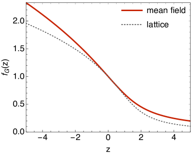
Figure 1: (a) A comparison of the mean field magnetic EOS to numerical results from lattice methods taken from Engels and Karsch (2014, 2012). (b) The sigma and pion screening masses (inverse correlation lengths), $m_{\sigma}$ and $m$, compared to results from lattice methods. The lattice curves were obtained by digitizing the numerical data from Fig. 8 and Fig. 9 of Engels et al. (2003), which was subsequently fit with a parametrized form.

II.2 Static correlation functions in mean field

Given the mean value $\bar{\sigma}$, we can evaluate the action (3) to quadratic order

$${S}_{E}=\beta\int d^{3}x\,\left[p_{\sigma}(T)+\frac{1}{2}\chi_{0}\mu^{2}-\frac{1}{2}\left(\partial_{i}\delta\sigma\,\partial^{i}\delta\sigma+m_{\sigma}^{2}\delta\sigma^{2}\right)-\frac{1}{2}\left(\partial_{i}\vec{\pi}\cdot\partial^{i}\vec{\pi}+m^{2}\vec{\pi}^{2}\right)\right],$$ (15)

where

$$p_{\sigma}(T)=p_{0}(T)-\left(\frac{1}{2}m_{0}^{2}(T)\bar{\sigma}^{2}(T)+\frac{\lambda}{4}\bar{\sigma}(T)^{4}-H\bar{\sigma}(T)\right)\,.$$ (16)

The sigma and pion screening masses are

$$m_{\sigma}^{2} \equiv m_{c}^{2}\left(z+3f_{G}^{2}(z)\right)\,,$$ (17a)

$$m^{2} \equiv\frac{H}{\bar{\sigma}(T)}=\frac{m_{c}^{2}}{f_{G}(z)}\,.$$ (17b)

As in the previous section, the screening masses (or inverse correlation lengths) are also defined outside of mean field theory. These are expected to scale as

$$m_{\sigma}= {\mathfrak{m}}_{L}\,h^{\nu_{c}}\,g_{L}(z)\,,$$ (18)

$$m= {\mathfrak{m}}_{T}\,h^{\nu_{c}}\,g_{T}(z)\,,$$ (19)

where ${\mathfrak{m}}_{L}$ and ${\mathfrak{m}}_{T}$ are non-universal constants, and $g_{L}(z)$ and $g_{T}(z)$ are universal scaling functions. As before, $g_{L}$ and $g_{T}$ are normalized to unity for $z=0$. The ratio between $m_{\sigma}$ and $m$ is also universal, and can be parameterized by $m_{\sigma}/m$ on the critical line, i.e. $m_{\sigma c}^{2}/m_{c}^{2}$. This universal ratio is compared to the mean field prediction of three in Table 1. $m(z)$ and $m_{\sigma}(z)$ are extracted from the numerical work of Ref. Engels et al. (2003) and compared to mean field theory in Fig. 1(b).

The quadratic action predicts the equal time correlation functions

$$\frac{1}{V}\left\langle\delta\sigma({\bm{k}})\delta\sigma(-{\bm{k}})\right\rangle =\frac{T}{k^{2}+m_{\sigma}^{2}}\,,$$ (20a)

$$\frac{1}{V}\left\langle\varphi_{s}({\bm{k}})\varphi_{s^{\prime}}(-{\bm{k}})\right\rangle =\frac{T}{\bar{\sigma}^{2}(k^{2}+m^{2})}\delta_{ss^{\prime}}\,.$$ (20b)

Finally, we can use the general theory of thermodynamics fluctuations to recognize that

$$\frac{1}{V}\left\langle n_{ab}({\bm{k}})n_{cd}(-{\bm{k}})\right\rangle =T\chi_{0}\,(\delta_{ac}\delta_{bd}-\delta_{ad}\delta_{bc})\,.$$ (22)

Well below $T_{c}$, the pion mass is small and soft pions are long lived quasi-particles Son (2000); Son and Stephanov (2002a, b). From this context we introduce a number of definitions following Son and Stephanov Son and Stephanov (2002b). The phase of the condensate is

$$\varphi_{s}\equiv\frac{\pi_{s}}{\bar{\sigma}}\,,$$ (23)

while the associated the pion velocity squared is

$$v^{2}(T)\equiv\frac{\bar{\sigma}^{2}(T)}{\chi_{0}}.$$ (24)

The pole mass is defined as $m_{p}^{2}\equiv v^{2}m^{2}$, and the soft pion dispersion curve takes the form

$$\omega^{2}_{q}=v^{2}q^{2}+m_{p}^{2},$$ (25)

which is parameterized by two Euclidean quantities $v^{2}(T)$ and $m^{2}(T)$.

In the next section we will develop the hydrodynamic theory for the $O(4)$ model. The real time correlation functions constructed from this theory will reproduce (20) and (22) after integrating over frequency.

III Hydrodynamics

Having discussed the thermodynamics, we are ready to derive the corresponding hydrodynamic theory. The resulting equations of motion are equivalent to those derived previously by Rajagopal and Wilczek using Poisson bracket methods Rajagopal and Wilczek (1993). Well below $T_{c}$, the equations of motion resemble a non-abelian superfluid theory and also have been analyzed Son (2000); Son and Stephanov (2002b); Jain (2017); Grossi et al. (2020). The methodology here follows closely our previous work Grossi et al. (2020).

III.1 Ideal hydrodynamics and the Josephson constraint

To derive the ideal hydrodynamic expressions we follow an expedient procedure procedure outlined in Jensen et al. (2012) and take as hydrodynamic action

$${S}[g_{\mu\nu},A_{\mu},H]=\int d^{4}x\sqrt{-g}\,p_{\Sigma}(T,\mu,(\partial_{\perp}\phi)^{2},\phi^{2},H\cdot\phi)\,,$$ (26)

where the redefined pressure takes the same form as its Euclidean counterpart

$$p_{\Sigma}(T,\mu,(\partial_{\perp}\phi)^{2},\phi^{2},H\cdot\phi)\equiv p(T)+\frac{1}{4}\chi_{0}\,\mu\cdot\mu-\frac{1}{2}\Delta^{\mu\nu}D_{\mu}\phi\cdot D_{\nu}\phi-V({\Phi})+H\cdot\phi\,,$$ (27)

but we have replaced the integration over thermal circle with an integration over time

$$\beta=\int_{0}^{\beta}d\tau\rightarrow\int dt\,.$$ (28)

We also have added external gauge and gravitational fields, $(A_{\mu})_{ab}$ and $g_{\mu\nu}$, for the purpose of deriving the stress tensor and currents, and ultimately these sources will be set to zero. In these expressions $T\equiv(-\beta^{\mu}g_{\mu\nu}\beta^{\mu})^{-1/2}$, and then we define $u^{\mu}\equiv T\beta^{\mu}$, and $\Delta^{\mu\nu}\equiv g^{\mu\nu}+u^{\mu}u^{\nu}$. The chemical potential can be written

$$\mu_{ab}=\left(u^{\rho}\tilde{\mu}_{\rho}+u^{\rho}A_{\rho}\right)_{ab}\,,$$ (29)

where $(\tilde{\mu}_{\rho})_{ab}$ is the contact chemical potential and is independent of $A_{\rho}$. The covariant derivative is

$$(D_{\mu}\phi)_{a}=\partial_{\mu}\phi_{a}-\tfrac{i}{2}(A_{\mu}\cdot\mathcal{J})_{ab}\phi_{b}\,,$$ (30)

where $\mathcal{J}_{cd}$ are the generators $O(4)$ rotation group

$$(i\mathcal{J}_{cd})_{ab}=\delta_{ca}\delta_{db}-\delta_{cb}\delta_{da}\,.$$ (31)

Setting the external fields to zero for simplicity, the differential of pressure at fixed $H$ follows from the form of $p_{\Sigma}$

$$dp_{\Sigma}=s_{\Sigma}\,dT+\frac{1}{2}n_{ab}\,d\mu_{ab}-\frac{1}{2}d(\partial_{\perp}^{\mu}\phi)^{2}+\left(-\frac{\partial V}{\partial\phi_{a}}+H_{a}\right)d\phi_{a}\,,$$ (32)

which defines the entropy density, $s_{\Sigma}\equiv\partial p_{\Sigma}/\partial T$, and the number densities, $n_{ab}\equiv 2\,\partial p_{\Sigma}/\partial\mu_{ab}$, respectively. Here and below $d\equiv u^{\mu}\partial_{\mu}$ and $\partial_{\perp}^{\mu}=\Delta^{\mu\nu}\partial_{\nu}$.

Varying the action with respect to the metric yields the conserved stress tensor $\partial_{\mu}T^{\mu\nu}=0$. Recognizing that both the temperature and the chemical potential depend implicitly on the metric after they are written in terms of $\beta^{\mu}$, the variation of the action gives

$$T^{\mu\nu}=\left.\frac{2}{\sqrt{-g}}\frac{\delta{S}}{\delta g_{\mu\nu}}\right|_{g=A=0}=(\varepsilon_{\Sigma}+p_{\Sigma})\,u^{\mu}u^{\nu}+p_{\Sigma}g^{\mu\nu}+\partial^{\mu}\phi\cdot\partial^{\nu}\phi-u^{\mu}u^{\nu}(u^{\sigma}\partial_{\sigma}\phi)\cdot(u^{\rho}\partial_{\rho}\phi),$$ (33)

where in this expression the energy density has been defined through the Gibbs-Duhem relation

$$\varepsilon_{\Sigma}=-p_{\Sigma}+Ts_{\Sigma}+\tfrac{1}{2}\mu_{ab}\cdot n_{ab}\,.$$ (34)

We can find the partial current conservation equation by requiring that the action in (26) be invariant under gauge transformations. We will limit the discussion to weak fields and switch off the gravitational field for this purpose. Under an infinitesimal $O(4)$ rotation with parameters $\omega_{cd}(x)$, the gauge fields and magnetic field transform as

$$A_{\mu,cd}\rightarrow A_{\mu,cd}+\partial_{\mu}\omega_{cd}\,,$$ (35a)

$$\delta H_{a}\rightarrow H_{a}+\tfrac{i}{2}(\omega\cdot{\mathcal{J}})_{ab}H_{b}\,.$$ (35b)

Then, requiring invariance of the action under the rotation,

$$\delta{S}= \int d^{4}x\,\frac{\delta{S}}{\delta A_{\mu,ab}}\,\delta A_{\mu,ab}+\frac{\delta{S}}{\delta H_{a}}\delta H_{a}=0,$$ (36)

and inserting the transformation rules (35), we find partial current conservation

$$\partial_{\mu}J^{\mu}_{cd}=\phi_{c}H_{d}-\phi_{d}H_{c}\,.$$ (37)

Here the currents are given by

$$J^{\mu}_{ab}\equiv 2\frac{\delta{S}}{\delta A_{\mu,ab}}=\chi_{0}\mu_{ab}u^{\mu}+(J^{\mu}_{\perp})_{ab}\,,$$ (38)

where the first term is the normal component and the second term is the superfluid component, given by

$$(J_{\perp})_{ab}^{\mu}=\Delta^{\mu\nu}(\partial_{\nu}\phi_{a}\phi_{b}-\partial_{\nu}\phi_{b}\phi_{a}).$$ (39)

To complete the equations of motion of ideal hydrodynamics, we need to specify a relationship between the phase of the condensate and the chemical potential known as the Josephson constraint. The Josephson constraint is the requirement that the field $\phi_{a}$ is stationary under the evolution generated by the grand potential, $\Omega=H-\frac{1}{2}\mu_{bc}N_{bc}$, i.e. the stability of the thermal state. This reasoning leads to a requirement on the classical Poisson bracket between $\phi$ and $\Omega$

$$\{\phi_{a},\Omega\}=\{\phi_{a},-u^{\mu}P_{\mu}-{\textstyle\frac{1}{2}}\mu_{bc}N_{bc}\}=0\,.$$ (40)

Recalling that $P_{\mu}$ and $N_{ab}$ generate translations and rotations respectively (which determines their Poisson brackets with $\phi$), we find

$$u^{\mu}\partial_{\mu}\phi_{a}+{\textstyle\frac{1}{2}}(\mu_{ab}\phi_{b}-\phi_{b}\mu_{ba})=0\,.$$ (41)

Alternatively, but ultimately equivalently, the Josephson constraint can be derived by requiring entropy conservation at ideal order Jain (2017)

$$\partial_{\mu}(s_{\Sigma}u^{\mu})=0.$$ (42)

Appendix A uses the conservation laws together with the Gibbs-Duhem relation (34) and the pressure differential (32) to show that entropy is only conserved if the Josephson constraint is satisfied. When viscous corrections are included at subsequent orders in the gradient expansion, the Josephson constraint will need to be modified.

Finally, it is useful to express the Josephson constraint in terms of the amplitude, $\Phi$, and $SU(2)$ phase, $U$. Writing the chiral condensate as

$$\Sigma=\phi_{a}\tau_{a}=\Phi U\,,$$ (43)

the Josephson constraint can be written

$$u^{\mu}\partial_{\mu}\Phi =0\,,$$ (44a)

$$iu^{\mu}\partial_{\mu}UU^{-1} =\mu_{L}-U\mu_{R}U^{\dagger}\,,$$ (44b)

where $\mu_{L}=\tfrac{1}{2}\mu_{ab}\tau_{ab}$ and $\mu_{R}=\tfrac{1}{2}\mu_{ab}\bar{\tau}_{ab}$ are the left and right chemical potentials. The last relation between the phase and the chemical potentials is familiar from non-abelian superfluids Son (2000); Grossi et al. (2020)

III.2 Viscous corrections

So far we have considered only the ideal equations of motion. In the dissipative case the energy-momentum tensor, the charge current, and the Josephson constraint will acquire new terms that correspond to dissipation into the system. The energy-momentum tensor and the conserved currents are modified due to dissipative effects in the usual way:

$$T^{\mu\nu} =T^{\mu\nu}_{\text{ideal}}+\Pi^{\mu\nu},$$ (45)

$$J_{ab}^{\mu} =J_{ab,\text{ideal}}^{\mu}+q^{\mu}_{ab}.$$ (46)

We will work in the Landau frame, where the dissipative contributions to the stress tensor and the diffusion current are taken to be orthogonal to the four velocity $u^{\mu}$, i.e.

$$\Pi^{\mu\nu}u_{\mu}=0,\quad q^{\mu}_{ab}u_{\mu}=0.$$ (47)

The stress tensor can be further decomposed into a symmetric-traceless and transverse part, $\pi^{\mu\nu}$, and a trace part, $\Pi$,

$$\Pi^{\mu\nu}=\pi^{\mu\nu}+\Pi\Delta^{\mu\nu}.$$ (48)

In addition to the dissipative corrections to the energy-momentum tensor and the current, the evolution equation of the chiral condensate, $\phi_{a}$, gets modified by dissipative effects. Therefore it is useful to define

$$u^{\mu}\partial_{\mu}\phi_{a}+\mu_{ab}\phi_{b}=\Xi_{a},$$ (49)

where $\Xi_{a}$ is a Lorentz scalar that encodes the dissipative contribution to the scalar field equation of motion.

Using the conservation of the energy-momentum tensor and the partial conservation of the charge, the Gibbs-Duhem relation in (34), and the pressure differential in (32) we can derive the entropy production as

$$\partial_{\mu}(s_{\Sigma}u^{\mu}-\frac{\mu_{ab}}{2T}q^{\mu}_{ab})=\frac{\Xi_{a}}{T}\Theta_{a}-\partial_{\mu}\left(\frac{u_{\nu}}{T}\right)\Pi^{\mu\nu}-\partial_{\mu}\left(\frac{\mu_{ab}}{2T}\right)q^{\mu}_{ab}.$$ (50)

where we have defined the scalar quantity

$$\Theta_{a}=\partial^{2}_{\perp}\phi_{a}-\frac{\partial V}{\partial\phi_{a}}+H_{a},$$ (51)

with $\partial_{\perp}^{2}\phi_{a}\equiv\partial_{\mu}\partial^{\mu}_{\perp}\phi_{a}$.

Up to now we have not specified an expansion scheme; the equations are just a consequence of the definition of entropy, the conservation of energy and momentum, and the partial conservation charge. The positivity of entropy production in the tensor sector can be enforced with

$$\pi^{\mu\nu}=-\eta_{\Sigma}\sigma^{\mu\nu},\quad\text{with}\quad\eta_{\Sigma}\geq 0,$$ (52)

where $\eta_{\Sigma}$ is the shear viscosity of the $O(4)$ theory. In the vector sector we have

$$q_{ab}^{\mu}=-T\sigma_{\Sigma}\partial^{\mu}\left(\frac{\mu_{ab}}{T}\right),\quad\text{with}\quad\sigma_{\Sigma}\geq 0\,,$$ (53)

where $\sigma_{\Sigma}$ is the $O(4)$ conductivity.

The scalar sector requires a bit more care as there are two Lorentz scalars, $\Xi_{a}\Theta_{a}$ and $\Pi\,\partial_{\mu}u^{\mu}$. Generally we have as the constitutive relations for $\Pi$ and $\Xi_{a}$

$$\Pi =-\zeta_{\Sigma}\,\partial_{\mu}u^{\mu}-\zeta^{(1)}_{\Sigma}\,\phi_{a}\Theta_{a},$$ (54)

$$\Xi_{a} =\zeta^{(1)}_{\Sigma}\,\phi_{a}\partial_{\mu}u^{\mu}+\Gamma\,\Theta_{a},$$ (55)

where $\zeta_{\Sigma}$ is the bulk viscosity, $\zeta^{(1)}_{\Sigma}$ and $\Gamma$ are the transport coefficients regulating the dissipative effects of the scalar field dynamics. The positivity of the associated quadratic form is enforced if

$$\zeta_{\Sigma}\geq 0,\quad\Gamma\geq 0,\quad\text{ and }\quad\zeta_{\Sigma}\,\Gamma-(\zeta^{(1)}_{\Sigma})^{2}\,\phi^{2}\geq 0.$$ (56)

Having specified the dissipative fluxes, it is possible to write down the energy-momentum tensor, the current, and the scalar field equation, including the first gradient corrections. The scalar field obeys a relaxation-type equation where the ideal part is the Josephson constraint

$$u^{\mu}\partial_{\mu}\phi_{a}+\mu_{ab}\phi_{a}=\Gamma\left[\partial^{2}_{\perp}\phi_{a}-\frac{\partial V}{\partial\phi_{a}}+H_{a}\right]+\zeta^{(1)}_{\Sigma}\phi_{a}\,\partial_{\mu}u^{\mu}.$$ (57)

The energy momentum tensor now includes dissipative contributions due to chiral condensate

$$\Pi^{\mu\nu}=-\eta_{\Sigma}\sigma^{\mu\nu}-\Delta^{\mu\nu}\left[\zeta_{\Sigma}\partial_{\mu}u^{\mu}-\zeta^{(1)}_{\Sigma}\phi_{\alpha}\left(\partial^{2}_{\perp}\phi_{a}-\frac{\partial V}{\partial\phi_{a}}+H_{a}\right)\right].$$ (58)

Finally the current has the form

$$(J^{\mu})_{ab}=n_{ab}u^{\mu}+(J^{\mu}_{\perp})_{ab}-T\sigma_{\Sigma}\,\Delta^{\mu\nu}\partial_{\nu}\left(\frac{\mu_{ab}}{T}\right)\,,$$ (59)

and is partially conserved as in (37). The coefficient $\zeta^{(1)}_{\Sigma}$ is an independent transport coefficient that couple the expansion rate $\partial_{\mu}u^{\mu}$ to the Josephson constraint and vice versa. Near the phase transition $\phi_{\alpha}$ is approximately zero, which means this term is subdominant and can be neglected.

Let us compare these equations to a number of results in the literature. The equations are equivalent to those of Rajagopal and Wilczek written down almost thirty years ago Rajagopal and Wilczek (1993); our notation for $\sigma_{\Sigma}$ and $\Gamma$ follows theirs. The current reformulation is covariant and includes the coupling to the background flow. In the low temperature limit the equations match those of our previous paper Grossi et al. (2020) (which includes a discussion of earlier work Son (2000); Son and Stephanov (2002b)), provided one identifies some of the coefficients.

III.3 Linear response

Knowing the equations of motion we can determine the hydrodynamic predictions for the retarded Green functions of the system. In the axial channel we can consider the coupled equations of motion for $\varphi_{s}$ and the axial chemical potential $\mu_{0s}$, when $\phi_{a}$ is linearized around equilibrium

$$\phi_{a}= (\bar{\sigma},-\bar{\sigma}\varphi_{s})\,.$$ (60)

To find the response function for $(\omega_{k}\varphi_{s},\mu_{0s})$, we introduce a pseudoscalar source $H_{a}=(H,\delta H_{s}(x))$ and a gauge field $(A_{0}(x))_{0s}$ which are conjugate to $-\sigma\varphi_{s}$ and $\chi_{0}\mu_{0s}$ respectively. Due to the $O(4)$ symmetry, the external gauge field can appear in the time derivative of $\varphi_{s}$ and spatial gradient of the chemical potential

$$\partial_{t}\phi_{s} \to D_{t}\phi_{s}=\partial_{t}\phi_{s}-(A_{0})_{s0}\bar{\sigma},$$ (61a)

$$\partial_{i}\mu_{0s} \rightarrow\partial_{i}\mu_{0s}-(E_{i})_{0s},$$ (61b)

where $(E_{i})_{0s}=(\partial_{i}A_{0})_{0s}$. Applying these transformations and Fourier transforming leads us to the linearized equations in matrix form

$$\begin{pmatrix}-i\omega+\Gamma(k^{2}+m^{2})&\omega_{k}\\ -\omega_{k}&-i\omega+Dk^{2}\\ \end{pmatrix}\begin{pmatrix}\omega_{k}\varphi_{s}\\ \mu_{0s}\end{pmatrix}=\frac{1}{\chi_{0}}\begin{pmatrix}\Gamma(k^{2}+m^{2})&\omega_{k}\\ -\omega_{k}&Dk^{2}\\ \end{pmatrix}\begin{pmatrix}-\bar{\sigma}\delta H_{s}/\omega_{k}\\ \chi_{0}(A_{0})_{0s}\end{pmatrix},$$ (62)

where we have defined the diffusion coefficient $D=\sigma_{\Sigma}/\chi_{0}$ of the $O(4)$ symmetric theory. The linearized equations can be solved to find the retarded propagator

$$\begin{pmatrix}\omega_{k}\varphi_{s}\\ \mu_{0s}\end{pmatrix}=\frac{1}{\chi_{0}}\frac{1}{(-\omega^{2}+\omega_{k}^{2}+g_{1}g_{2})-i\omega\Gamma_{k}}\\ \times\begin{pmatrix}g_{1}(g_{2}-i\omega)+\omega_{k}^{2}&-i\omega\omega_{k}\\ i\omega\omega_{k}&g_{2}(g_{1}-i\omega)+\omega_{k}^{2}\\ \end{pmatrix}\begin{pmatrix}-\bar{\sigma}\delta H_{s}/\omega_{k}\\ \chi_{0}\,(A_{0})_{0s}\end{pmatrix}\,,$$ (63)

where, for compactness, we define the following shorthand for the dissipative rates:

$$g_{1} \equiv\Gamma(k^{2}+m^{2})\,,$$ (64a)

$$g_{2} \equiv Dk^{2}\,,$$ (64b)

$$\Gamma_{k} \equiv\Gamma(k^{2}+m^{2})+Dk^{2}=g_{1}+g_{2}\,.$$ (64c)

$\Gamma_{k}$ determines the damping rate of soft pions in the broken phase Son and Stephanov (2002b).

To compute the hydrodynamic loops in the next section, it will be necessary to use the symmetrized propagator

$$[G_{\rm sym}(\omega)]=\frac{T}{\omega}\frac{[G_{R}(\omega)]-[G_{A}(\omega)]}{i}\equiv\frac{T}{\omega}[\rho(\omega,k)],$$ (65)

where the advanced propagator is

$$[G_{A}(\omega)]=[G_{R}(\omega)]^{\dagger},$$ (66)

and $\rho$ notates the spectral density. Thus, the symmetrized propagator is

$$[G_{\rm sym}(\omega)]=\frac{2T}{\chi_{0}}\frac{1}{(-\omega^{2}+\omega_{k}^{2}+g_{1}g_{2})^{2}+(\omega\Gamma_{k})^{2}}\begin{pmatrix}g_{1}(\omega^{2}+g_{2}^{2})+g_{2}\omega_{k}^{2}&-i\omega_{k}\omega\Gamma_{k}\\ i\omega_{k}\omega\Gamma_{k}&g_{2}(\omega^{2}+g_{1}^{2})+g_{1}\omega_{k}^{2}\end{pmatrix}.$$ (67)

In Fig. 2 we exhibit the spectral density for several values of the scaling variable $z$ and a specific choice of parameters discussed below. It is instructive to analyze the spectral density in the pion-axial charge channel in two different limits, the broken phase, $z\to-\infty$, and the symmetric phase, $z\to\infty$.

In the broken phase $z\to-\infty$, the field expectation value $\bar{\sigma}$ is large and $\omega_{k}\gg g_{1,2}$. In this limit the spectral density approaches a Breit-Wigner form with the peaks given by the quasi-particle dispersion relation $\omega=\pm\omega_{k}$ and a width given by $\Gamma_{k}$ Son and Stephanov (2002b). Then the denominator in the spectral density can be approximated as

$$\frac{\Gamma_{k}}{(-\omega^{2}+\omega_{k}^{2}+g_{1}g_{2})^{2}+(\omega\Gamma_{k})^{2}}\sim\frac{1}{4\omega_{k}^{2}}\left[\rho(\omega,\omega_{k})+\rho(\omega,-\omega_{k})\right],$$ (68)

where $\rho(\omega,\omega_{k})$ notates the Breit-Wigner form

$$\rho(\omega,\omega_{k})=\frac{\Gamma_{k}}{(-\omega+\omega_{k})^{2}+(\Gamma_{k}/2)^{2}}.$$ (69)

In this limit, we can simplify the expression of the spectral density, leading to

$$[\rho(\omega)]=\frac{\omega}{2\chi_{0}}\left[\rho(\omega,\omega_{k})+\rho(\omega,-\omega_{k})\right]\begin{pmatrix}1&-i\\ i&1\end{pmatrix}+\mathcal{O}\left(\frac{\Gamma_{k}}{\omega_{k}}\right).$$ (70)

Thus, there is a relation between the spectral density of pions and the axial charge

$$\rho_{AA}(\omega,k)=i\chi_{0}\omega_{k}\,\rho_{\varphi A}(\omega,k)=(\chi_{0}\omega_{k})^{2}\,\rho_{\varphi\varphi}\,,$$ (71)

which is a manifestation of the PCAC relations. These relations are the direct consequences of the Josephson equation, $-\partial_{t}\varphi=n_{A}/\chi_{0}$. Indeed, due to the ideal equation of motion for the field $\varphi_{s}$, we have

$$\rho_{AA}(\omega,k)=-\chi_{0}\,\rho_{\partial_{t}\varphi A}(\omega,k)=\chi_{0}^{2}\,\rho_{\partial_{t}\varphi\partial_{t}\varphi}(\omega,k)\,,$$ (72)

which highlights that the axial charge and the time derivative of the pion field are two interchangeable concepts.

As the temperature increases, the real and imaginary parts of the propagator become of the same order of magnitude $\omega_{k}\sim g_{1}g_{2}$, and the parameter that governs their relative importance can be taken as

$$u^{2}=\frac{\omega^{2}_{k}}{g_{1}g_{2}}\Big{|}_{k=m}=\frac{v^{2}}{\Gamma Dm^{2}}.$$ (73)

At the phase transition, $z=0$, where $m=m_{c}$ and $v=v_{c}$ it is natural to assume that the real and imaginary part are the same order of magnitude Son and Stephanov (2002b), and therefore here we will consider the case where

$$u^{2}_{c}=\frac{v_{c}^{2}}{\Gamma Dm_{c}^{2}}=1.$$ (74)

The propagator also depends on a another dimensionless parameter

$$r^{2}=\frac{\Gamma}{\Gamma+D},$$ (75)

which expresses the relative strengths of the axial diffusion and the order parameter relaxation. Calculations from chiral perturbation theory found the value $r^{2}=3/4$ Teaney et al. , and we will adopt this number as an estimate for this order one constant.

In the symmetric phase $z\to\infty$, the field expectation value is very small $\bar{\sigma}\sim 0$ and $v^{2}\sim 0$. Thus, the spectral density matrix becomes diagonal

$$[\rho(\omega)]_{z\to\infty}=\frac{2\omega}{\chi_{0}}\frac{1}{(\omega^{2}+g_{2}^{2})(\omega^{2}+g_{1}^{2})}\begin{pmatrix}g_{1}(\omega^{2}+g_{2}^{2})&0\\ 0&g_{2}(\omega^{2}+g_{1}^{2})\end{pmatrix}\,,$$ (76)

and the pion and axial charge are completely decoupled. The pion field simply relaxes to zero and the axial charge is purely diffusive. The spectral density of axial charge is therefore

$$\rho_{AA}(\omega,k)=\frac{2\omega\chi_{0}Dk^{2}}{(\omega^{2}+(Dk^{2})^{2})},$$ (77)

while in the pion channel we have

$$\bar{\sigma}^{2}\rho_{\varphi\varphi}(\omega,k)=\frac{2\omega\Gamma}{\omega^{2}+\Gamma^{2}(k^{2}+m^{2})^{2}},$$ (78)

which exhibits a simple relaxation pole with relaxation rate $\Gamma(k^{2}+m^{2})$. In the symmetric phase the axial charge and the pions are completely disentangled, and their dissipative dynamics is controlled by two distinct transport coefficients.

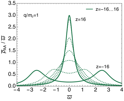
Figure 2: The spectral density $\rho_{AA}(\omega,q)$ for the axial charge density-density correlator with the scaling variable $z\equiv th^{-2/3}$ taking values $z=-16,-4,-1,0,1,4,16$. For large positive $z$ the distribution asymptotes to the simple diffusive pole, $\rho_{AA}/\omega\propto Dk^{2}/(\omega^{2}+(Dk^{2})^{2})$, reflecting the diffusion of quarks. For large negative $z$ the pair of peaks reflects the propagating pions. We have rescaled the axes, defining $\bar{\omega}\equiv\omega/\Gamma m_{c}^{2}$ and $\bar{\rho}_{AA}(\omega)=\rho_{AA}(\omega,q)/2\chi_{0}$, and chosen $q/m_{c}=1$ for illustration. For definiteness, we have set $D/\Gamma=1/3$, and $v^{2}_{c}/\Gamma Dm^{2}_{c}=1$, and the motivation for these constants is given in the text surrounding eq. (73).

Moving to the $\sigma$ contribution, we see that the linearized equation of motion is

$$\partial_{t}\delta\sigma=\Gamma(\nabla^{2}-m_{\sigma}^{2})\,\delta\sigma+\Gamma\delta H\,,$$ (79)

where we have added an external source to the scalar field, $H\rightarrow H+\delta H$. Solving in Fourier space, we see that the retarded Green’s function is

$$G_{R}^{\sigma\sigma}(\omega,k)=\frac{\Gamma}{-i\omega+\Gamma(k^{2}+m_{\sigma}^{2})}\,,$$ (80)

and the symmetrized propagator is

$$G_{\rm sym}^{\sigma\sigma}=\frac{2T\Gamma}{\omega^{2}+\Gamma^{2}(k^{2}+m_{\sigma}^{2})^{2}}.$$ (81)

In the symmetric case ($z\to\infty$) the propagator of $\delta\sigma$ and $\varphi$ become degenerate and $O(4)$ symmetric

$$\rho_{\sigma\sigma}(\omega,k)=\bar{\sigma}^{2}\rho_{\varphi\varphi}(\omega,k),$$ (82)

with $m^{2}=m_{\sigma}^{2}$.

IV Transport coefficients

In this section we will use the response functions calculated in the previous section to determine the current-current and stress-stress correlation functions. This will determine the critical behavior of the transport coefficients, which is analyzed and estimated in Sect. IV.2.

IV.1 Hydrodynamic loops

In the critical hydrodynamic theory we outlined in Sect. III, we have integrated out modes of order $k\sim T$. These modes are incorporated into the transport coefficients such as $\eta_{\Sigma}$ and its associated noise, $\xi_{\eta_{\Sigma}}^{\mu\nu}$. Modes of order $k\sim m_{\sigma}$ are explicitly propagated in the theory, and the critical hydrodynamic theory is defined with a cutoff $\Lambda_{T}$

$$k\sim m_{\sigma}\ll\Lambda_{T}\ll T.$$ (83)

In normal hydrodynamics, modes with $k\sim m_{\sigma}$ are integrated out and incorporated into the transport coefficients of the normal theory, such as $\eta$ and its noise. The only modes which are explicitly propagated are the conserved charges, and the theory is defined with a cutoff $\Lambda_{\sigma}$

$$k\ll\Lambda_{\sigma}\ll m_{\sigma}\,.$$ (84)

The two transport coefficients $\eta_{\Sigma}$ and $\eta$ may be related by integrating out modes between $k\in[\Lambda_{\sigma},\Lambda_{T}]$.

The $xy$ components of the stress tensor in the critical hydrodynamic theory is

$$T^{xy}= \partial^{x}\delta\sigma\,\partial^{y}\delta\sigma+\bar{\sigma}^{2}\partial^{x}\varphi_{s}\partial^{y}\varphi_{s}+\xi^{xy}_{\eta_{\Sigma}},$$ (85)

where the noise satisfies

$$\left\langle\xi_{\eta_{\Sigma}}^{xy}(x_{1})\xi_{\eta_{\Sigma}}^{xy}(x_{2})\right\rangle=2T\eta_{\Sigma}\delta^{4}(x_{1}-x_{2})\,.$$ (86)

It is understood that the noise in the critical hydrodynamic theory is only local on scales with $k\ll\Lambda_{T}$, i.e. the $\delta$-function in (86) should be cutoff at the scale $\Lambda_{T}$ and associated with a scale-dependent parameter, $\eta_{\Sigma}(\Lambda_{T})$. The stress tensor in the normal hydrodynamic theory is simply the noise (in the absence of external flow)

$$T^{xy}_{\rm hydro}=\xi^{xy}_{\eta}(x)\,,$$ (87)

and satisfies

$$\left\langle\xi_{\eta}^{xy}(x_{1})\xi_{\eta}^{xy}(x_{2})\right\rangle=2T\eta\delta^{4}(x_{1}-x_{2})\,.$$ (88)

Matching the two effective theories yields Kubo formulas, which require that the integrated variances of the fluctuations are equal in the two theories Forster (1995):

$$2T\eta=\int d^{4}x\left\langle T^{xy}_{\rm hydro}(t,\bm{x})T^{xy}_{\rm hydro}(0,{\bm{0}})\right\rangle=\int d^{4}x\left\langle T^{xy}(t,\bm{x})T^{xy}(0,{\bm{0}})\right\rangle\,.$$ (89)

Incorporating the fluctuations of $\sigma$ and $\varphi$ at one loop, this evaluates to

$$2T\eta =2T\eta_{\Sigma}(\Lambda_{T})+2\int^{\Lambda_{T}}\frac{d^{3}k}{(2\pi)^{3}}\frac{d\omega}{2\pi}\left[(k^{x}k^{y}G_{\rm sym}^{\sigma\sigma})^{2}+d_{A}\frac{\bar{\sigma}^{4}}{\omega_{k}^{4}}(k^{x}k^{y}G_{\rm sym}^{\varphi\varphi})^{2}\right],$$ (90)

where we have anticipated a divergence which is regulated at the scale $\Lambda_{T}$, as is appropriate for the critical hydrodynamic theory.

The other transport coefficients of interest here are expressed similarly as

$$2T\sigma_{I}= \int d^{4}x\frac{1}{d_{A}}\left\langle{\textstyle\frac{1}{2}}\{J_{V,s}^{x}(t,{\bm{x}}),J_{V,s}^{x}(0,{\bm{0}})\}\right\rangle,$$ (91)

$$2T\zeta= \int d^{4}x\left\langle{\textstyle\frac{1}{2}}\left\{{\mathcal{O}}_{\rm bulk}(t,{\bm{x}}),{\mathcal{O}}_{\rm bulk}(0,{\bm{0}})\right\}\right\rangle.$$ (92)

where ${\mathcal{O}}_{\rm bulk}=\tfrac{1}{3}T^{i}_{i}+c_{s}^{2}T^{0}_{0}$. The bulk viscosity is significantly more complicated, and quite susceptible to physics which goes beyond the mean field approach adopted here. Therefore we will evaluate the bulk viscosity only in the high temperature symmetric regime. The relevant operators appearing in the conductivity computation and the bulk viscosity are

$$J^{x}_{V,s} =\bar{\sigma}^{2}\epsilon_{ss^{\prime}s^{\prime\prime}}\varphi_{s^{\prime}}\partial^{x}\varphi_{s^{\prime\prime}},$$ (93)

$$O_{\rm bulk,\infty} =\frac{1}{2}c_{s}^{2}{\mathfrak{m}}^{2}(\delta\sigma^{2}+\pi^{2}).$$ (94)

Here and below we use the $\infty$ subscript to indicate that we have made approximations of $O_{\rm bulk}$ appropriate only in the symmetric phase where $z$ is large. We have also recognized that near $T_{c}$ the terms stemming from $c_{s}^{2}T^{0}_{0}$ are parametrically large compared to $T^{i}_{i}$. Evaluating the relevant Feynman diagrams leads to

$$2T\sigma_{I} =2T\sigma_{\Sigma}+2T_{A}\bar{\sigma}^{4}\int\frac{d^{3}k}{(2\pi)^{3}}\frac{d\omega}{2\pi}\frac{1}{\omega_{k}^{4}}(k^{x}G_{\rm sym}^{\varphi\varphi})^{2}\,,$$ (95)

$$2T\zeta_{\infty} \approx 2T\zeta_{\Sigma}+2\left(\tfrac{1}{2}c_{s}^{2}{\mathfrak{m}}^{2}\right)^{2}\int\frac{d^{3}k}{(2\pi)^{3}}\frac{d\omega}{2\pi}\left[(G_{\rm sym}^{\sigma\sigma})^{2}+d_{A}(G_{\rm sym}^{\pi\pi})^{2}\right].$$ (96)

The propagators in these expressions can be read from (67) and (81). The $\sigma$ and $\pi$ propagators at large $z$ which are used in (96) are the same and are given in (81). To make the results of the above integrations more explicit we recall the dimensionless variables of Sect. III.3

$$r^{2}=\frac{\Gamma}{\Gamma+D},\quad\text{and}\quad u^{2}=\frac{v^{2}}{\Gamma Dm^{2}},$$

and introduce the symmetric, dimensionless function $f_{n}(r,u)=f_{n}(u,r)$, defined by

$$f_{n}(r,u) =\frac{16}{15\pi}\int_{0}^{\infty}\frac{dk}{m}\frac{k^{2n}}{(k^{2}+m^{2})^{3}}\frac{m^{8-2n}k^{2}}{(k^{2}+r^{2}m^{2})(k^{2}+u^{2}m^{2})}.$$ (97)

For the transport coefficients in question, we will need only the following explicit expressions

$$f_{3}(r,u) =\frac{1}{15\left(r^{2}-u^{2}\right)}\left[\frac{r^{2}\left(8r^{2}+9r+3\right)}{(r+1)^{3}}-\frac{u^{2}\left(8u^{2}+9u+3\right)}{(u+1)^{3}}\right],$$ (98)

$$f_{2}(u,r) =\frac{1}{15\left(r^{2}-u^{2}\right)}\left[\frac{r^{2}(3r+1)}{(r+1)^{3}}-\frac{u^{2}(3u+1)}{(u+1)^{3}}\right].$$ (99)

More details can be found in Appendix B. Then the conductivity, shear viscosity, and asymptotic bulk viscosity are given by

$$\sigma_{I}(z) =\sigma_{\Sigma}+\frac{TT_{A}}{32\pi m\Gamma}\left(1-5u^{2}(1-r^{2})f_{2}(r,u)\right)\,,$$ (100a)

$$\eta(z) =\eta_{\Sigma}-\frac{T}{32\pi\Gamma}(m_{\sigma}+md_{A}+md_{A}u^{2}(1-r^{2})f_{3}(r,u)),$$ (100b)

$$\zeta_{\infty}(z) =\zeta_{\Sigma}+\frac{T}{8\pi\Gamma m_{\sigma}^{3}}\left(\tfrac{1}{2}c_{s}^{2}{\mathfrak{m}}^{2}\right)^{2}.$$ (100c)

In these expressions the shear viscosity has been renormalized

$$\eta_{\Sigma} =\eta_{\Sigma}(\Lambda)+\delta_{aa}\,\frac{T\Lambda}{30\pi^{2}\Gamma},$$ (101a)

and the parameters $m(z)$, $m_{\sigma}(z)$, and $u^{2}(z)$, depend on the scaling variable $z$.

IV.2 Discussion

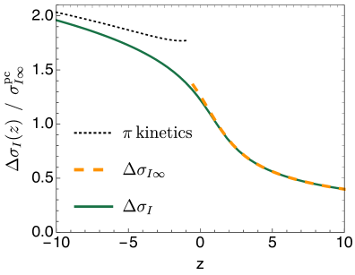
Figure 3: The critical contribution to the hydrodynamic transport coefficients, $\Delta\eta$and $\Delta\sigma_{I}$, as a function of the scaling variable $z=th^{-2/3}$. The asymptotic forms at large $z$ and small $z$, e.g. $\Delta\eta_{\infty}(z)$ and “pion kinetics” respectively, are discussed in text surrounding eq. (103). For the viscosity we have normalized the curve by a positive constant, $\eta^{\rm pc}_{\infty}\equiv|\Delta\eta_{\infty}(z_{\rm pc})|$, so that at the pseudo-critical point, $z_{\rm pc}=1.19$, the orange dashed asymptotic curve passes through minus one. We have defined $\sigma_{I\infty}^{\rm pc}$ with an analogous notation. The absolute magnitudes of these normalization constants are discussed in the text surrounding eq. (109). The curves depend weakly on two order one parameters, which we take to be $r^{2}$ and $u_{c}^{2}$ (see Fig. 2).

To gain an appreciation for the results of the previous section, in Fig. 3 we plot the critical contribution to the transport coefficients $\Delta\eta$ and $\Delta\sigma$ as a function of the scaling variable, $z$. The normalization of the curves and the asymptotics at large and small $z$ will be discussed shortly. We emphasize that Fig. 3 contains just the contribution from critical modes, e.g. the full shear viscosity takes the form

$$\eta(z)=\eta_{\Sigma}+\Delta\eta(z)\,,$$ (102)

where $\eta_{\Sigma}$ is a $z$ independent constant (the regular contribution to the shear viscosity).

At large positive $z$ the propagators for the $\sigma$ and $\pi$ fields become degenerate and take a simple form (see Sect. III.3). This greatly simplifies the computation of the hydrodynamic loop, leading to some simple forms for the critical transport corrections. Expanding our results in (100) for large $z$, or $u\rightarrow 0$, we find

$$\Delta\sigma_{\infty}(z) \equiv\frac{T}{16\pi m\Gamma},$$ (103a)

$$\Delta\eta_{\infty}(z) \equiv-\frac{Tm_{\sigma}}{8\pi\Gamma},$$ (103b)

$$\Delta\zeta_{\infty}(z) \equiv\frac{T}{8\pi\Gamma m_{\sigma}^{3}}\left(\tfrac{1}{2}c_{s}^{2}{\mathfrak{m}}^{2}\right)^{2}.$$ (103c)

These large $z$ asymptotics are presented as the (orange) dashed curves in Fig. 3. In these expressions $T$, ${\mathfrak{m}}^{2}$, $c_{s}$, and $\Gamma$ are constants near $T_{c}$, while the remaining functions, $m(z)$, $m_{\sigma}(z)$, are scaling functions which are determined by the equilibrium magnetic equation of state. Outside of the mean field approximation used here, $\Gamma$ is not a constant, but is expected to grow (fairly weakly) near the critical point as $\Gamma\sim m_{\sigma}^{d/2-2}\sim m_{\sigma}^{-1/2}$ Rajagopal and Wilczek (1993); Son and Stephanov (2002b). Treating $\Gamma$ and $D$ as constants is known in the literature as the van Hove approximation Hohenberg and Halperin (1977).

The asymptotic form of the transport coefficients sets the overall scale for our results. Thus in Fig. 3 we have divided each transport coefficient by a $z$-independent constant, the magnitude of the asymptotic result at the pseudo-critical point

$$\sigma_{\infty}^{\rm pc}\equiv \Delta\sigma_{\infty}(z_{\rm pc})\,,$$ (104a)

$$\eta_{\infty}^{\rm pc}\equiv |\Delta\eta_{\infty}(z_{\rm pc})|\,,$$ (104b)

$$\zeta_{\infty}^{\rm pc}\equiv \Delta\zeta_{\infty}(z_{\rm pc})|\,.$$ (104c)

Estimates for these scale coefficients in absolute units are given below. We also find that the simple asymptotic forms in (103) provide a useful order of magnitude estimate over the whole range in $z$, and in Fig. 4 we present the ratio between the full result and these forms. We expect that our asymptotic expression for the critical bulk viscosity in (103c) can provide a similarly good estimate over the whole range in $z$.

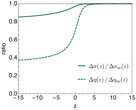
Figure 4: Ratio of the singular part of the transport coefficients to the asymptotic formulas (103) over the full range in $z$.

For large negative $z$, the $\sigma$ is significantly heavier than the pions, $m_{\sigma}\gg m$. We can integrate out the heavy sigma modes and pions with $p\sim m_{\sigma}$, leaving a local effective theory for soft pions with $p\sim m$. A hydrodynamic theory can be worked out for these soft pion modes coupled to the background stress Grossi et al. (2020). The (stochastic) hydrodynamic equations for the soft pions are equivalent to a Boltzmann equation in a “fluid metric”, which describes how the soft pions propagate in the background fluid Grossi et al. (2020). The collision terms of the kinetic equation are determined by the transport coefficients of the hydrodynamic theory. The computation of $\sigma$, $\eta$ and $\zeta$ at large negative $z$ could thus be done in two steps: first one would match the hydrodynamic equations at the critical point given in Sect. III to the soft-pion hydro-kinetic theory, and then one would use the soft-pion kinetic theory to determine the transport coefficients as a function of the temperature. For large negative $z$, the results predicted by the (matched) pion hydro-kinetic theory are shown by the black dotted curves in Fig. 3. The pion kinetic theory gives a reasonable description of the results of the full theory up to its boundary of applicability, $z\sim 0$. We will use the pion kinetic theory to estimate soft pion yields in Sect. V. Further details about the pion kinetic theory are given in Appendix C.

Now we will make several estimates for the absolute scales of the critical contribution to the transport coefficients, i.e. we wish to estimate $\eta_{\infty}^{\rm pc}$, $\zeta_{\infty}^{\rm pc}$, and $\sigma_{I\infty}^{\rm pc}$ defined in (104). These formulas have a number of physical quantities that need to be estimated, which we will do in the next paragraphs.

First, we consider the thermodynamic quantities, which are precisely determined by lattice measurements. To present each transport coefficient, we will first divide by the corresponding susceptibilities: $sT$ in the shear and bulk cases (the momentum susceptibility), and $T\chi_{Q}$ for the conductivity (the charge susceptibility). The pseudo-critical point is at $T_{\rm pc}\simeq 155\,{\rm MeV}$ Borsanyi et al. (2020). From lattice measurements of QCD thermodynamics at $T=155$ we have Borsanyi et al. (2010, 2014); Bazavov et al. (2012, 2014):

$$sT^{-3}=5.4\,,\qquad\chi_{Q}T^{-2}=0.4\,.$$ (105)

We will also need to estimate the screening masses, $m_{\sigma}$ and $m$, at these temperatures. At a temperature of $T_{\rm pc}=155$, we take from Table X of Ref. Bazavov et al. (2019)

$$m_{\sigma}(T_{\rm pc})=0.271\,{\rm GeV},\,\quad\text{and}\quad m(T_{\rm pc})=0.198\,{\rm GeV}\,.$$ (106)

The mean field predictions for $m_{\sigma}$ and $m$ are described in Sect. II; the one free mass parameter is adjusted so that the pion screening mass at the mean field pseudo-critical point at $z_{\rm pc}=1.19$ matches the lattice. The corresponding mean field $\sigma$ mass at $z_{\rm pc}=1.19$ is $m_{\sigma}=0.24\,{\rm GeV}$, which is slightly lower than the lattice results. To summarize, in our estimates below we take

$$m_{\sigma}/T=1.56,\quad\text{and}\quad m/T=1.28\,.$$ (107)

Finally, in order to evaluate the bulk viscosity we need to estimate ${\mathfrak{m}}^{2}$. In mean field theory we have

$$\frac{{\mathfrak{m}}^{2}}{T^{2}}=\frac{m_{\sigma}^{2}}{T^{2}}\left(-\frac{d\log\bar{\sigma}}{d\log T}\right)=\frac{m_{\sigma}^{2}}{T^{2}}\left(\frac{T_{c}}{T-T_{c}}\right)\left(-\frac{d\log f_{G}}{d\log z}\right)\simeq 7.0.$$ (108)

In making this estimate we have taken $T\simeq 155\,{\rm MeV}$ and $T_{c}\simeq 132\,{\rm MeV}$ Ding et al. (2019); Kaczmarek et al. (2020), and used the mean field equation of state. In absolute units ${\mathfrak{m}}\simeq 0.410\,{\rm GeV}$, which seems somewhat too low for a cutoff scale. Indeed $O(4)$ fits to lattice data suggest a somewhat higher value Kaczmarek et al. (2020).

The real time quantities in the transport coefficients are comparatively poorly determined. The two real time parameters are the order parameter relaxation coefficient $\Gamma$ and the diffusion coefficient $D$, which set the critical relaxation rates, $\Gamma m_{\sigma}^{2}\sim Dm_{\sigma}^{2}$. $D$ is regular near $T_{c}$ and determines the charge diffusion coefficient well above $T_{c}$. We will therefore adopt the strong coupling estimate, $D=1/2\pi T$ Son and Starinets (2007); Schäfer and Teaney (2009); Heinz and Snellings (2013), and we take $r^{2}=\Gamma/(\Gamma+D)=3/4$ and $v_{c}^{2}/\Gamma Dm_{c}^{2}=1$ as in Fig. 2 (see Sect. III.3 for further discussion).

Figure 5: The yields for soft pions due to a critical modification of the dispersion curve, relative to an expectation based on the vacuum dispersion curve (see eq. (121)). The results are shown for two different values of the cutoff $\Lambda$.

With these preliminaries we can estimate the scale factors for each transport coefficient.

$$\frac{\sigma_{I\infty}^{\rm pc}}{\chi_{Q}} =\frac{0.50}{2\pi T}\,\left[\left(\frac{1.5}{\pi T\Gamma}\right)\left(\frac{1.27}{m/T}\right)\left(\frac{0.4}{\chi T^{-2}}\right)\right],$$ (109a)

$$\frac{\eta_{\infty}^{\rm pc}}{sT} =\frac{0.3}{4\pi T}\,\left[\left(\frac{1.5}{\pi T\Gamma}\right)\left(\frac{5.4}{s/T^{3}}\right)\left(\frac{m_{\sigma}/T}{1.56}\right)\right],$$ (109b)

$$\frac{\zeta_{\infty}^{\rm pc}}{sT} =\frac{0.025}{4\pi T}\,\left[\left(\frac{1.5}{\pi T\Gamma}\right)\left(\frac{c_{s}^{2}}{0.2}\right)^{2}\left(\frac{{\mathfrak{m}}^{2}}{7.0\,T^{2}}\right)^{2}\left(\frac{5.4}{s/T^{3}}\right)\left(\frac{1.56}{m_{\sigma}/T}\right)^{3}\right].$$ (109c)

We have rescaled each transport coefficient by a value which is typical of strongly coupled plasmas Son and Starinets (2007); Schäfer and Teaney (2009). Thus, we see that the correction to the shear viscosity is small even in units of $1/4\pi$. The correction to the charge diffusion coefficient $D_{Q}=\sigma_{I}/\chi_{Q}$ is also modest, which is surprising given that this parameter diverges in the chiral limit. Evidently this parametrically large enhancement does not compensate for the overall kinematics of the loop integral. Similarly, the bulk viscosity is also parametrically enhanced by $m_{\sigma}^{-3}$, but in practice this also does not compensate for other kinematic factors. A similar observation about the bulk viscosity has been made previously in a somewhat different context Martinez et al. (2019).

V Outlook: chiral critical dynamics in heavy ion data?

The previous section estimated the influence of critical chiral modes on the transport coefficients of QCD. Given the rather large pion mass, these corrections are modest, and probably can not be observed in practice. However, it may be possible to observe the critical chiral fluctuations by directly measuring soft pions, rather than indirectly through their influence on the kinetics of the system. The approach in this section bears some similarities with Bluhm et al. (2020), which investigated how a reduced chiral condensate could influence the thermal fits over a wide range of collision energies.

Current hydrodynamic codes underestimate the yield of pions at small transverse momenta, see for example Fig. 3 of Devetak et al. (2020) where the data to model ratios are approximately $1.5$ for $p_{T}\lesssim\pi T$. Comparable discrepancies are also found in Mazeliauskas and Vislavicius (2020); Acharya et al. (2020); Guillen and Ollitrault (2020). In the broken phase, the critical dynamics is characterized by the formation of light Goldstone bosons, which is reflected in the spectral density of axial charge by the formation of two quasiparticle peaks (see Sect. III.3). The dynamics of the heavy scalar field can be neglected well below $T_{c}$. With this in mind, it is reasonable to search for effects of the chiral crossover in soft pions. Well below $T_{c}$, we have previously shown that the phase-space density of pions with momentum $q\ll\pi T$ is approximately governed by a simple kinetic equation Grossi et al. (2020). We will use this kinetic equation right at its boundary of applicability (the pseudo-critical point) to make an estimate for the critical soft pion yield.

The kinetic equation in the rest frame of the fluid is

$$\frac{\partial f_{\pi}}{\partial t}+\frac{\partial\omega_{0}(q)}{\partial q_{i}}\frac{\partial f_{\pi}}{\partial x^{i}}-\frac{\partial\omega_{0}(q)}{\partial x^{i}}\frac{\partial f_{\pi}}{\partial q_{i}}=-\Gamma_{q}\left(f_{\pi}-\frac{T}{\omega_{0}(q)}\right)\,,$$ (110)

where $f_{\pi}(t,{\bm{x}},{\bm{q}})$ is the phase-space density of pions, and the soft pion dispersion curve is Son and Stephanov (2002b)

$$\omega^{2}_{0}(q)=v^{2}_{0}\,q^{2}+m^{2}_{0p}\,.$$ (111)

Here and in the remainder of this section we have attached the “zero” subscript to $v^{2}_{0}(T)$ and $m^{2}_{0p}(T)$ as a reminder that (111) holds only for nearly zero momenta, $q\ll\pi T$. The equilibrium phase-space distribution in this limit is the classical part of the Bose-Einstein distribution

$$f_{\pi}\big{|}_{\rm eq}=\frac{T}{\omega_{0}(q)}\,.$$ (112)

Since $v^{2}_{0}(T)$ and $m_{0p}^{2}(T)$ both drop near $T_{c}$, it is natural to expect an enhancement of soft pions Son and Stephanov (2002a). Here we will given estimate of this enhancement by estimating the critical modifications of (111).

The dispersion curve in (111) is valid only for soft pions $q\ll\pi T$, and at higher momenta one expects higher derivative corrections, i.e.

$$\omega^{2}_{0}(q)=v^{2}_{0}q^{2}+m_{0p}^{2}+\mathcal{O}\left(\frac{q^{4}}{\Lambda^{2}},\frac{m_{0p}^{2}q^{2}}{\Lambda^{2}}\right)\,,$$ (113)

with $\Lambda\sim\pi T$. At large momentum the dispersion curve should approach its vacuum form

$$\omega^{2}_{\rm vac}(q)=c^{2}q^{2}+m_{\rm vac}^{2}\,.$$ (114)

In the future, it might be possible to constrain the dispersion curve at fourth order in momenta using second order chiral hydrodynamics and lattice QCD measurements Grossi et al. (2020); Son and Stephanov (2002b). For now, we will adopt an ansatz for the pion dispersion curve at all momenta which interpolates between the low and high momentum limits, by writing

$$\omega^{2}(q)=v^{2}(q)q^{2}+m_{p}^{2}(q)\,,$$ (115)

with $v^{2}(q)$ and $m_{p}^{2}(q)$ taking the rough form

$$v^{2}(p)= c^{2}\,(1-F(p/\Lambda))+v^{2}_{0}\,F(p/\Lambda)\,,$$ (116)

$$m^{2}_{p}(p)= m^{2}_{\rm vac}(1-F(p/\Lambda))+m^{2}_{0p}\,F(p/\Lambda)\,.$$ (117)

Here $F(p/\Lambda)$ is any cutoff function which has a Taylor series, $F(y)\simeq 1-y^{2}/2$, at small $y$ and approaches zero for $y\sim 1$. In Fig. 5, we take

$$F(y)=\frac{1}{1+y^{2}/2+y^{4}}\,,$$ (118)

although qualitatively similar results were found with a simple cutoff, $F(y)={\rm max}(1-y^{2}/2,0)$.

In order to have a prediction for the dispersion curve, we still need to specify $v_{0}^{2}$ and $m^{2}_{0p}=v_{0}^{2}m_{0}^{2}$. These choices should be approximately consistent with lattice data on screening masses. The lattice finds that the pion screening mass is approximately its vacuum value for a temperature of $135\,{\rm MeV}$, and approximately $198\,{\rm MeV}$ at the pseudo-critical point Bazavov et al. (2019). The temperature of $135\,{\rm MeV}$ is when the chiral susceptibility has reached approximately 60% of its maximum and defines $z_{60}$. In mean-field theory $z_{60}=-0.79$ and the pseudo critical point is at $z_{\rm pc}=1.19$, which is determined from the maximum of the susceptibility. At $z_{60}=-0.79$, we will choose the pion’s pole and screening masses to be equal to the vacuum pion mass, and the velocity to be $c$. The mean-field the scaling curves then dictate the screening mass at $z_{\rm pc}=1.19$, yielding:

$$m_{0}(z_{\rm pc})\simeq 0.197\,{\rm GeV}\,,$$ (119)

which is nicely consistent with lattice measurements on the pion screening mass at $T=155\,{\rm MeV}$. The same mean field scaling curves then give the values of the pole mass and the pion velocity at the pseudo-critical point:

$$m_{0p}(z_{\rm pc}) \simeq 0.1\,{\rm GeV}\,,$$ (120a)

$$v_{0}^{2}(z_{\rm pc}) \simeq 0.25\,.$$ (120b)

In the future it would be nice to measure $v_{0}$ and $m$ very precisely on the lattice (they are Euclidean quantities) and to verify their critical scaling behavior in the chiral limit.

We have now fully specified the dispersion curve $\omega^{2}(q)$ with eqs. (115), (116), (117) and (120). Given the dispersion curve we can estimate the expected enhancement of yields

$$\frac{\frac{dN^{\rm crit}}{d^{3}p}}{\frac{dN_{\rm vac}}{d^{3}p}}=\frac{\omega_{\rm vac}(p)}{\omega(p)}\,.$$ (121)

This prediction is shown in Fig. 5 for two different choices of $\Lambda$. We note that using the full Bose-Einstein distribution instead of its classical limit $T/\omega$ produces only minor differences, which a slightly increases ratio shown in Fig. 5.

The ratio estimated in Fig. 5 is roughly inline with the observed enhancement, although strong conclusions about the chiral critical point can not be made at this time. Nevertheless, we find the result encouraging and it strongly motivates further research. The most obvious deficiency in our estimate is the lack of resonance decays at a naive level. Resonances are a way of encoding interactions, and these interactions are already incorporated into the dispersion curve. It is therefore difficult “include” resonances without double counting. From a phenomenological perspective, it would be good to know if the fluctuations in the soft pion yield are correlated with rest of the pion $p_{T}$ spectrum, or if the variance of the soft yield has an independent component. This correlation measurement certainly can be done, and is ideally suited to the proposed ITS3 detector by the ALICE collaboration ALI (2018). Additional clarifying measurements could include a direct measurement of the correlations between two soft pions. It should be possible to provide good theoretical predictions for these correlations using $O(4)$ scaling ideas. These predictions can be contrasted with the (presumably) rather different predictions of the hadron resonance gas. Finally, it would be interesting to see if the velocity of the soft pions could be measured directly with non-identical particle correlations. We hope to address these and other topics in the future.

Appendix A Entropy production

In this appendix we compute entropy production with guidance from Bhattacharya et al. (2011) and the insightful eightfold way classification scheme Haehl et al. (2015). Repeating eq. (34) and eq. (32) for convenience, the entropy is given by the Gibbs-Duhem relation

$$s_{\Sigma}=\frac{1}{T}(e_{\Sigma}+p_{\Sigma}-{\textstyle\frac{1}{2}}\mu_{ab}n_{ab}),$$ (122)

and the pressure differential follows from the action

$$dp_{\Sigma}=s_{\Sigma}dT+\frac{1}{2}n_{ab}d\mu_{ab}-\frac{1}{2}d(\partial_{\perp}\phi)^{2}+\left(-\frac{\partial V}{\partial\phi_{a}}+H_{a}\right)\,d\phi_{a}\,.$$ (123)

Here $d\equiv u^{\mu}\partial_{\mu}$, and below we define $\partial u\equiv\partial_{\mu}u^{\mu}$.

Differentiating (122) and using (123), the differential of the entropy density $ds_{\Sigma}$ can be written as

$$Tds_{\Sigma} =de_{\Sigma}-\frac{1}{2}\mu_{ab}dn_{ab}-\frac{1}{2}d(\partial_{\perp}\phi)^{2}+\left(-\frac{\partial V}{\partial\phi_{a}}+H_{a}\right)d\phi_{a}\,.$$ (124)

The divergence of the entropy current is then:

$$\partial_{\mu}(s_{\Sigma}u^{\mu}) =ds_{\Sigma}+s_{\Sigma}\,\partial u$$ (125)

$$=\frac{1}{T}[de_{\Sigma}+(e_{\Sigma}+p_{\Sigma})\partial u]-\frac{\mu_{ab}}{2T}[dn_{ab}+n_{ab}\partial u]-\frac{1}{2T}d(\partial_{\perp}\phi)^{2}+\left(-\frac{\partial V}{\partial\phi_{a}}+H_{a}\right)\,\frac{d\phi_{a}}{T}.$$ (126)

We will now evaluate the first two terms in square brackets using energy-momentum and charge conservation respectively.

A.1 Energy conservation

Energy conservation follows from the timelike projection of the conservation law, $u_{\nu}\partial_{\mu}T^{\mu\nu}=0$, and yields

$$-de_{\Sigma}-(e_{\Sigma}+p_{\Sigma})\partial_{\mu}u^{\mu}=-u_{\nu}\partial_{\mu}[\partial^{\mu}\phi\cdot\partial^{\nu}\phi]+u_{\nu}\partial_{\mu}[u^{\mu}u^{\sigma}u^{\nu}u^{\rho}\partial_{\rho}\phi\cdot\partial_{\sigma}\phi]\,.$$ (127)

To simplify the notation, we introduce the shorthand

$$\xi^{\mu}_{a}=\partial^{\mu}\phi_{a},\quad\xi^{\mu}_{a}=-d\phi_{a}\,u^{\mu}+\partial_{\perp}^{\mu}\phi,$$ (128)

and then rhs of 127 can be rewritten as

$$u_{\nu}\partial_{\mu}(\xi^{\mu}\cdot\xi^{\nu}-u^{\mu}u^{\nu}(d\phi)^{2}) =d\phi\cdot\partial_{\mu}\xi^{\mu}+\frac{1}{2}d\xi^{2}+u_{\nu}\xi^{\mu}\cdot(\partial_{\mu}\xi^{\nu}-\partial^{\nu}\xi_{\mu})-u_{\nu}\partial_{\mu}(u^{\mu}u^{\nu}(d\phi)^{2}).$$ (129)

The curl vanishes due to the definition of $\xi$, and then using $d\xi^{2}=d(d\phi)^{2}+d(\partial_{\perp}\phi^{2})$ this evaluates to

$$u_{\nu}\partial_{\mu}(\xi^{\mu}\cdot\xi^{\nu}-u^{\mu}u^{\nu}(d\phi)^{2})=d\phi\cdot\partial_{\mu}\partial_{\perp}^{\mu}\phi+\frac{1}{2}d\,(\partial_{\perp}\phi)^{2}\,.$$ (130)

Including the dissipative part of the energy-momentum tensor, energy conservation yields finally

$$de_{\Sigma}+(e_{\Sigma}+p_{\Sigma})\,\partial u=d\phi\,\cdot\partial_{\mu}\partial^{\mu}_{\perp}\phi+\frac{1}{2}d\,(\partial_{\perp}\phi)^{2}+u_{\nu}\,\partial_{\mu}\Pi^{\mu\nu}\,.$$ (131)

A.2 Charge Conservation

The equation of (partial) current conservation reads

$$\partial_{\mu}J^{\mu}_{ab}=\phi_{a}H_{b}-\phi_{b}H_{a},$$ (132)

where the current is defined as

$$J^{\mu}_{ab}=n_{ab}u^{\mu}+J^{\mu}_{\perp ab}+q^{\mu}_{ab}.$$ (133)

Here $n_{ab}$ is the charge, $J^{\mu}_{\perp ab}$ is the superfluid current in (39), and $q^{\mu}_{ab}$ is the dissipative part of the current, $q^{\mu}_{ab}u_{\mu}=0$. We then contract the eom with the antisymmetric tensor $\mu_{ab}$ and find

$$-\frac{1}{2}\mu_{ab}\,(dn_{ab}+n_{ab}\,\partial u)=\frac{1}{2}\mu_{ab}\,\partial_{\mu}q^{\mu}_{ab}+\frac{1}{2}\mu_{ab}\,\partial_{\mu}J^{\mu}_{\perp ab}+\mu_{ab}\,\phi_{b}H_{a}\,.$$ (134)

Using the superfluid current in (39), we find finally

$$-\frac{1}{2}\mu_{ab}\,(dn_{ab}+n_{ab}\,\partial u)=\frac{1}{2}\mu_{ab}\,\partial_{\mu}q^{\mu}_{ab}+\mu_{ab}\phi_{b}\left(\partial_{\mu}\partial_{\perp}^{\mu}\phi_{a}-\frac{\partial V}{\partial\phi_{a}}+H_{a}\right)\,,$$ (135)

where we have inserted, $\phi_{b}\,\partial V/\partial\phi_{a}-\phi_{a}\,\partial V/\partial\phi_{b}$, which vanishes due to the $O(4)$ symmetry of the potential.

A.3 Synthesis

After substitutions using (131) and (135), we find the final expression for the entropy production quoted in the text

$$\partial_{\mu}(s_{\Sigma}u^{\mu}-\frac{\mu}{2T}\cdot q^{\mu})= \frac{1}{T}\left(d\phi_{a}+\mu_{ab}\phi_{b}\right)\,[\partial_{\mu}\partial^{\mu}_{\perp}\phi_{a}-\frac{\partial V}{\partial\phi_{a}}+H_{a}]-\Pi^{\mu\nu}\partial_{\mu}\beta_{\nu}-q^{\mu}\cdot\partial_{\mu}\left(\frac{\mu}{2T}\right)\,.$$ (136)

Appendix B Computing the transport coefficients near the critical point

In this appendix, we gather the details of the computation of the transport coefficients. First, we note that the dimensionless function introduced in (97) can be integrated exactly

$$f_{n}(r,u) =\frac{16}{15\pi}\frac{m^{7-2n}}{r^{2}-u^{2}}\int_{0}^{\infty}dk\frac{k^{2n}}{(k^{2}+m^{2})^{3}}\left[\frac{r^{2}}{k^{2}+r^{2}m^{2}}-\frac{u^{2}}{k^{2}+u^{2}m^{2}}\right],$$ (137)

$$=\frac{\sec(\pi n)}{15\left(r^{2}-u^{2}\right)}\Big{[}\frac{4n^{2}\left(r^{2}-1\right)^{2}-8r^{2n+1}+8n\left(r^{2}-1\right)-r^{4}+6r^{2}+3}{\left(r^{2}-1\right)^{3}}$$

$$\qquad\qquad\qquad-\frac{4n^{2}\left(u^{2}-1\right)^{2}-8u^{2n+1}+8n\left(u^{2}-1\right)-u^{4}+6u^{2}+3}{\left(u^{2}-1\right)^{3}}\Big{]}.$$ (138)

Next, we take a closer look at the shear viscosity computation. We see from (90) that the shear viscosity will have a contribution from the $\sigma$ and $\varphi$ propagators:

$$\langle T^{xy}(x)T^{xy}(z)\rangle =\langle\partial^{x}\delta\sigma(x)\partial^{y}\delta\sigma(x)\partial^{x}\delta\sigma(z)\partial^{y}\delta\sigma(z)\rangle+\sigma_{0}^{4}\langle\partial^{x}\varphi_{a}(x)\partial^{y}\varphi_{a}(x)\partial^{x}\varphi_{b}(z)\partial^{y}\varphi_{b}(z)\rangle,$$

$$\equiv I_{\sigma\sigma}^{xy}+I_{\varphi\varphi}^{xy}\,.$$ (139)

The contribution from the $\sigma\sigma$ propagator reads

$$I_{\sigma\sigma}^{xy} =\frac{2T^{2}}{(30\pi^{2}\Gamma)}\int_{0}^{\Lambda}\frac{k^{6}dk}{(k^{2}+m^{2}_{\sigma})^{3}}=\frac{T^{2}\Lambda}{15\pi^{2}\Gamma}-\frac{T^{2}m_{\rm\sigma}}{16\pi\Gamma}.$$ (140)

Similarly, we need to evaluate the contribution to the shear viscosity due to the $\varphi\varphi$ propagator:

$$I^{xy}_{\varphi\varphi}=2d_{A}\int\frac{d^{3}k}{(2\pi)^{3}}\frac{d\omega}{(2\pi)}\frac{\bar{\sigma}^{4}}{\omega_{k}^{4}}(k^{x}k^{y}G^{\varphi\varphi}_{\rm sym})^{2}=2T^{2}d_{A}\int\frac{d^{3}k}{(2\pi)^{3}}\frac{(k^{x}k^{y})^{2}}{(k^{2}+m^{2})^{2}}\frac{g_{2}^{2}+(g_{1}g_{2}+\omega_{k}^{2})}{(g_{1}+g_{2})(g_{1}g_{2}+\omega_{k}^{2})}\,.$$ (141)

We can evaluate the expression neatly by adding and subtracting the leading divergent piece

$$I^{xy}_{\varphi\varphi}=\frac{2T^{2}d_{A}}{30\pi^{2}\Gamma}\int_{0}^{\Lambda}\frac{k^{6}}{(k^{2}+m^{2})^{3}}+\frac{2T^{2}}{30\pi^{2}}\int dk\frac{k^{6}}{(k^{2}+m^{2})^{2}}\left(\frac{g_{2}^{2}+(g_{1}g_{2}+\omega_{k}^{2})}{(g_{1}+g_{2})(g_{1}g_{2}+\omega_{k}^{2})}-\frac{1}{g_{1}}\right),$$ (142)

and by using (73) and (75), we can evaluate the above expression to find

$$I^{xy}_{\varphi\varphi}=\frac{2T^{2}d_{A}\Lambda}{30\pi^{2}\Gamma}-\frac{2T^{2}md_{A}}{32\pi\Gamma}\left(1+u^{2}(1-r^{2})f_{3}(r,u)\right).$$ (143)

Combining the ingredients, we find that the shear viscosity is given by (100b).

Appendix C Comparison with pion kinetics

Our purpose in this appendix is to explain the (black dashed) “$\pi$-kinetics” curves in Fig. 3. As discussed in Sect. IV, when writing down the hydrodynamic theory with the $\Sigma$ field we have integrated out modes with $k\sim T$, which are then incorporated into the dissipative transport coefficients of the hydrodynamic theory such as $\eta_{\Sigma}$. Modes with $k\sim m_{\sigma}$ are explicitly propagated in the theory.

At large negative $z$ (well in the broken phase), the $\sigma$ is heavy is compared to the pions, and can be consistently integrated out by exploiting the mass hierarchy

$$m\ll m_{\sigma}\ll T\,.$$ (144)

The resulting hydrodynamic effective theory consists of energy, momentum, and light pions, which are parameterized by the unitary matrix, $U=e^{i2\varphi}$ Grossi et al. (2020). Modes with $k\sim m_{\sigma}$ are now incorporated into the new transport coefficients of this theory such as $\eta_{U}$, $\eta_{U}$ differs from $\eta_{\Sigma}$ due to the contribution of these modes.

At the longest distances with $k\ll m$, the pion hydrodynamic theory reduces to ordinary hydrodynamics with the familiar transport coefficients $\eta$, $\zeta$ and $\sigma_{I}$. Matching the pion effective theory to normal hydrodynamics determines the contribution of soft pions to these normal coefficients. This computation gives Grossi et al. (2020)

$$\eta= \eta_{U}-\frac{d_{A}Tm}{120\pi(\Gamma+D_{0})}\left[\frac{2r^{3}+4r^{2}+6r+3}{(1+r)^{2}}\right],$$ (145a)

$$\sigma_{I}= (\sigma_{I})_{U}+\frac{T_{A}T}{24\pi m(\Gamma+D_{0})}\left[\frac{1+2r}{(1+r)^{2}}\right],$$ (145b)

$$\zeta= \zeta_{U}-\frac{d_{A}Tm}{8\pi(\Gamma+D_{0})}\left(\frac{\beta c_{s0}^{2}}{t}\right)^{2}\left[\frac{8r^{3}+16r^{2}+16r+7}{4(1+r)^{2}}\right].$$ (145c)

Here $r=\Gamma/(\Gamma+D_{0})$, and $\eta_{U}$, $\zeta_{U}$, and $(\sigma_{I})_{U}$ are the dissipative parameters of the soft-pion effective theory.

Expanding our results in eq. (100) for $\eta$ and $\sigma_{I}$ at large negative $z$ (where the parameter $u$ tends to infinity), we find that our expressions match with the pion EFT results in (145), provided we identify

$$(\sigma_{I})_{U} =\sigma_{\Sigma}+\frac{T_{A}T}{12\pi\Gamma m_{\sigma}}\left(\frac{\Gamma+D}{D}\right)\left(\frac{\sqrt{\Gamma Dm_{\sigma}^{2}}}{v}\right)_{-\infty},$$ (146a)

$$\eta_{U} =\eta_{\Sigma}-\frac{Tm_{\sigma}}{32\pi\Gamma}-\frac{Td_{A}m_{\sigma}}{60\pi\Gamma}\left(\frac{D}{\Gamma+D}\right)\left(\frac{v}{\sqrt{\Gamma Dm_{\sigma}^{2}}}\right)_{-\infty}.$$ (146b)

Here we have defined the constant

$$\left(\frac{v}{\sqrt{\Gamma Dm_{\sigma}^{2}}}\right)_{-\infty}\equiv\lim_{z\to-\infty}\frac{v}{\sqrt{\Gamma Dm_{\sigma}^{2}}}=\frac{u_{c}}{\sqrt{2}}\,,$$ (147)

where $u_{c}^{2}\equiv v^{2}_{c}/\Gamma Dm_{c}^{2}$ is a dimensionless combination of parameters evaluated on the critical line (see Sect. III.3 for a physical explanation). Throughout the paper we have taken $u_{c}=1$ as in Fig. 2. As discussed above, the difference between $\eta_{U}$ and $\eta_{\Sigma}$ (and similarly for the conductivity) comes from integrating out modes with $k\sim m_{\sigma}$. Thus, for instance, the second term in (146b) stems from integrating out the $\sigma$ field, while the third term stems from integrating out hard pions with $k\sim m_{\sigma}$. The “$\pi$-kinetics” curves in Fig. 3 are the asymptotics given in (145) with parameters identified in (146).

References

- Jeon and Heinz (2015) Sangyong Jeon and Ulrich Heinz, “Introduction to Hydrodynamics,” Int. J. Mod. Phys. E 24, 1530010 (2015), arXiv:1503.03931 [hep-ph] .
- Heinz and Snellings (2013) Ulrich Heinz and Raimond Snellings, “Collective flow and viscosity in relativistic heavy-ion collisions,” Ann. Rev. Nucl. Part. Sci. 63, 123–151 (2013), arXiv:1301.2826 [nucl-th] .
- Son (2000) D. T. Son, “Hydrodynamics of nuclear matter in the chiral limit,” Phys. Rev. Lett. 84, 3771–3774 (2000), arXiv:hep-ph/9912267 [hep-ph] .
- Rajagopal and Wilczek (1993) Krishna Rajagopal and Frank Wilczek, “Static and dynamic critical phenomena at a second order QCD phase transition,” Nucl. Phys. B399, 395–425 (1993), arXiv:hep-ph/9210253 [hep-ph] .
- Son and Stephanov (2002a) D. T. Son and Misha A. Stephanov, “Pion propagation near the QCD chiral phase transition,” Phys. Rev. Lett. 88, 202302 (2002a), arXiv:hep-ph/0111100 [hep-ph] .
- Ding et al. (2019) H. T. Ding et al., “Chiral Phase Transition Temperature in ( 2+1 )-Flavor QCD,” Phys. Rev. Lett. 123, 062002 (2019), arXiv:1903.04801 [hep-lat] .
- Kaczmarek et al. (2020) Olaf Kaczmarek, Frithjof Karsch, Anirban Lahiri, Lukas Mazur, and Christian Schmidt, “QCD phase transition in the chiral limit,” (2020) arXiv:2003.07920 [hep-lat] .
- Engels and Karsch (2014) J. Engels and F. Karsch, “Finite size dependence of scaling functions of the three-dimensional O(4) model in an external field,” Phys. Rev. D 90, 014501 (2014), arXiv:1402.5302 [hep-lat] .
- Engels and Karsch (2012) J. Engels and F. Karsch, “The scaling functions of the free energy density and its derivatives for the 3d O(4) model,” Phys. Rev. D 85, 094506 (2012), arXiv:1105.0584 [hep-lat] .
- Engels and Vogt (2010) J. Engels and O. Vogt, “Longitudinal and transverse spectral functions in the three-dimensional O(4) model,” Nucl. Phys. B 832, 538–566 (2010), arXiv:0911.1939 [hep-lat] .
- Hohenberg and Halperin (1977) P.C. Hohenberg and B.I. Halperin, “Theory of Dynamic Critical Phenomena,” Rev. Mod. Phys. 49, 435–479 (1977).
- Nahrgang et al. (2012) Marlene Nahrgang, Stefan Leupold, and Marcus Bleicher, “Equilibration and relaxation times at the chiral phase transition including reheating,” Phys. Lett. B711, 109–116 (2012), arXiv:1105.1396 [nucl-th] .
- Rapp et al. (2010) R. Rapp, J. Wambach, and H. van Hees, “The Chiral Restoration Transition of QCD and Low Mass Dileptons,” Landolt-Bornstein 23, 134 (2010), arXiv:0901.3289 [hep-ph] .
- Colella (2019) Domenico Colella (ALICE), “ALICE Inner Tracking System Upgrade: construction and commissioning,” in 18th International Conference on Strangeness in Quark Matter (SQM 2019) Bari, Italy, June 10-15, 2019 (2019) arXiv:1912.12188 [physics.ins-det] .
- Grossi et al. (2020) Eduardo Grossi, Alexander Soloviev, Derek Teaney, and Fanglida Yan, “Transport and hydrodynamics in the chiral limit,” Phys. Rev. D 102, 014042 (2020), arXiv:2005.02885 [hep-th] .
- Parisen Toldin et al. (2003) Francesco Parisen Toldin, Andrea Pelissetto, and Ettore Vicari, “The 3-D O(4) universality class and the phase transition in two flavor QCD,” JHEP 07, 029 (2003), arXiv:hep-ph/0305264 .
- Engels et al. (2003) J. Engels, L. Fromme, and M. Seniuch, “Correlation lengths and scaling functions in the three-dimensional O(4) model,” Nucl. Phys. B 675, 533–554 (2003), arXiv:hep-lat/0307032 .
- Son and Stephanov (2002b) D. T. Son and Misha A. Stephanov, “Real time pion propagation in finite temperature QCD,” Phys. Rev. D66, 076011 (2002b), arXiv:hep-ph/0204226 [hep-ph] .
- Jain (2017) Akash Jain, “Theory of non-Abelian superfluid dynamics,” Phys. Rev. D95, 121701 (2017), arXiv:1610.05797 [hep-th] .
- Jensen et al. (2012) Kristan Jensen, Matthias Kaminski, Pavel Kovtun, Rene Meyer, Adam Ritz, and Amos Yarom, “Towards hydrodynamics without an entropy current,” Phys. Rev. Lett. 109, 101601 (2012), arXiv:1203.3556 [hep-th] .
- (21) Derek Teaney, Juan Torres-Rancon, and Fanglida Yan, Manuscript in preparation.
- Forster (1995) D. Forster, Hydrodynamic Fluctuations, Broken Symmetry, And Correlation Functions, Advanced Books Classics (Avalon Publishing, 1995).
- Borsanyi et al. (2020) Szabolcs Borsanyi, Zoltan Fodor, Jana N. Guenther, Ruben Kara, Sandor D. Katz, Paolo Parotto, Attila Pasztor, Claudia Ratti, and Kalman K. Szabo, “QCD Crossover at Finite Chemical Potential from Lattice Simulations,” Phys. Rev. Lett. 125, 052001 (2020), arXiv:2002.02821 [hep-lat] .
- Borsanyi et al. (2010) Szabolcs Borsanyi, Gergely Endrodi, Zoltan Fodor, Antal Jakovac, Sandor D. Katz, Stefan Krieg, Claudia Ratti, and Kalman K. Szabo, “The QCD equation of state with dynamical quarks,” JHEP 11, 077 (2010), arXiv:1007.2580 [hep-lat] .
- Borsanyi et al. (2014) Szabocls Borsanyi, Zoltan Fodor, Christian Hoelbling, Sandor D. Katz, Stefan Krieg, and Kalman K. Szabo, “Full result for the QCD equation of state with 2+1 flavors,” Phys. Lett. B 730, 99–104 (2014), arXiv:1309.5258 [hep-lat] .
- Bazavov et al. (2012) A. Bazavov et al. (HotQCD), “Fluctuations and Correlations of net baryon number, electric charge, and strangeness: A comparison of lattice QCD results with the hadron resonance gas model,” Phys. Rev. D 86, 034509 (2012), arXiv:1203.0784 [hep-lat] .
- Bazavov et al. (2014) A. Bazavov et al. (HotQCD), “Equation of state in ( 2+1 )-flavor QCD,” Phys. Rev. D 90, 094503 (2014), arXiv:1407.6387 [hep-lat] .
- Bazavov et al. (2019) A. Bazavov, S. Dentinger, H.-T. Ding, P. Hegde, O. Kaczmarek, F. Karsch, E. Laermann, Anirban Lahiri, Swagato Mukherjee, H. Ohno, P. Petreczky, R. Thakkar, H. Sandmeyer, C. Schmidt, S. Sharma, and P. Steinbrecher (HotQCD Collaboration), “Meson screening masses in ()-flavor qcd,” Phys. Rev. D 100, 094510 (2019).
- Son and Starinets (2007) Dam T. Son and Andrei O. Starinets, “Viscosity, Black Holes, and Quantum Field Theory,” Ann. Rev. Nucl. Part. Sci. 57, 95–118 (2007), arXiv:0704.0240 [hep-th] .
- Schäfer and Teaney (2009) Thomas Schäfer and Derek Teaney, “Nearly Perfect Fluidity: From Cold Atomic Gases to Hot Quark Gluon Plasmas,” Rept. Prog. Phys. 72, 126001 (2009), arXiv:0904.3107 [hep-ph] .
- Martinez et al. (2019) M. Martinez, T. Schäfer, and V. Skokov, “Critical behavior of the bulk viscosity in QCD,” Phys. Rev. D 100, 074017 (2019), arXiv:1906.11306 [hep-ph] .
- Bluhm et al. (2020) Marcus Bluhm, Marlene Nahrgang, and Jan M. Pawlowski, “Locating the freeze-out curve in heavy-ion collisions,” (2020), arXiv:2004.08608 [nucl-th] .
- Devetak et al. (2020) D. Devetak, A. Dubla, S. Floerchinger, E. Grossi, S. Masciocchi, A. Mazeliauskas, and I. Selyuzhenkov, “Global fluid fits to identified particle transverse momentum spectra from heavy-ion collisions at the Large Hadron Collider,” JHEP 06, 044 (2020), arXiv:1909.10485 [hep-ph] .
- Mazeliauskas and Vislavicius (2020) Aleksas Mazeliauskas and Vytautas Vislavicius, “Temperature and fluid velocity on the freeze-out surface from , , spectra in pp, p-Pb and Pb-Pb collisions,” Phys. Rev. C 101, 014910 (2020), arXiv:1907.11059 [hep-ph] .
- Acharya et al. (2020) Shreyasi Acharya et al. (ALICE), “Production of charged pions, kaons, and (anti-)protons in Pb-Pb and inelastic collisions at = 5.02 TeV,” Phys. Rev. C 101, 044907 (2020), arXiv:1910.07678 [nucl-ex] .
- Guillen and Ollitrault (2020) Anthony Guillen and Jean-Yves Ollitrault, “Fluid velocity from transverse momentum spectra,” (2020), arXiv:2012.07898 [nucl-th] .
- ALI (2018) “Expression of Interest for an ALICE ITS Upgrade in LS3,” (2018).
- Bhattacharya et al. (2011) Jyotirmoy Bhattacharya, Sayantani Bhattacharyya, and Shiraz Minwalla, “Dissipative Superfluid dynamics from gravity,” JHEP 04, 125 (2011), arXiv:1101.3332 [hep-th] .
- Haehl et al. (2015) Felix M. Haehl, R. Loganayagam, and Mukund Rangamani, “The eightfold way to dissipation,” Phys. Rev. Lett. 114, 201601 (2015), arXiv:1412.1090 [hep-th] .