Joint Forecasting of Features and Feature Motion
for Dense Semantic Future Prediction

Dense Semantic Forecasting in Video
by Joint Regression of Features and Feature Motion

Abstract

Dense semantic forecasting anticipates future events in video by inferring pixel-level semantics of an unobserved future image. We present a novel approach that is applicable to various single-frame architectures and tasks. Our approach consists of two modules. Feature-to-motion (F2M) module forecasts a dense deformation field that warps past features into their future positions. Feature-to-feature (F2F) module regresses the future features directly and is therefore able to account for emergent scenery. The compound F2MF model decouples the effects of motion from the effects of novelty in a task-agnostic manner. We aim to apply F2MF forecasting to the most subsampled and the most abstract representation of a desired single-frame model. Our design takes advantage of deformable convolutions and spatial correlation coefficients across neighbouring time instants. We perform experiments on three dense prediction tasks: semantic segmentation, instance-level segmentation, and panoptic segmentation. The results reveal state-of-the-art forecasting accuracy across three dense prediction tasks.

I Introduction

Visual perception is an important challenge towards development of autonomous robots and vehicles. Recent discovery of deep learning methods triggered a great progress in single-image dense prediction tasks such as instance segmentation [1] or panoptic segmentation [2]. However, the reasoning of an intelligent agent must not be limited to the present moment in time since consequences of our current actions and the goals of our missions occur in the future. Consequently, anticipation of future events could be an important ingredient towards making our present systems better and more intelligent.

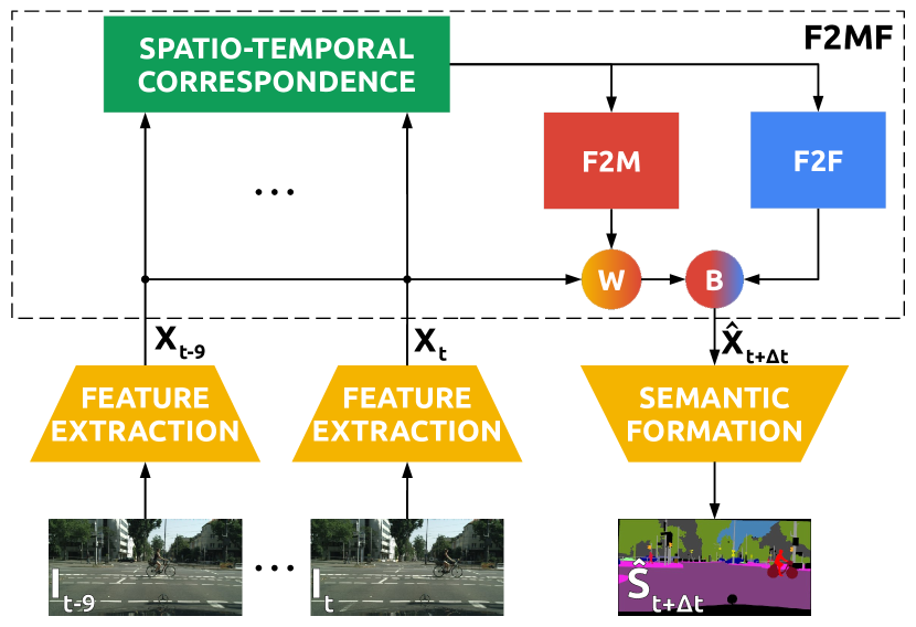
Figure 1: Overview of the proposed F2MF forecasting. Low-resolution features $\mathbf{X}_{\tau}$ are extracted from observed RGB images $\mathrm{I}_{\tau}$, $\tau\in\{t-9,t-6,t-3,t\}$ by a pre-trained recognition module. The features are enriched with their spatio-temporal correlations and forwarded to F2M and F2F modules which specialize for forecasting previously observed and novel scenery. The forecasted future features $\mathbf{\hat{X}}_{t+\Delta t}$ are a blend (B) of F2M and F2F outputs. Dense semantic predictions $\mathbf{\hat{S}}_{t+\Delta t}$ are finally formed throughout a pre-trained upsampling module.

Early visual forecasting methods relied on handcrafted models of scene dynamics [3]. However, this approach is prone to systematic errors due to insufficient modeling accuracy. For instance, popular camera models [4] are unable to express arbitrary lens distortions [5]. Likewise, object-level forecasting by geometric filtering [6] is vulnerable to propagation of detection and association errors. Consequently, recent work attempts to implicitly capture the laws of scene dynamics through deep learning in video [7]. This can be carried out by forecasting either future RGB frames [8, 9], or the corresponding semantic content [10, 11, 12].

Semantic forecasting is an appealing approach since decision-making systems mainly care about the content of future scenes rather than about their appearance [13]. Empirical evidence indicates that direct semantic foreasting performs much better than inferring from a forecasted RGB frame, while requiring significantly less computational effort [11]. Intuition suggests similar conclusions. It seems appropriate to first figure out what is going to happen at an abstract level before moving on to RGB pixels and the associated details of lighting, reflectance and surface normals. Indeed, it appears that semantic forecasting should be a prerequisite for RGB forecasting rather than vice versa.

There are multiple approaches for expressing semantic forecasting. Semantics-to-semantics forecasting (S2S) maps observed semantic maps into their future counterparts [11]. Motion-to-motion forecasting (M2M) receives the optical flow between observed images and produces the optical flow between the future image and the last observed image [14]. Finally, feature-to-feature forecasting (F2F) operates on abstract convolutional features [12]. There are several advantages of F2F forecasting with respect to the remaining two approaches. In comparison with S2S, it offers better spatio-temporal correspondence, more expressive features, and task-agnosticism. In comparison with M2M, it offers semantic reasoning and in-painting the novel scenery.

This paper builds on previous feature-level forecasting approaches [12, 15] and enriches them with the following contributions. We propose F2M forecasting (feature-to-motion) which expresses future features by warping their current counterparts throughout a dense deformation field. This formulation expresses feature-level forecasting as a causal relationship between the past and the future. However, F2M forecasting is unable to predict emergence of novel scenery. Hence, we finally propose F2MF forecasting (feature-to-motion-and-feature) by blending F2M and F2F with densely regressed weight factors as illustrated in Figure 1. This allows our method to foresee emergence of unobserved scenery, and to exploit that information for decoupling variation due to novelty from variation due to motion. We account for geometric nature of our task by leveraging spatio-temporal correlation coefficients and deformable convolutions. We show that dense semantic forecasting can be expressed in terms of the most compressed representation of the single-frame model, and that such organization can lead to competitive accuracy. The resulting generalization performance surpasses the state-of-the-art by a wide margin. Our method is very-well suited for real-time implementation due to low computational overhead with respect to single-frame prediction [16]. The method can be adapted for other dense prediction tasks, which we explain next.

In addition to contributions from previous conference accounts [16, 17], here we extend F2MF forecasting with two new single-frame architectures [1, 2], and show that single-level forecasting can preserve instance-related information. Thus, this is the first forecasting method that can be applied to three dense prediction tasks: semantic segmentation, instance-level segmentation, and panoptic segmentation. We note that transition towards instance-aware tasks is not trivial since the corresponding metrics (AP and PQ) aggregate instance-level instead of pixel-level recognition quality. Hence, correct recognition of small objects becomes much more important than in semantic segmentation. This paper also presents computational advantages of our method by comparing its complexity with other dense semantic forecasting approaches. Finally, it demonstrates that our method is able to generalize over different cameras, resolutions and framerates, as well as to produce longer-term forecasts in an autoregressive manner.

II Related Work

Semantic forecasting anticipates semantic contents of an unobserved future image. Conceptually, this task can be factorized into RGB forecasting [8] and semantic prediction in the forecasted image. However, we prefer to carry it out as a single processing step [11] due to advantages stated in the introduction. In particular, we consider forecasting three dense prediction tasks: semantic segmentation [18], instance segmentation [1] and panoptic segmentation [2]. Our method warps features from observed images into their future positions, which makes it related to optical flow [19]. Our work is most related to previous dense semantic forecasting approaches F2F [12] and M2M [14].

II-A Optical flow

Optical flow is a dense 2D-motion field between neighbouring image frames $\mathrm{I}_{t}$ and $\mathrm{I}_{t+1}$. A future image $\mathrm{I}_{t+1}$ can be approximated either by forward warping $\mathrm{I}_{t}$ with the forward flow $\mathbf{f}_{t}^{\mathrm{t+1}}$= $\textrm{flow}(\mathrm{I}_{t},\mathrm{I}_{t+1})$, or by backward warping it with the backward flow $\mathbf{f}_{t+1}^{t}$= $\textrm{flow}(\mathrm{I}_{t+1},\mathrm{I}_{t})$ [20]:

$$\mathrm{I}_{t+1}\approx\mathrm{warp\_fw}(\mathrm{I_{t}},\mathbf{f}_{t}^{t+1})\approx\mathrm{warp\_bw}(\mathrm{I_{t}},\mathbf{f}_{t+1}^{t})$$ (1)

The approximate equality reminds us that bijective mapping can not be established due to occlusions and disocclusions.

Recent optical flow methods leverage deep convolutional models [21, 22] due to capability to guess motion where the correspondence is absent or ambiguous. These approaches exploit explicit 2D correlation across the local neighbourhood [21], and local embeddings which act as a correspondence metric [23]. Our method is especially related to self-supervised approaches [19] since they learn to reconstruct optical flow without any groundtruth information.

II-B RGB forecasting

RGB forecasting is also known as video prediction [8]. The task is to predict one or more future video frames given a few recently observed frames of the same scene [7]. This is especially interesting due to opportunity for self-supervised representation learning on practically unlimited data.

Mathieu et al. [8] express RGB forecasting as image generation with a multiscale adversarial network. Vukotic et al. [24] embed the desired temporal offset in the latent representation of the observed scenery. Reda et al. [25] warp observed frames by applying a regressed kernel at the location determined by the forecasted flow.

Some works generate video from still images by warping the image with forecasted flow [26, 27]. Our approach forecasts multiple flows which warp multiple previous features towards a single future feature tensor. This allows to resolve some disocclusions by warping from a suitable past image.

Some works decompose RGB forecasting into reconstruction from the past and in-painting the novel scenery [26, 28, 9]. Their forecast includes the future warp and the respective disocclusion map. The past frame is first warped with forecasted flow, and then the disocclusions are filled by in-painting. This setup is conceptually similar to the proposed F2MF approach, however there are two important differences as follows. First, we exploit spatio-temporal correlation features and deformable convolutions. Second, we perform the forecast on heavily subsampled (16$\times$ or 32$\times)$ abstract features instead of pixels. This allows our method to operate on megapixel images and to achieve state-of-the-art accuracy in semantic forecasting while incurring only a modest computational overhead with respect to single-frame prediction.

II-C Dense semantic prediction

Several computer vision tasks address scene understanding at the pixel level. Semantic segmentation [18] assigns each pixel to a suitable semantic class. This includes stuff classes such as road or vegetation, as well as object classes such as person or bicycle. Instance segmentation [1] detects instances of object classes and associates them with the respective image regions. Panoptic segmentation [2] subsumes the previous two tasks by assigning pixels both the semantic class and the instance index. Today, all these tasks are solved by fully convolutional models for dense prediction.

Several succesful architectures for dense semantic prediction have an asymetric hourglass-shaped structure consisting of the recognition backbone and a lean upsampling datapath [29, 30, 2]. The recognition backbone usually corresponds to a fully-convolutional portion of a model designed for image classification. The role of this component is to convert the input image into a subsampled latent representation. Most authors exploit knowledge transfer from ImageNet since image-wide supervision requires much less effort than dense semantic supervision. The upsampling datapath recovers dense semantic predictions by blending semantics of deep features with location accuracy of their shallow counterparts. The blending is usually implemented by means of skip-connections from the backbone towards the upsampling path. Empirical studies show advantages of asymetric designs which complement deep and thick recognition with shallow and thin upsampling [31]. This suggests that recognition requires much more capacity than guessing the borders when rough semantics is known.

II-D Forecasting at the level of semantic predictions (S2S)

Luc et al. [11] were the first to propose direct semantic forecasting. Their S2S model maps past semantic segmentations into the future semantic segmentation. Bhattacharyya et al. [32] try to account for multimodal future with variational inference based on MC dropout, while conditioning the forecast on measurements from the vehicle odometer. Rochan et al. [33] formulate the forecasting in a recurrent fashion with shared parameters between each two frames. Chen et al. [34] improve their work by leveraging deformable convolutions and enforcing temporal consistency between neighbouring feature tensors. Their attention-based blending is related to forward warping based on pairwise correlation features [17]. However, the forecasting accuracy of these approaches is considerably lower than in our ResNet-18 experiments despite greater forecasting capacity and better single-frame performance. This suggests that ease of correspondence and avoiding error propagation may be important for successful forecasting. Concurrent work [35] forecasts panoptic segmentation by separately regressing things and stuff from previous predictions.

II-E Flow-based forecasting (M2M)

Direct semantic forecasting requires a lot of training data due to necessity to learn all motion patterns one by one. This can be improved by allowing the forecasting model to access geometric features which reflect 2D motion in the image plane [36]. Further development of that idea brings us to warping the last dense prediction according to forecasted optical flow. A prominent instance of this approach can be succinctly described as motion-to-motion (M2M) forecasting since it receives optical flows from three observed frames and produces the future optical flow. The corresponding implementation based on convolutional LSTM had achieved state-of-the-art semantic forecasting accuracy prior to our work [14]. This approach is related to our F2M module which also forecasts by warping with regressed flow. However, our F2M module operates on abstract convolutional features, and does not require external computational resources and additional supervision for training and evaluating the flow model. Our approach discourages error propagation due to end-to-end training and implies very efficient inference due to subsampled resolution and feature sharing between motion reconstruction and dense recognition. Additionally, we take into account features from all past four frames instead of relying only on the last prediction. This allows our F2M module to detect complex disocclusion patterns and simply copy from the past where possible. Further, our module has access to raw semantic features which are complementary to flow patterns [37], and often strongly correlated with future motion (consider e.g. cars vs pedestrians). Finally, we complement our F2M module with pure recognition-based F2F forecasting which outperforms F2M on previously unobserved scenery.

II-F Feature-level forecasting (F2F)

Feature-to-feature (F2F) forecasting maps past features to their future counterparts. The first F2F approach operated on image-wide features from a fully connected AlexNet layer [38]. Luc et al. [12] propose dense F2F forecasting by regressing all features along the FPN-style [29] upsampling path. Further work [15, 39] improves by using a convolutional LSTM module at each level of the feature pyramid, and proposing inter-level connections for context sharing. However, forecasting at fine resolution is computationally expensive [40]. Hence, we propose single-level forecasting of the coarsest features [16, 41]. Such aproach is advantageous due to small inter-frame displacements, rich contextual information and small computational footprint [16]. It also has an intuitive appeal of prioritizing the big picture before moving on to the fine details. Most recent work [42] follows and extends our idea of single-level feature forecasting. They introduce a variational autoencoder which provides a compressed representation of a multi-level feature pyramid. After the forecasting, this representation is decoded into tensors of the FPN style decoder.

Vora et al. [43] formulate feature-level forecasting as reprojection of reconstructed features to the forecasted future ego-location. However, such approach underperforms in presence of (dis-)occlusions and large changes of perspective. Additionally, it makes it difficult to account for independent motion of moving objects. Large empirical advantage of our method suggests that optimal forecasting performance requires a careful balance between reconstruction and recognition, as well as that explicit 3D reasoning may bring minor benefits.

II-G Semantic forecasting in video

Dense semantic forecasting has been used to increase the level of supervision in partially labeled video [44]. This could be especially useful when only few [45] or weak [46] labels are available. Semantic forecasting can improve inference in video by alleviating disturbances due to noisy input [3]. Learned object dynamics could especially improve few-shot approaches which rely on inference-time optimization [47].

III Dense semantic forecasting with F2MF

We present a novel forecasting approach which combines standard feature-level forecasting (F2F) with its regularized variant (F2M) which warps past representations into the future. Fig. 2 illustrates the structure of the proposed joint model. On input, we receive $T$=$4$ past feature tensors $\mathbf{X}_{t-9}$, $\mathbf{X}_{t-6}$, $\mathbf{X}_{t-3}$, $\mathbf{X}_{t}$ ($\mathbf{X}_{\mathtt{t-9:t:3}}$ for short) extracted with the front end of the desired single-frame model for dense semantic prediction. Our F2MF model maps the past features into the future feature tensor $\mathbf{\hat{X}}_{t+\Delta t}$. This tensor is transformed to semantic predictions $\mathbf{\hat{S}}_{t+\Delta t}$ throughout the back end of the chosen single-frame model as shown in Fig. 1. Note that $\Delta t$ denotes the temporal offset between the last observed frame and our forecast.

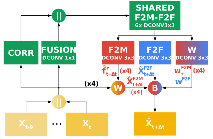
Figure 2: Details of F2MF forecasting. F2M and F2F modules receive a processed concatenation ($||$) of features from observed frames ($\mathbf{X}_{t-9:t:3}$), and their spatio-temporal correlation coefficients. The F2M module regresses future feature flow which warps (W) past features into their future locations. The F2F module forecasts the future features directly. The compound forecast $\mathbf{X}_{t+\Delta t}$ is a weighted blend (B) of F2M and F2F forecasts.

F2MF forecasting proceeds as follows. Input features are concatenated across the semantic dimension and fused with a single convolutional layer in order to reduce the number of channels. In parallel, the correlation module computes pairwise correlation coefficients across a local neighborhood. The fused representation is concatenated with the correlation features. The result is further processed through six convolutional layers in order to recover the shared representation for F2M and F2F forecasting. The weight module (block W in Fig. 2) outputs five feature maps: $w^{\text{F2M}}_{t-9},w^{\text{F2M}}_{t-6},w^{\text{F2M}}_{t-3},w^{\text{F2M}}_{t}$ and $w^{\textrm{F2F}}$. The four maps $[w^{\textrm{F2M}}_{\tau}]$, $\tau\in\{t-9:t:3\}$ represent contributions of the four past feature tensors in the F2M forecast. The fifth map $w^{\textrm{F2F}}$ represents the contribution of the F2F head in the compound forecast. All convolutional layers are implemented as BN-ReLU-dconv, where dconv stands for deformable convolution [48].

III-A F2M module

The F2M module assumes that the future can be explained as a geometrical transformation of the observed past. Therefore, it outputs a dense field of motion vectors $\mathbf{\hat{f}}_{t+\Delta t}^{\tau}$ for each of the T=4 input feature tensors $\mathbf{X}_{\tau}$, $\tau\in\{t-9,t-6,t-3,t\}$. The future tensors ${\hat{X}}^{(\tau)}_{t+\Delta t}$ are estimated by backward warping [20] the corresponding input features $\mathbf{X}_{\tau}$ with the regressed flow $\mathbf{\hat{f}}_{t+\Delta t}^{\tau}$. The resulting warped tensors are subsequently blended with regressed weights which we activate with per-pixel softmax. Thus, the F2M forecast is a weighted sum of warped features from the observed images:

$$\quad\mathbf{\hat{X}}^{(\tau)}_{t+\Delta t} =\mathrm{warp\_bw}(\mathbf{X}_{\tau},\mathbf{\hat{f}}_{t+\Delta t}^{\tau})$$ (2)

$$\mathbf{\hat{X}}_{t+\Delta t}^{\mathrm{F2M}} =\sum_{\tau}\mathbf{\alpha}_{\tau}\cdot\mathbf{\hat{X}}^{(\tau)}_{t+\Delta t}$$ (3)

$$\bm{\alpha} =\textrm{softmax}([w^{\textrm{F2M}}_{\tau}]_{\tau\in\{t-9:t:3\}})\;.$$ (4)

This allows the F2M module to choose the most suitable previous image for forecasting a particular region. Such opportunity is particularly beneficial in some occlusion patterns as we illustrate in Fig. 10.

However, the assumption that the future can be reconstructed from the past is only partially true, since the future often brings unpredictable novelty. Additionally, sometimes the correspondence will be hard to determine due to large ego-motion and changes in perspective. Consequently, some parts of the scene are going to be particularly hard to forecast by simple warping from the past. Accurate forecasting of such regions will require imagination ability as we describe next.

III-B F2F module

The F2F module directly regresses future features $\mathbf{\hat{X}}_{t+\Delta t}^{\mathrm{F2F}}$ from the shared representation. It consists of a single BN-ReLU-dconv unit, where the number of output feature maps is the same as in a single past feature tensor. As it is not bound to reconstruction from the past, it has a chance to in-paint the features in novel regions. This is similar to some previous [12], and concurrent work [15, 41], however there are three important differences. First, we aim at single-level F2F forecasting. Second, we use deformable convolutions. Third, our F2F module has access to spatio-temporal correlation features which relieve the need to learn correspondence from scratch. Our experiments show clear advantage of these novelties. The contribution of correlation features suggests that correspondence is not easily learned on existing datasets.

III-C Compound F2MF forecasting

We hypothesize that F2M and F2F forecasting might be complementary and that their combination might lead to improved accuracy. Consequently, our F2MF module formulates future features as a weighted average of the F2M and F2F forecasts (as before, $\tau\in\{t-9:t:3\}$):

$$\mathbf{\hat{X}}_{t+\Delta t}^{\mathrm{F2MF}} =\beta^{\textrm{F2F}}\cdot\mathbf{\hat{X}}_{t+\Delta t}^{\mathrm{F2F}}+\sum_{\tau}\beta^{\textrm{F2M}}_{\tau}\cdot\mathbf{\hat{X}}_{t+\Delta t}^{\mathrm{(\tau)}}$$ (5)

$$\bm{\beta} =[\beta^{\textrm{F2F}}]\mathbin{\|}[\beta^{\textrm{F2M}}_{\tau}]=\textrm{softmax}([w^{\textrm{F2F}}]\mathbin{\|}[w^{\textrm{F2M}}_{\tau}])\;.$$ (6)

This formulation encourages specialization of the F2F module for the novel parts of the scene. It also relaxes the penalty of the F2M module in such regions and allows it to focus on parts where correspondence can be established. Nevertheless, this kind of separation might weaken the learning signals within the two individual modules. Consequently, we propose to train F2MF forecasting with three loss terms. The main loss $\mathcal{L}_{\mathrm{F2MF}}$ involves the F2MF forecast (5). The two auxiliary losses $\mathcal{L}_{\mathrm{F2F}}$ and $\mathcal{L}_{\mathrm{F2M}}$ affect the corresponding outputs $\mathbf{\hat{X}}_{t+\Delta t}^{\mathrm{F2F}}$ and $\mathbf{\hat{X}}_{t+\Delta t}^{\mathrm{F2M}}$. All three losses are formulated as mean squared L2 distance between the forecast and actual features computed with the single-frame model in the future frame. Consequently, the model can be trained with self-supervision on unlabeled video.

III-D Correlation module

Our correlation module determines spatio-temporal correspondence between neighbouring frames. On input, it receives convolutional features $\mathbf{X}_{\mathtt{t-9:t:3}}$ in the form of a T $\times$ C $\times$ H $\times$ W tensor. On output, it produces spatio-temporal correlation coefficients across a d$\times$d neighborhood for each of the T$-$1 pairs of neigbouring frames.

The module first embeds features from all time instants into a space with enhanced metric properties by a shared 3$\times$3$\times$C’ convolution (C’=128). We hypothesize that this mapping might recover distinguishing information which is not needed for single-frame inference. Subsequently, we construct our metric embedding by normalizing C’-dimensional features to unit norm so that cosine similarity becomes dot product. This results in a T$\times$C’$\times$H$\times$W metric embedding $\mathbf{F}$. Finally, we produce $d^{2}$ correspondence maps between features at time $\tau$ and their counterparts at $\tau-3$ within the local $d\times d$ neighborhood for each $\tau\in\{t-6,t-3,t\}$. We usually set $d=9$. We denote the value of the correlation tensor $\mathbf{C}^{\tau}$ at location $\mathbf{q}$ and feature map $ud+v$ as $\mathbf{C}^{\tau}_{ud+v,\mathbf{q}}$. This value corresponds to a dot product between a metric feature at time $\tau$ and location $\textbf{q}\in\mathcal{D}(\mathbf{F})$, and its counterpart at time $\tau-3$ and location $\textbf{q}+(u,v)$ where $u,v\in 0\,..\,d-1$ [21]:

$$\mathbf{C}^{\tau}_{ud+v,\mathbf{q}}=\mathbf{F}^{\tau\top}_{\mathbf{q}}\mathbf{F}^{\tau-3}_{\mathbf{q}+[u-\frac{d}{2},v-\frac{d}{2}]},\mathrm{where}\ u\mathrm{,}v\in[0\,..\,d).$$ (7)

Each of the $d^{2}$ feature maps of $\mathbf{C}^{\tau}$ can be computed by elementwise multiplication of $\mathbf{F}^{\tau}$ and shifted $\mathbf{F}^{\tau-3}$ followed by channel reduction. Please note that $\mathcal{D}(\mathbf{F})$ denotes the set of all spatial locations in $\mathbf{F}$: $\mathcal{D}(\mathbf{F})$= {1..H-1}$\times${1..W-1}.

III-E Application to popular single-frame models

Figure 1 suggests that our F2MF approach can be applied to a variety of single-frame architectures for dense semantic forecasting. The pipeline consists of three processing steps. First, the front end of the single-frame model extracts features from multiple past frames. Second, our F2MF module processes the present features and recovers the forecast of the future features. Finally, the back end of the single-frame model processes the forecasted features and forms the future dense semantic prediction.

Different than [12], the presented forecasting approach addresses features at only one level of abstraction [16]. We propose to forecast succinct abstract features in order to encourage the forecasting module to focus on the big picture. This approach is also advantageous since low spatial resolution makes it easier to establish spatio-temporal correspondence.

However, ladder-style architectures [30, 29] present challenges towards implementing single-level forecasting. Their skip-connections require either multi-level forecasting [12] or single-level forecasting of high-resolution features from the last upsampling module. Unfortunately, both of these options have to confront high computational complexity and large displacements. None of our experiments along these directions outperformed our single-level designs. We therefore base our experiments on single-frame architectures with a reduced number of skip connections, which leads to faster training and inference. This reduces single-frame performance on small objects, however the forecasting penalty will be contained since small objects are the hardest to forecast.

III-F Forecasting semantic segmentation

In the case of semantic segmentation we achieve our best results with custom single-frame models without any skip connections. The single-frame penalty of this design decision is around 3 percentage points (pp) mIoU on Cityscapes val. Despite this handicap, our best mid-term forecasting accuracy outperforms the state-of-the-art for more than 6 pp mIoU. Figure 3 shows that our F2MF forecasting addresses 512-dimensional features produced by the SPP module, as well as that the semantic forecast is formed by the upsampling path of the single-frame model.

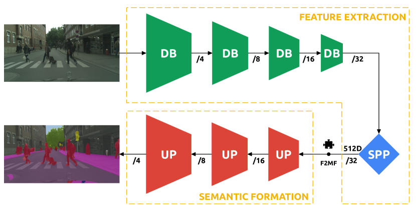
Figure 3: Details of our single-frame model for semantic segmentation. Notice the absence of skip connections from the backbone (green) towards the upsampling path (red). The black jigsaw symbol indicates the feature tensor which we use for F2MF forecasting. Feature extraction and semantic formation modules are in correspondence with Fig. 1.

III-G Forecasting instance segmentation

In the case of instance segmentation, we choose a third-party implementation of a Mask R-CNN without skip connections [1]. The single-frame penalty of this design decision is around 1 pp AP COCO and 2.7 pp AP50 on Cityscapes val. Despite this handicap, our model performs favourably with respect to the state-of-the-art. Figure 4 shows that our F2MF forecasting addresses 1024-dimensional features produced by the second-to-last residual block of the ResNet-50 backbone. Subsequently, the RPN head extracts object candidates from the forecasted features. Instance segmentations are obtained by processing each object candidate with the last residual block and the two Mask R-CNN heads. Future semantics is formed by resizing the inferred instance segmentations to input resolution.

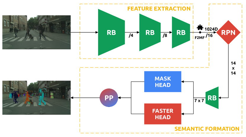
Figure 4: Details of a single-frame model which we use in instance segmentation experiments. This is a Mask R-CNN model [1] which generates proposals and detections at 16$\times$ subsampled resolution. The black jigsaw indicates the feature tensor which we use for F2MF forecasting. Feature extraction and semantic formation modules are in correspondence with Fig. 1.

III-H Forecasting panoptic segmentation

In the case of panoptic segmentation, we train a custom Panoptic DeepLab model [2] with only one skip connection. The single-frame penalty of this design decision is around 2.3 pp PQ on Cityscapes val. Figure 5 shows that our F2MF forecasting addresses 1024-dimensional features produced by the second-to-last residual block of the ResNet-50 backbone. Subsequently, the forecasted features are processed by the last residual block and by the two upsampling paths. Future semantics is finally formed by postprocessing object centers and per-pixel semantic information.

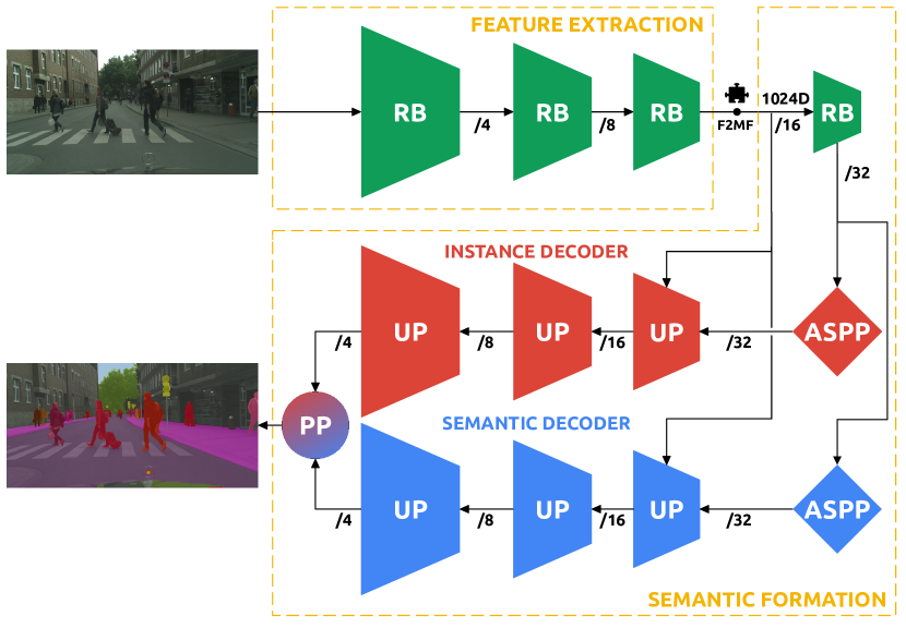
Figure 5: The adopted single-frame panoptic model is custom Panoptic DeepLab [2] with only one skip connection. This allows us to apply single-level forecasting to the feature tensor produced by the penultimate residual block, as indicated by the jigsaw symbol. Feature extraction and semantic formation modules are in correspondence with Fig. 1.

IV Experiments

We train our method on Cityscapes train [49], and evaluate on Cityscapes val and test and CamVid test. We consider short-term and mid-term forecasting experiments which target $\Delta t$=3 and $\Delta t$=9 time-steps into the future (180 and 540 ms respectively) [11]. We estimate the forecasting performance by computing the usual dense prediction metrics in the future frame. We use mean intersection over union (mIoU) for semantic segmentation, COCO average precision (AP) for instance segmentation, as well as panoptic, segmentation and recognition quality (PQ, SQ, RQ) for panoptic segmentation.

Our training procedure involves several separate steps. First, the backbone of a single-frame model is pretrained on ImageNet. Second, we train the single-frame model on labeled images in the task-specific setup. Finally, we train the forecasting module on unlabeled images to map the past features to their future counterparts with MSE loss. We extract all training features (both the past and the future) by applying the single-frame model to the corresponding video frames. Note that the forecasting module does not require any annotations in spite of being trained in a supervised fashion.

We train our model for 160 epochs with ADAM [50] optimizer and early stopping. We set the initial learning rate to $4\cdot 10^{-4}$ and reduce it to $10^{-7}$ through cosine annealing. We implement our model in Pytorch. Training with cached features takes 12 hours on a single GTX1080Ti. Training with online data augmentation requires 2 days and three GPUs. During training, we normalize inputs and outputs of our F2MF model to dataset-wide zero mean and unit variance. During inference, we normalize the input and denormalize the output. This facilitates the training process and improves generalization. We set the weights of all three components of the F2MF loss to 1. Our data augmentation policy includes sliding the input tuple across the video clip and horizontal flipping. We refrain from using any auxiliary information such as vehicle odometry or depth maps.

IV-A Semantic segmentation forecasting on Cityscapes

We experiment with two single-frame models of different capacity. Both of them have an encoder-decoder architecture [51] without skip connections. The encoder corresponds to standard ImageNet classification models. The decoder consists of a spatial pyramid pooling and three upsampling modules as shown in Figure 3. The two models differ in backbone architectures and in the width of the decoder. The weaker model is based on a ResNet-18 and uses 128 feature maps along the upsampling path. It achieves 72.5% mIoU on Cityscapes val. The stronger model uses a DenseNet-121 backbone, 512 feature maps in the SPP, 256 maps in the first upsampling module, and 128 maps in the last two upsampling modules. It achieves 75.8% mIoU on Cityscapes val.

Table I shows the forecasting accuracy for semantic segmentation on Cityscapes val. The top section shows the performance of our single-frame model which we denote as oracle since our forecasting models generate predictions for unobserved frames. We also show the performance of a simple baseline approach which copies the segmentation from the last observed input frame. The middle section shows experiments from the literature [11, 12, 32, 33, 34, 14, 41, 43]. The bottom section presents performance of our F2MF models with different single-frame models and data augmentation policies. Our best model achieves state-of-the-art forecasting performance with 69.6% mIoU at short-term and 57.9% mIoU at mid-term.

TABLE I: Evaluation of our F2MF model for semantic segmentation forecasting on Cityscapes val. All denotes all classes, MO — moving objects, d.a. — data augmentation, and †— test set.

	Short term:s$\Delta t$=3			Mid term: $\Delta t$=9
Accuracy (mIoU)		All	MO		All	MO
Oracle-DN121		75.8	75.2		75.8	75.2
Oracle-RN18		72.5	71.5		72.5	71.5
Copy last (DN121)		53.3	48.7		39.1	29.7
3Dconv-F2F [41]		57.0	/		40.8	/
Dil10-S2S [11]		59.4	55.3		47.8	40.8
LSTM S2S [33]		60.1	/		/	/
Mask-F2F [12]		/	61.2		/	41.2
FeatReproj3D [43]		61.5	/		45.4	/
Bayesian S2S [32]		65.1	/		51.2	/
LSTM AM S2S [34]		65.8	/		51.3	/
LSTM M2M [14]		67.1	65.1		51.5	46.3
F2MF-RN18 w/o d.a.		66.9	65.6		55.9	52.4
F2MF-DN121 w/o d.a.		68.7	66.8		56.8	53.1
F2MF-DN121 w/ d.a.		69.6	67.7		57.9	54.6
F2MF-DN121 w/ d.a. †		70.2	68.7		59.1	56.3

The table suggests that better single-frame model leads to better forecasting, however the single-frame advantage decreases in the forecasting setup. The difference in the oracle performance is 3.3 mIoU points, but it drops to 1.8 mIoU points at short-term, and 0.9 mIoU points in mid-term forecasting. We retrain our best model on trainval and submit the test set predictions to the online benchmark. This resulted in 70.2% mIoU at short-term and 59.1% mIoU at mid-term forecasting. This suggests that our performance in Table I has not been artificially improved through validation experiments on Cityscapes val.

IV-B Instance segmentation forecasting on Cityscapes

Table II presents the accuracy of our forecasting approach on the instance segmentation task and compares it to the related work on Cityscapes val. As in the case of semantic segmentation, we use single-level forecasting in order to reduce the memory footprint and to improve the speed of training. We demonstrate that our approach is a plug-in solution for any dense-prediction model without skip connections, by experimenting on a public Mask R-CNN model [52] which we do not customize (cf. Fig. 4). The chosen model (R50-C4) attaches the RPN prediction head to $16\times$ subsampled features produced by the penultimate residual block of ResNet-50. We compare our approach with previous forecasting approaches [12, 15, 39] which use Mask R-CNN with FPN upsampling [29]. The two previous approaches require forecasting all four levels of the feature pyramid. The table shows that our approach achieves the best short-term accuracy in spite of considerably weaker oracle and significantly lower computational complexity. The F2F-Corr baseline ablates the F2M module from our design. The resulting performance reveals a significant contribution of F2M forecasting in the case of instance segmentation.

TABLE II: Instance segmentation forecasting on Cityscapes val.

	Short term: $\Delta t$=3			Mid term: $\Delta t$=9
		AP	AP50		AP	AP50
Oracle (ours)		36.3	63.1		36.3	63.1
Oracle FPN [12, 15, 39]		37.3	65.8		37.3	65.8
Copy last		9.6	22.9		2.2	8.1
F2F 4$\times$ [12]		19.4	39.9		7.7	19.4
ConvLSTM F2F 4$\times$ [15]		22.1	44.3		11.2	25.6
ApaNet [39]		23.2	46.1		12.9	29.2
F2F-Corr (ours)		21.2	43.3		9.4	19.2
F2MF (ours)		23.6	47.2		11.5	24.2

IV-C Panoptic segmentation forecasting on Cityscapes

Table III presents our performance on the panoptic segmentation task. Our single-frame model is a custom Panoptic Deeplab [2] with ResNet-50 backbone and a single skip connection from the backbone to the decoder/upsampling path (cf. Fig. 5). As in the case of instance segmentation, we target the features at $16\times$ subsampled resolution from the penultimate residual block. To the best of our knowledge, this is the first attempt in forecasting panoptic segmentation. The table clearly shows that our F2MF model outperforms the copy-last baseline by a large margin. Performance of the F2F-Corr baseline reveals a significant contribution of F2M forecasting in the case of panoptic segmentation.

TABLE III: Panoptic segmentation forecasting on Cityscapes val.

	Short term: $\Delta t$=3				Mid term: $\Delta t$=9
		PQ	SQ	RQ		PQ	SQ	RQ
Oracle (ours)		57.5	79.7	70.8		57.5	79.7	70.8
Oracle (PDL) [2]		59.8	80.0	73.5		59.8	80.0	73.5
Copy-last		32.3	70.9	42.4		22.3	68.1	30.2
F2F-Corr (ours)		43.3	74.4	55.5		27.5	69.7	36.0
F2MF (ours)		47.3	75.1	60.6		33.1	71.3	43.3

Tables I-III show that F2MF forecasting can be applied to three different dense semantic prediction tasks and therefore confirm that our method indeed is task-agnostic.

IV-D Qualitative results

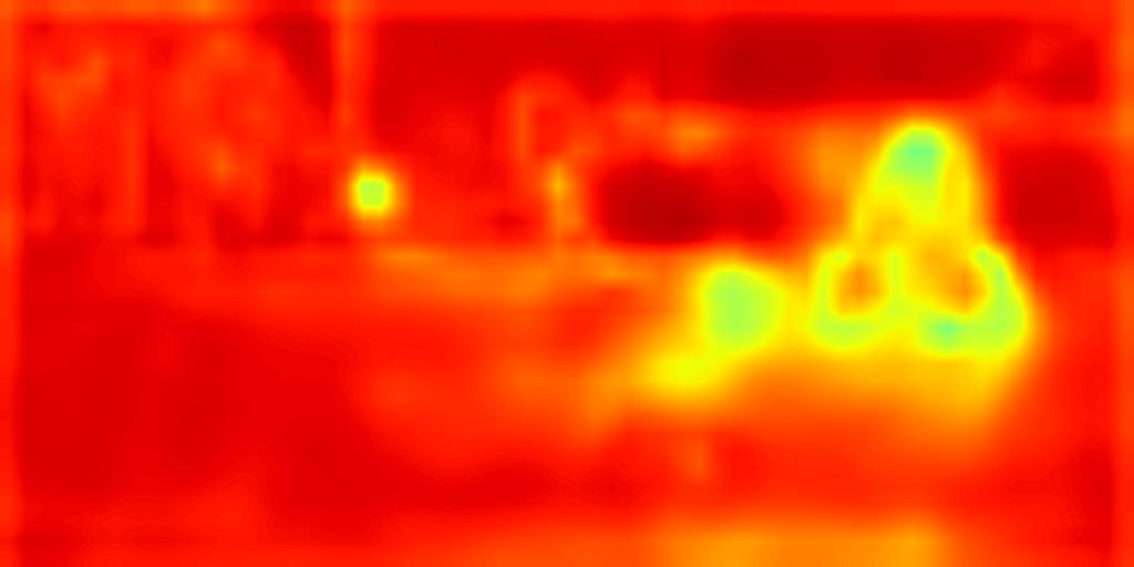
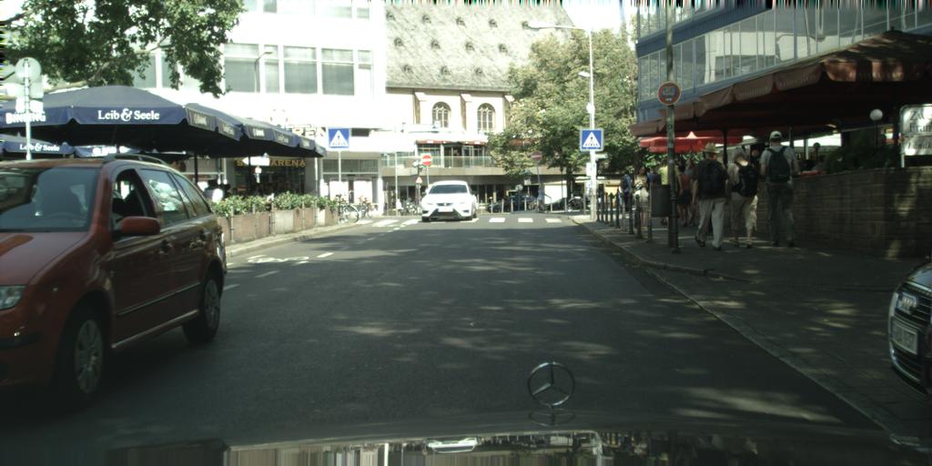
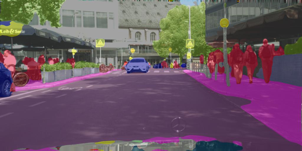
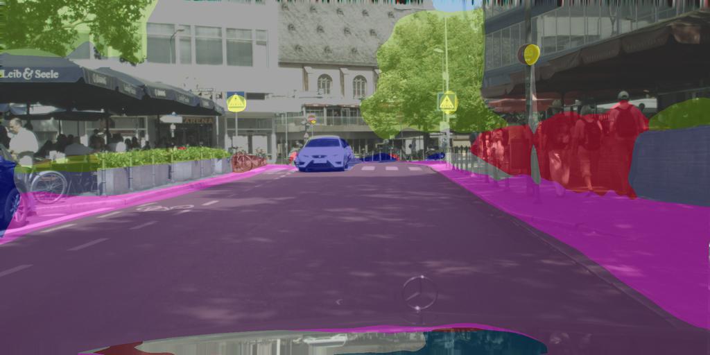
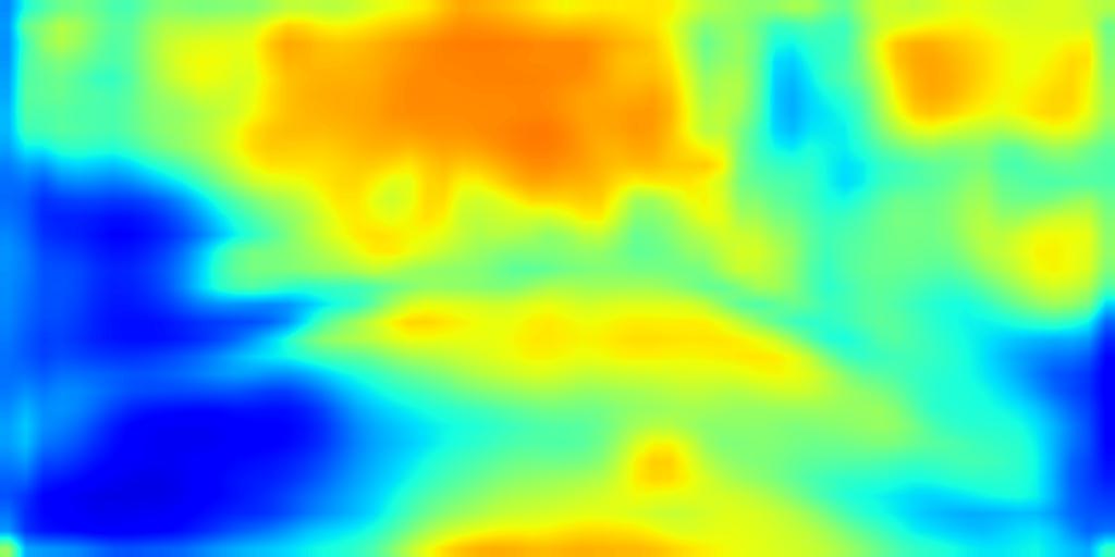
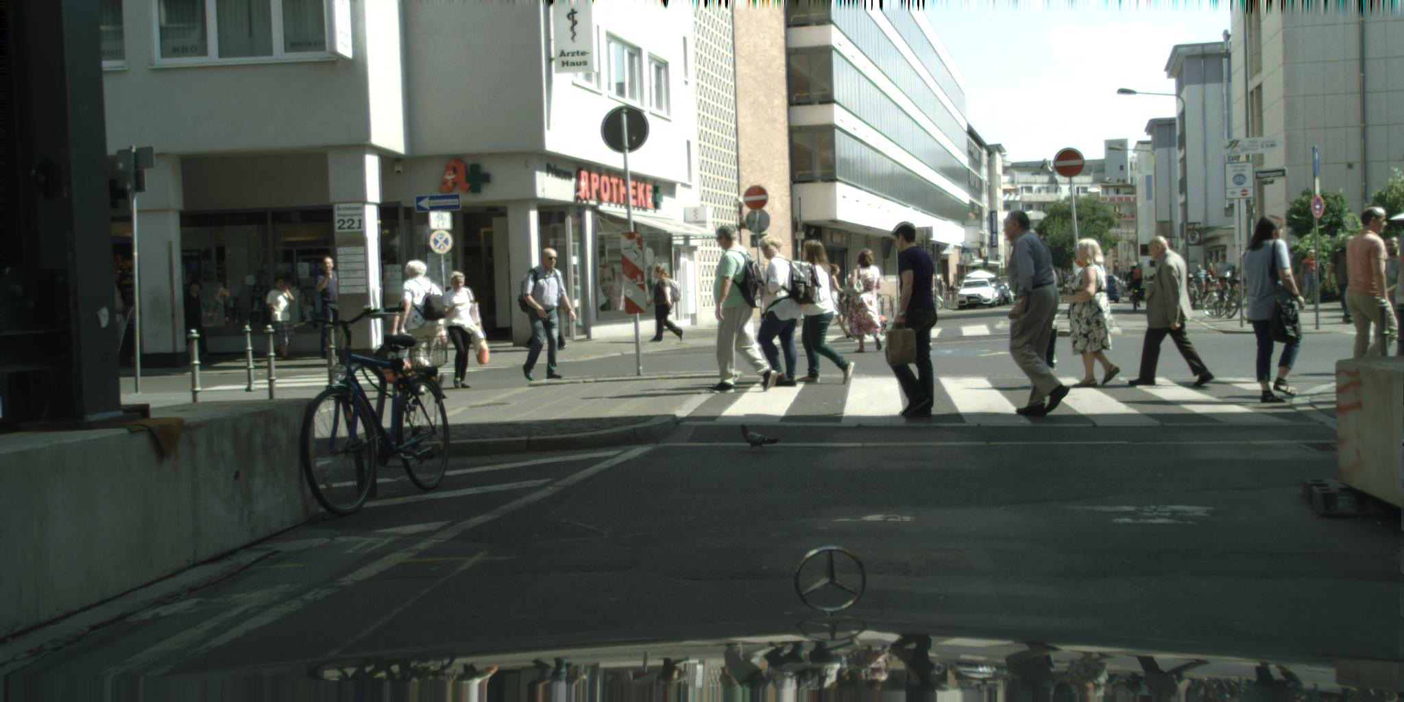
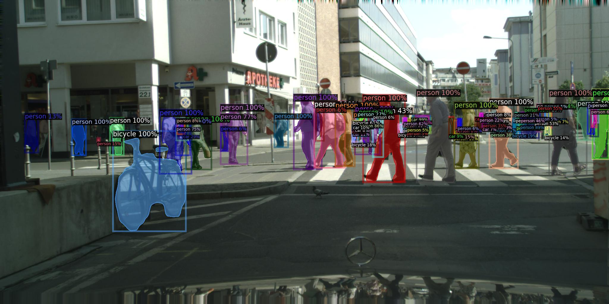
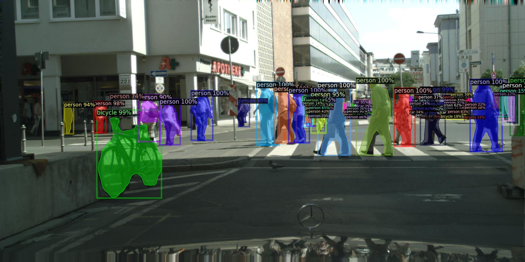
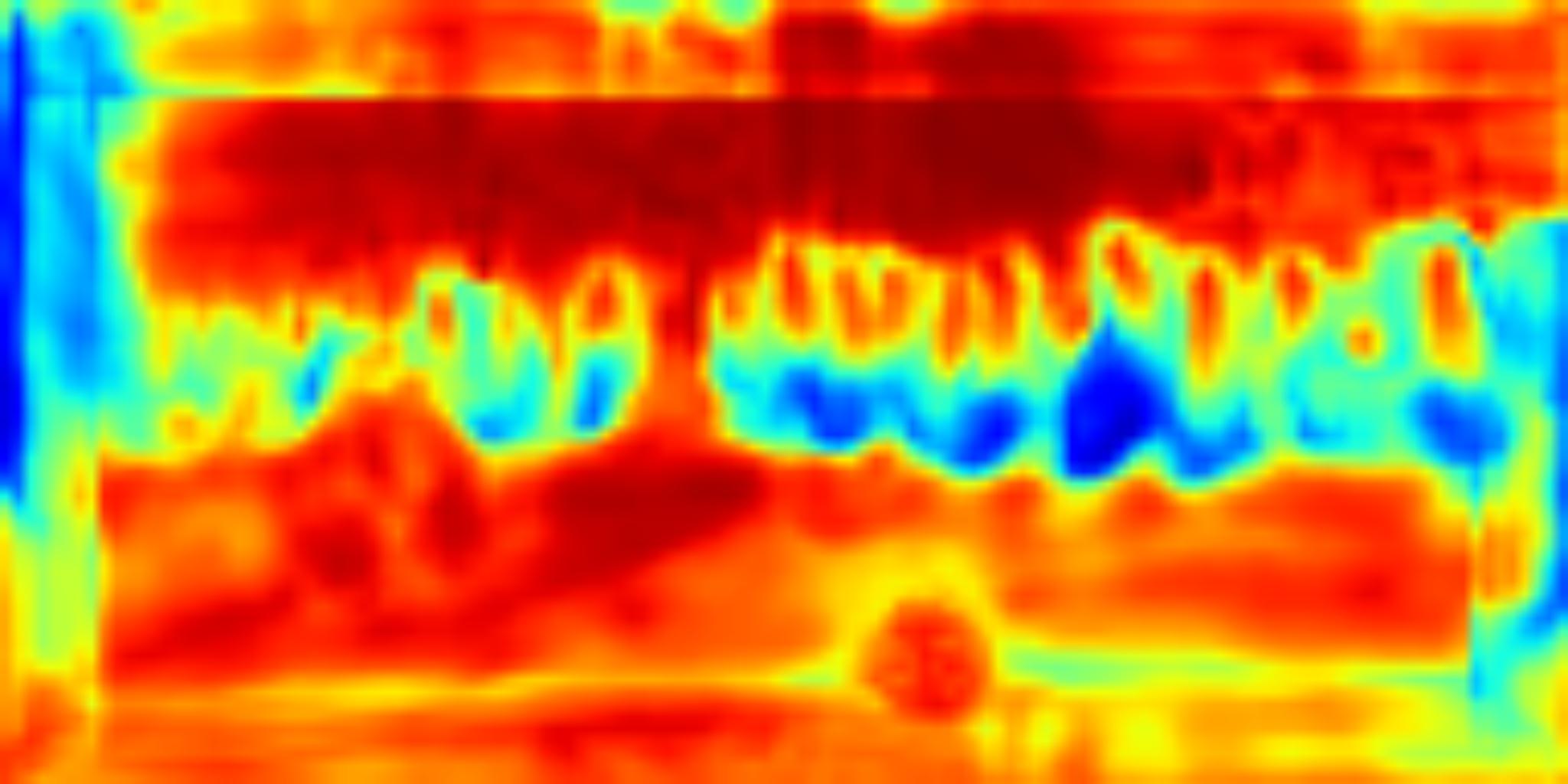
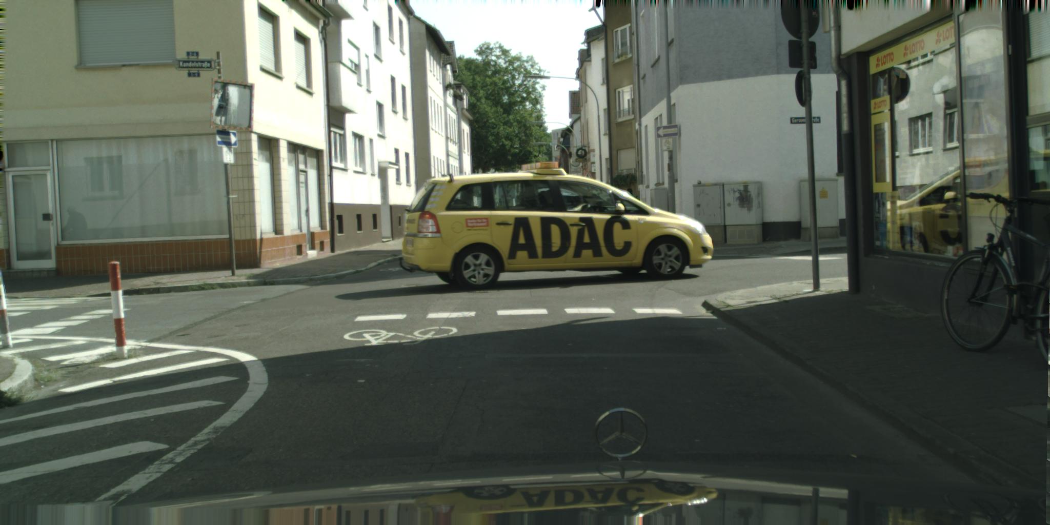
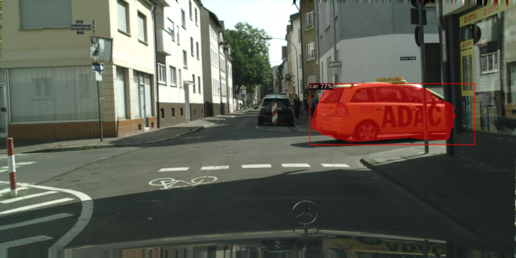
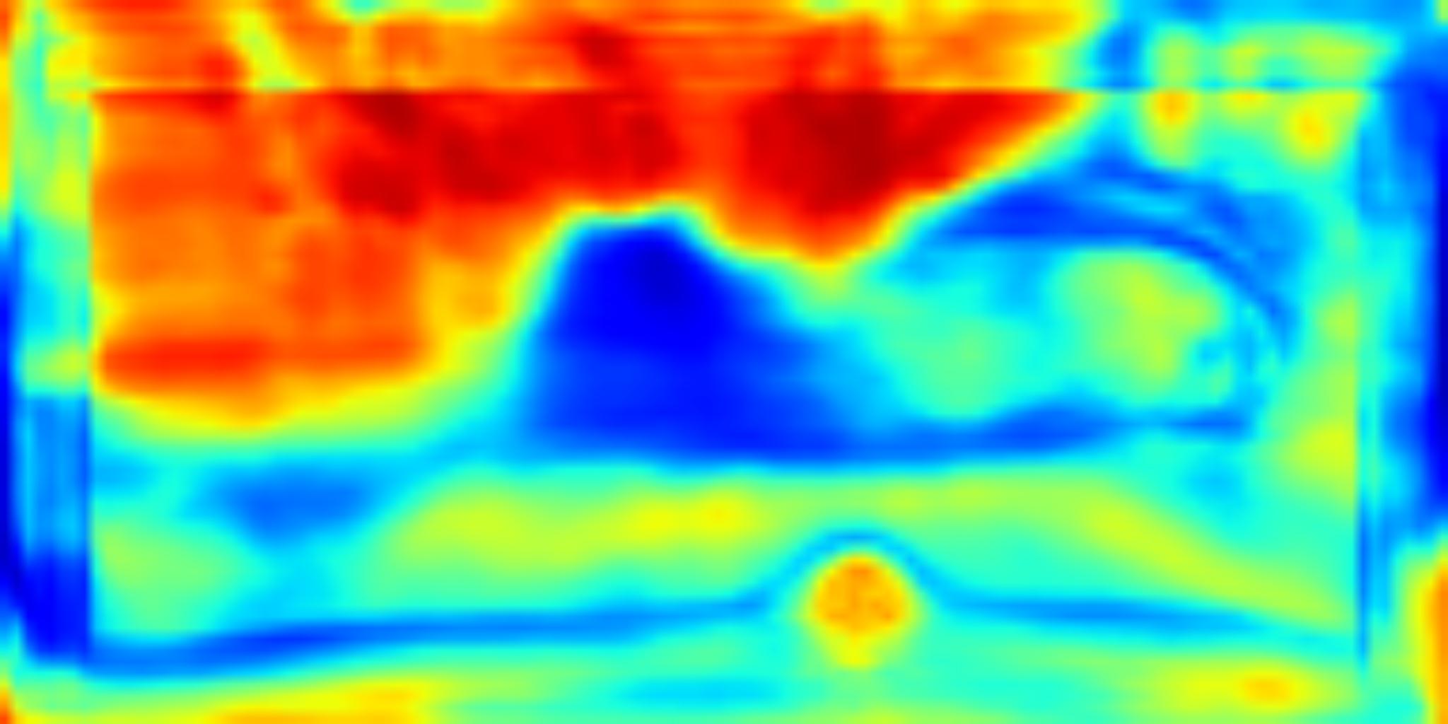
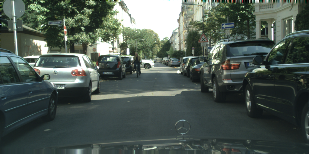
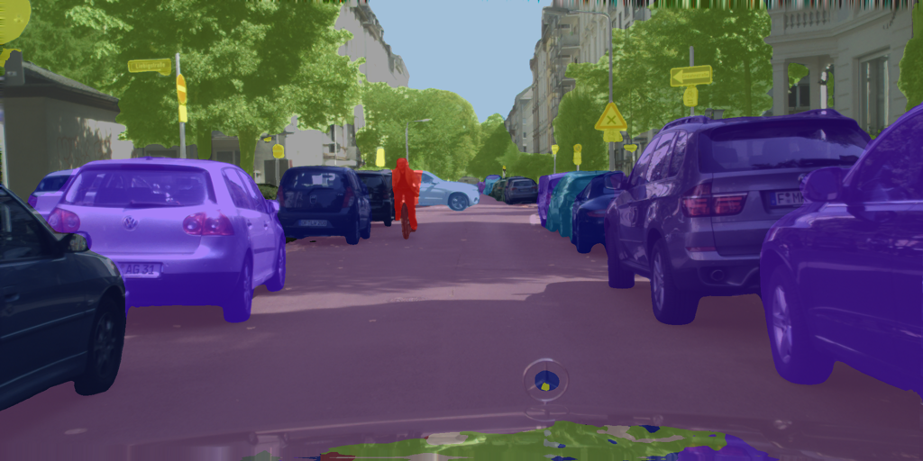
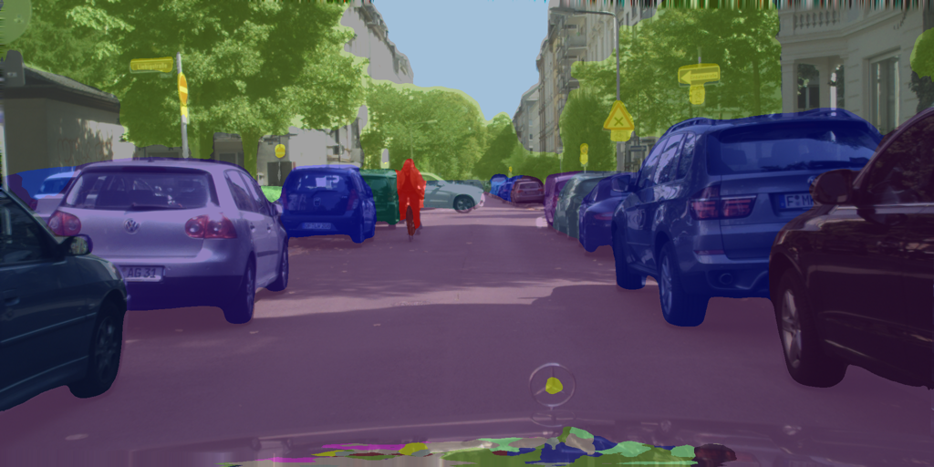
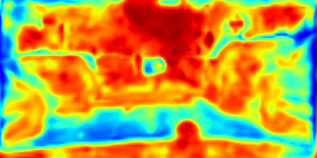
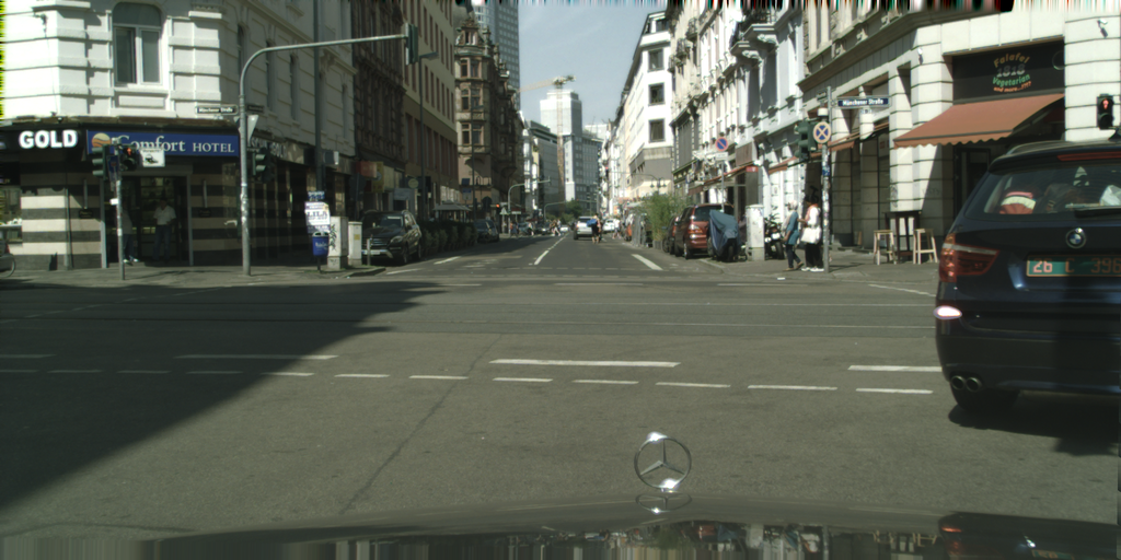
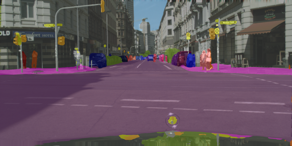
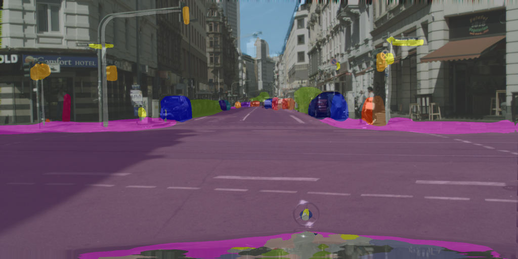
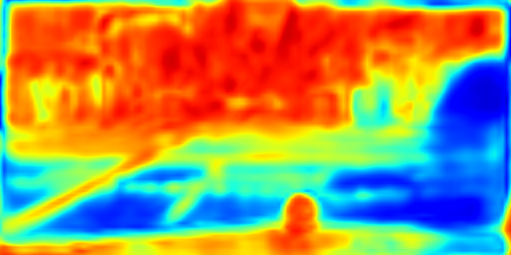
Figure 6: Qualitative results of dense semantic forecasting: semantic segmentation (top two rows), instance segmentation (middle two rows) and panoptic segmentation (bottom two rows). We show one short-term and one mid-term example for each modality. The columns show the last observed frame, oracle prediction in the future frame, F2MF forecast and the F2M heatmap.

Figure 6 visualizes our short-term and mid-term forecasts and compares them with our oracle. The columns show the last observed frame, the oracle prediction overlayed on top of the future frame, our F2MF forecast overlayed on top of the future frame, and the F2M heatmap $\beta^{\textrm{F2M}}$ = $1-\beta^{\textrm{F2F}}$ = $\sum_{\tau}\beta^{\textrm{F2M}}_{\tau}$. The red regions correspond to pixels forecasted by warping with the F2M flow while the blue regions correspond to pixels forecasted by the F2F module. The blue pixels usually correspond to unoccluded scenery which has to be imagined by the model since it was not visible in any of the observed frames. We observe that the forecasted F2M heatmaps are quite accurate in all images, which suggests that F2MF is versatile and task agnostic.

The top two rows of Figure 6 correspond to semantic segmentation. Most pixels from row 1 of this group are predicted by F2M forecasting because there is little motion in the scene. On the other hand, there is a large blue region in the bottom left of the F2M heatmap in row 2. The blue region was disoccluded by the car passing by the camera. As it was never observed before, the F2M module does not stand a chance, so the F2F module has to in-paint novel content. We observe that the prediction is sound, although it misses some of the people in behind. We also provide a video presentation of our mid-term forecasting performance on Frankfurt video.

The middle two rows illustrate instance forecasting on Cityscapes val. We observe that our model accurately predicts the future leg stance for some of the pedestrians in row 3. The F2M heatmap reveals that most human pixels are forecasted by the F2F module except for the heads which exhibit more regular motion than the bodies. Furthermore, our model correctly predicts the future position of the moving taxi in row 4. The corresponding F2M heatmap reveals that the F2F module in-paints the features in the disoccluded area. Of course, we are unable to forecast the objects behind the taxi.

The bottom two rows address panoptic forecasting on Cityscapes val. Notice that pixels corresponding to object classes are colored in different shades of the original class color. We observe that the forecasted segmentation appears sharp and accurate. Similarly as in the semantic segmentation forecasting, we observe that the F2F module is in charge for novel regions. This is best seen in the last row, where the car on the right leaves the scene and dis-occludes a large part of the background. The model correctly forecasts that the pixels behind the car correspond to buildings, sidewalk and road.

IV-E Ablation and validation study

Table IV shows validation experiments which quantify contributions from our F2F, F2M and correlation modules. We perform this study on semantic segmentation forecasting with our single-frame model based on ResNet-18. Note that we do not use data augmentation in this experiment. This enables caching the features on the SSD drive and therefore allows significantly faster training. Every model configuration presented in the table is separately trained.

First we compare F2F and F2M forecasting individually. In experiments without the correlation module, F2F outperforms F2M for 0.6 mIoU points. In experiments with the correlation module, F2F outperforms F2M for 0.7 mIoU points at short-term, and they perform equally in mid-term forecast. These results are plausible, because the F2F approach is more expressive. While F2M has to explain the future by warping past features, F2F is unconstrained and can imagine anything. Nevertheless, the compound F2MF model always outperforms any of the two single-head approaches. In a setup without the correlation module, F2MF outperforms F2M by 1.0-1.2 mIoU points, and the individual F2F by 0.4-0.6 mIoU points. In a setup with the correlation module, F2MF outperforms the F2M by 1.3-1.4 mIoU points, and the F2F by 0.6-1.4 mIoU points. These results hint that F2M and F2F are indeed complementary.

The correlation module improves the performance in all setups. It contributes 0.8 and 2.3 mIoU points in short-term and mid-term F2M forecast respectively. Likewise, the correlation module improves the F2F performance for 0.9 and 1.7 mIoU points and boosts the compound F2MF model for 1.1-2.5 mIoU points at short-term and mid-term, respectively.

TABLE IV: Ablation of correlation, F2F, and F2M on Cityscapes val. Standalone F2F and F2M models are trained independently.

Configuration (F2MF-RN18)			Short-term mIoU		Mid-term mIoU
F2F	F2M	Correlation	All	MO	All	MO
	✓		64.8	63.4	52.2	47.6
✓			65.4	64.0	52.8	48.6
✓	✓		65.8	64.7	53.4	49.7
	✓	✓	65.6	64.4	54.5	50.7
✓		✓	66.3	64.9	54.5	50.8
✓	✓	✓	66.9	65.6	55.9	52.4

We further investigate the complementary nature of the F2F and F2M approaches by comparing the accuracy of independent single-head models in stratified groups of pixels. Previous results showed that the F2F model performs slightly better in general. However, we know that predicting the future in novel regions is particularly hard for the F2M model. Therefore, we hypothesise that F2M might perform better in the previously observed scenery. We divide pixels into bins according to the $\beta^{\textrm{F2M}}$ weights as predicted by the compound F2MF model, and then show the forecasting accuracy of the two independently trained F2F and F2M models in Fig. 7. On the left y-axis we show per-bin forecasting accuracy. On the right y-axis we show the relative share of pixels in that particular bin.

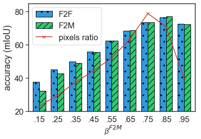
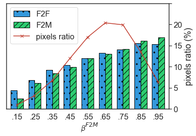
Figure 7: Histograms of F2F and F2M accuracy and overall pixel incidence over $\beta^{\textrm{F2M}}$ bins as inferred by the compound F2MF model on Cityscapes val for short-term (left) and mid-term (right) forecasting.

We show the F2M weights $\beta^{\textrm{F2M}}$ on the x-axis for each bin. The figure separately considers the short-term (left) and mid-term (right) forecasting. We observe that the pixel histogram is skewed towards higher $\beta^{\textrm{F2M}}$ values. This suggests that the F2MF model delegates the majority of the pixels to the F2M module. We also observe that this effect is less pronounced in mid-term forecast. This makes sense because we observe more novelty there. The plot also shows that F2M model performs better in pixels with higher $\beta^{\textrm{F2M}}$ values, which justifies the delegating decision from the compound model. These plots support our hypothesis that the two approaches are complementary.

Table V validates the number of input frames by exploring F2MF accuracy for different look-back windows. Models which observe only the most recent frame perform poorly as they are unable to estimate the scene dynamics with a single reference point. Note that these models do not have the correlation module because at least two frames are needed to compute spatio-temporal coefficients. Models with 2 to 5 input frames perform comparably well, while the model with 4 input frames performs the best. This confirms the suitability of the default forecasting setup [11] on Cityscapes. Please note that mid-term experiments with 5 input frames are not feasible for $\Delta$t=3 due to limited length of Cityscapes clips.

TABLE V: Validation of the number of input frames on Cityscapes.

Input frames	Short-term mIoU		Mid-term mIoU
(F2MF-RN18)	All	MO	All	MO
$\{t\}$	57.9	55.5	45.7	39.6
$\{t-3,t\}$	66.4	65.3	54.9	51.2
$\{t-6,t-3,t\}$	66.9	65.6	55.1	51.0
$\{t-9,t-6,t-3,t\}$	66.9	65.6	55.9	52.4
$\{t-12,t-9,t-6,t-3,t\}$	66.7	65.1	/	/

We have also attempted to forecast 3 and 9 steps into the future by observing input frames with stride 2 ($\tau\in\{t-6,t-4,t-2,t\}$). Our F2MF-RN18 model achieved $67.3$ mIoU in short-term forecast and $55.6$ mIoU at mid-term. Thus, forecasting with input stride 2 improved for $0.4$ points with respect to the standard setup at short-term, while underperforming for $0.3$ points at mid-term. This suggests that mid-term forecasting profits from a larger look-back window, which can also be observed in Table V.

Table VI validates the contribution of the proposed weight module which outputs five dense feature maps used to blend the four F2M forecasts and the F2F forecast. We compare the proposed design with two baselines. The first baseline simply averages all of the five feature forecasts. The second baseline predicts five scalars which represent the weights for each of the five future feature predictions. This baseline uses tensor-wide instead of the original per-pixel blending. The table shows that tensor-wide weights outperform simple averaging by 1.4 mIoU points in short-term and 0.7-1.3 mIoU points in mid-term forecast. The proposed per-pixel weights further improve the performance for 0.2-0.5 mIoU points in short-term and 0.6-0.7 mIoU points in mid-term forecast.

TABLE VI: Validation of the blending weights module on Cityscapes val.

Blending method	Short-term mIoU		Mid-term mIoU
(F2MF-RN18)	All	MO	All	MO
mean weights	65.3	63.7	54.6	50.4
image-level weights	66.7	65.1	55.3	51.7
per-pixel weights	66.9	65.6	55.9	52.4

IV-F Autoregressive long-term forecasting

We investigate autoregressive application of our short-term model for long-term forecasting. Each subsequent invocation of our forecasting approach takes the precedent forecast as the most recent input. This enables forecasting arbitrary number of timesteps into the future. We evaluate the performance only on Frankfurt scenes from Cityscapes val because video clips from other cities have only very short videos. We fine-tune our best short-term model for autoregressive forecast by accumulating the loss in timesteps $t+3$, $t+6$ and $t+9$, and backpropagating gradients through time. Figure 8 shows the mIoU accuracy for different forecasting times both for the regular (F2MF-AR) and the fine-tuned model (F2MF-AR-FT).

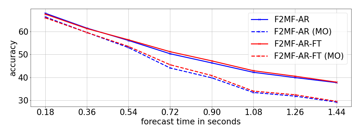
Figure 8: Dependence of the semantic segmentation accuracy of our autoregressive models on different forecasting offsets on Frankfurt videos from Cityscapes val. FT denotes autoregressive fine-tuning.

IV-G Cross-dataset generalization

We investigate whether our feature-based forecasting generalizes to unseen data beyond the validation subset, as proposed in [11]. We aim to test our models on the CamVid dataset [53] which differs from Cityscapes in terms of image resolution, video framerate and the set of semantic labels. No adaptation is needed regarding the image resolution because our model is fully convolutional. We sample CamVid videos each five timesteps, which is approximately equal to three timesteps in Cityscapes. We evaluate the mIoU accuracy according to a mapping from 19 Cityscapes classes to 11 CamVid classes.

Table VII shows the accuracy of our single-step and autoregressive models, and also the autoregressive approach from [11]. The columns show the oracle accuracy (mIoU), the forecast accuracy (mIoU) as well as the relative performance drop w.r.t. to the oracle model. We observe that our approach achieves the highest accuracy and also the lowest relative performance drop.

TABLE VII: Semantic segmentation forecasting on CamVid dataset with models trained on Cityscapes.

	Oracle	Forecast	Rel. perf.	Drop
Luc ar. ft. [11]	55.4	46.8	84.5%	-15.5%
F2MF-DN121	62.8	51.3	81.7%	-18.3%
F2MF-DN121 ar.	62.8	53.4	85.0%	-15.0%
F2MF-DN121 ar. ft.	62.8	54.5	86.8%	-13.2%

Figure 9 shows the performance of our best model from Table VII on two CamVid scenes. The rows show the last raw frame, ground truth and the forecasted segmentation. We observe that the feature forecasting succeeds to overcome the domain shift to a considerable degree.

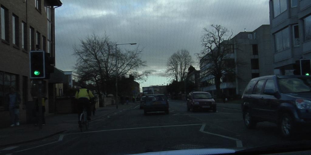
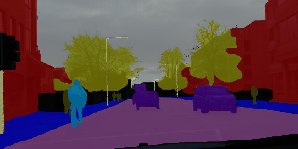
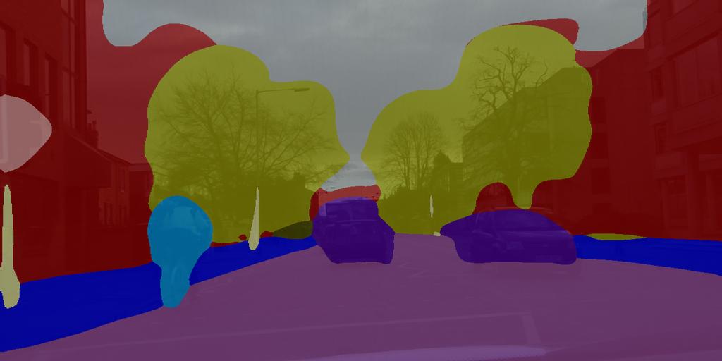
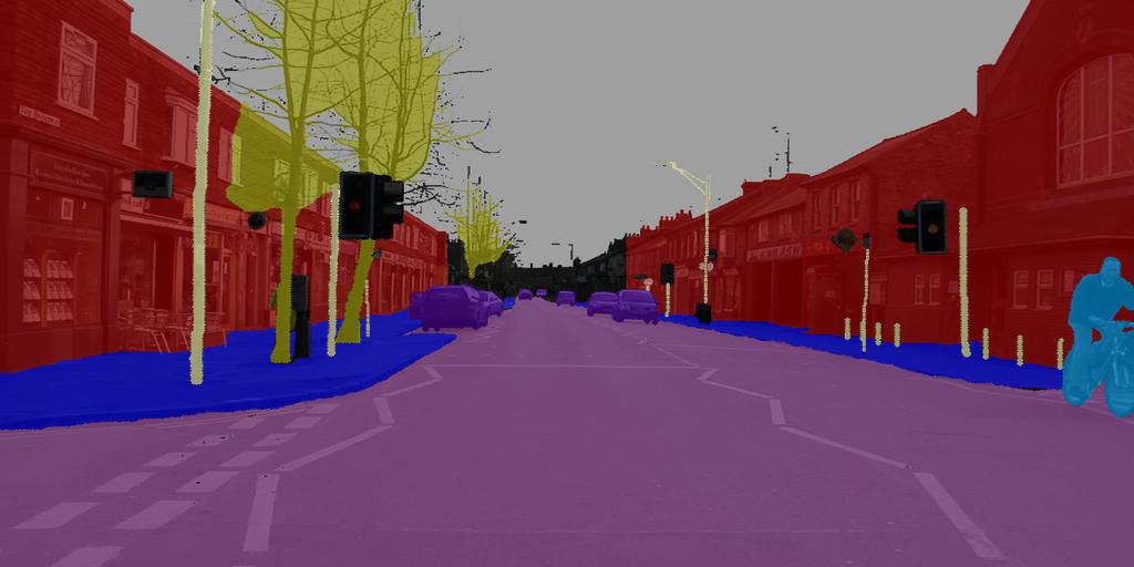
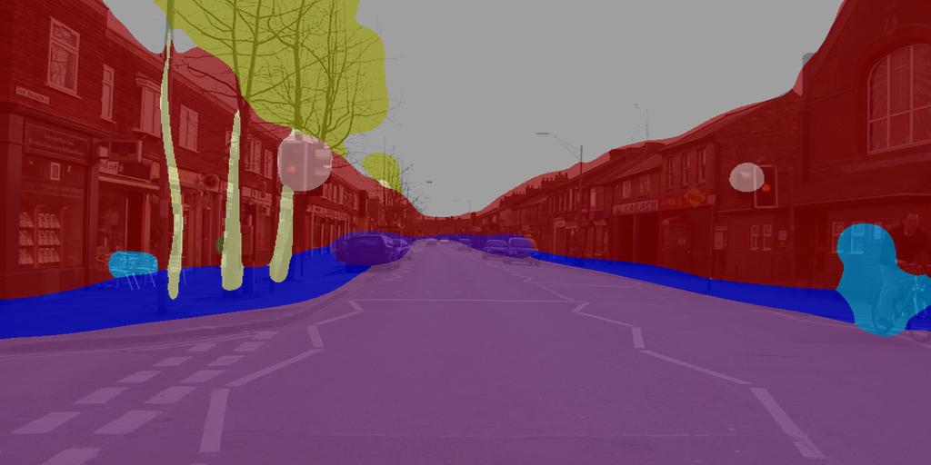
Figure 9: Mid-term forecast on two scenes from the CamVid dataset as produced by our best model from Table VII. The columns show the last observed frame, future ground truth and our F2MF forecast.

IV-H Interpreting the model decisions

Figure 10: Interpretation of F2F (rows 1,3) and F2MF (rows 2,4) decisions in two pixels denoted with green squares. We consider a pixel on the bicycle (rows 1-2) and a pixel on disoccluded background (rows 3-4). The columns show the four input frames, the forecasted semantic map, and the groundtruth with the overlayed future frame. Yellow squares show the positions of the considered two pixels in the observed frames. Red dots show top gradients of the green pixel max-log-softmax w.r.t. input. These dots correspond to input pixels which are most responsible for the model decision in the green pixel. We observe that the F2MF forecast establishes a better spatio-temporal focus than the F2M forecast.

This subsection further investigates the difference between F2MF and F2F forecasting for semantic segmentation. Figure 10 considers two particular output pixels and visualizes pixels with top 1‰ gradients of log-max-softmax w.r.t. to the input frames (red dots). Columns 1-4 show the four input frames. Columns 5-6 show our forecast and the ground truth. Pairs of rows correspond to two output pixels which are designated with a green square in the predictions and with a yellow square in the observed frames. Rows 1-2 consider a pixel located at the rear bicycle wheel in the future frame. We observe that most of the gradients are located at the corresponding spot in the most recent frame for both models. However, the gradients of the F2MF model are less spread and more focused towards the corresponding input pixel. Rows 3-4 consider a pixel which is occluded by the passing bicyclist in the most recent frame, while being disoccluded in the future frame. We observe that the F2F model relies on the context by looking around the pixel location in the most recent frame. On the other hand, the F2MF model realizes that this part of the scene had been visible in the most distant frame. Thus, our F2MF module makes the forecast just by copying the representation from the most distant feature tensor. This shows that our F2MF model is able to learn to handle complex occlusion patterns.

IV-I Computational Complexity

We analyze computational complexity of our methods and compare it with the corresponding state-of-the-art. We assume that the system is able to cache the necessary past activations and therefore consider the computational effort which is required to make the forecast after acquiring the current RGB frame. We report the count of multiply-accumulate operations (MAC) as measured with thop [54].

TABLE VIII: Computational complexity of semantic segmentation forecasting (GMAC) on full-resolution Cityscapes images.

Modules	M2M [14]	F2MF-DN121
Single-frame semantics	536.4	145.5
Flow (FlowNet2-C)	88.9	0.0
Forecasting	38.8	9.8
Total forecasting	127.7	9.8
Total	664.1	155.3

Table VIII compares our F2MF-based semantic segmentation forecasting with the runner-up method [14] from Table I. We observe that our forecasting incurs $12\times$ less complexity. The advantage remains considerable ($4\times$) even if we consider a comparison with single-frame semantics included. The difference mostly stems from the fact that our forecasting model operates on 1/32 resolution and does not require high resolution optical flow. The approach [14] has to evaluate PSP-Net and FlowNet2-C at 0.5 MPx, as well as to forecast flow features on 1/8 resolution. Our estimate assumes that their forecast requires evaluation of a single ConvLSTM cell with 74 feature maps both in the hidden state and the input [14].

Table IX compares our F2MF-based instance-level forecasting with the multi-level F2F approach [12]. The table shows the cost of single-frame inference and the cost of forecasting at each subsampling level. Our single-frame inference is a bit inefficient and requires around $1.6\times$ more compute than FPN based Mask R-CNN. Nevertheless, our total forecasting cost is $18\times$ smaller than multi-level F2F [12]. This is because we only forecast features which are $16\times$ subsampled w.r.t. to the input resolution. On the other hand, multi-level approaches [12, 15] additionally have to forecast expensive fine-resolution features at 1/8$\times$ and 1/4$\times$ resolution. We expect that [15] would suffer from the same problem although their source code is not available.

TABLE IX: Computational complexity of instance segmentation forecasting (GMAC).

Modules	F2F-M-FPN-RN50 [12]	F2MF-M-C4-RN50
Single-frame sem.	401.0	668.4
Forecasting at 1/4$\times$	1417.7	0.0
Forecasting at 1/8$\times$	354.4	0.0
Forecasting at 1/16$\times$	88.6	106.2
Forecasting at 1/32$\times$	22.1	0.0
Total Forecasting	1865.2	106.2
Total	2266.2	774.6

Table X shows unoptimized execution profiles of our forecasting models on a GTX1080Ti GPU. We measure the average time for three inference stages: feature extraction in four input frames, feature forecasting, and semantic formation. Sections correspond to three dense prediction tasks: semantic segmentation (top), instance segmentation (middle), and panoptic segmentation (bottom). We observe that forecasting is much faster than feature extraction and single-frame inference. F2MF-RN18 allows real-time inference since online execution environments allow to cache the past features and to perform feature extraction in only one frame — the most recent one.

TABLE X: Execution profile of unoptimized F2MF models (milliseconds).

Model	4$\times$ Extraction	Forecasting	Semantics
F2MF-RN18	72	7	7
F2MF-DN121	265	12	8
F2MF-Mask-C4-RN50	204	47	248
F2MF-PDL-RN50	230	52	144

V Conclusion

Anticipation of future semantics is a prerequisite for intelligent planning of current actions. Recent work addresses this problem by implicitly capturing laws of scene dynamics throughout deep learning in video. However, the existing approaches are unable to distinguish disoccluded and emerging scenery from previously observed parts of the scene. This is suboptimal, since the former requires pure recognition while the latter can be explained by warping. Different than all previous approaches, our method predicts emergence of unobserved scenery and exploits that information for disentangling variation caused by novelty from variation due to motion.

Our method performs dense semantic forecasting on the feature level. Different than previous such approaches, we regularize the forecasting process by expressing it as a causal relationship between the past and the future. The proposed F2M (feature-to-motion) forecasting generalizes better than the classic F2F (feature-to-feature) approach at many (but not all) image locations. We achieve the best of both worlds by blending F2M and F2F predictions with densely regressed weight factors. We empirically confirm that low F2M weights occur at unobserved scenery. The resulting F2MF approach surpasses the state-of-the-art in semantic segmentation forecasting on the Cityscapes dataset by a wide margin.

We complement convolutional features with their respective correlation coefficients organized within a cost volume over a small set of discrete displacements. Our forecasting models use deformable convolutions in order to account for geometric nature of F2F forecasting. These two improvements bring clear advantage in all three feature-level approaches: F2F, F2M, and F2MF. To the best of our knowledge, this is the first account of using these improvements for semantic forecasting.

Unlike previous methods, our single-frame model for semantic segmentation does not use skip connections along the upsampling path. Consequently, we are able to forecast condensed abstract features at the far end of the downsampling path with a single F2MF module. This greatly improves the inference speed and favors the forecasting accuracy due to coarse resolution and high semantic content of the involved features. We were unable to outperform this approach with multi-level F2F forecasting in spite of significantly better single-frame accuracy.

We also propose an adaptation of the proposed F2MF method for two additional dense prediction tasks: instance segmentation and panoptic segmentation. These experiments use third-party single-frame models and therefore show that our method can be successfully used as a drop-in solution for converting any kind of dense prediction model into its competitive forecasting counterpart. To the best of our knowledge, this is the first account of panoptic forecasting in the scientific literature.

The proposed method offers many exciting directions for future work. In particular, our method does not address multi-modal future, which is a key to long-term forecasting and worst-case reasoning. Other suitable extensions include overcoming obstacles towards end-to-end training, extension to RGB forecasting, as well as enforcing temporally consistent predictions in neighbouring video frames.

Josip Šarić received the M.Sc. degree in computer science from the University of Zagreb, Croatia. He is currently a Research Assistant at the Faculty of Electrical Engineering and Computing, University of Zagreb. His research interests include efficient convolutional architectures for image recognition and dense semantic forecasting.

Sacha Vražić is the Director of Autonomous Driving R&D at Rimac Automobili, where he works on solving issues to achieve the full autonomy for self-driving vehicles. He was heading the research laboratory for a Toyota Group company, and before he was teaching at University in Nice, France. He authored number of publications and patents. His research interest are in computer vision, machine learning and blind source separation.

Siniša Šegvić received the Ph.D. degree in computer science from the University of Zagreb, Croatia. He was a Post-Doctoral Researcher at IRISA Rennes, for one year, and as a Post-Doctoral Researcher at TU Graz, for one year. He is currently a Full Professor at the Faculty of Electrical Engineering and Computing, University of Zagreb. His research interests include efficient convolutional architectures for classification, dense prediction, and dense semantic forecasting.

References

- [1] K. He, G. Gkioxari, P. Dollár, and R. Girshick, “Mask r-cnn,” in Proc. ICCV, 2017, pp. 2961–2969.
- [2] B. Cheng, M. D. Collins, Y. Zhu, T. Liu, T. S. Huang, H. Adam, and L.-C. Chen, “Panoptic-deeplab: A simple, strong, and fast baseline for bottom-up panoptic segmentation,” in Proc. CVPR, June 2020.
- [3] A. J. Davison, I. D. Reid, N. Molton, and O. Stasse, “Monoslam: Real-time single camera SLAM,” IEEE Trans. Pattern Anal. Mach. Intell., vol. 29, no. 6, pp. 1052–1067, 2007.
- [4] Z. Zhang, “Camera calibration: a personal retrospective,” Mach. Vis. Appl., vol. 27, no. 7, pp. 963–965, 2016.
- [5] I. Krešo and S. Šegvic, “Improving the egomotion estimation by correcting the calibration bias,” in VISAPP (3), 2015, pp. 347–356.
- [6] S. Reuter, B. Vo, B. Vo, and K. Dietmayer, “The labeled multi-bernoulli filter,” IEEE Trans. Signal Proc., vol. 62, no. 12, pp. 3246–3260, 2014.
- [7] S. Oprea, P. Martinez-Gonzalez, A. Garcia-Garcia, J. A. Castro-Vargas, S. Orts-Escolano, J. Garcia-Rodriguez, and A. Argyros, “A review on deep learning techniques for video prediction,” IEEE Trans. Pattern Anal. Mach. Intell., 2020.
- [8] M. Mathieu, C. Couprie, and Y. LeCun, “Deep multi-scale video prediction beyond mean square error,” in ICLR, 2016.
- [9] H. Gao, H. Xu, Q.-Z. Cai, R. Wang, F. Yu, and T. Darrell, “Disentangling propagation and generation for video prediction,” in Proc. ICCV, 2019, pp. 9006–9015.
- [10] A. Alahi, K. Goel, V. Ramanathan, A. Robicquet, L. Fei-Fei, and S. Savarese, “Social lstm: Human trajectory prediction in crowded spaces,” in Proc. CVPR, 2016, pp. 961–971.
- [11] P. Luc, N. Neverova, C. Couprie, J. Verbeek, and Y. LeCun, “Predicting deeper into the future of semantic segmentation,” in Proc. ICCV, 2017, pp. 648–657.
- [12] P. Luc, C. Couprie, Y. Lecun, and J. Verbeek, “Predicting future instance segmentation by forecasting convolutional features,” in Proc. ECCV, 2018, pp. 584–599.
- [13] Y. Yao, M. Xu, C. Choi, D. J. Crandall, E. M. Atkins, and B. Dariush, “Egocentric vision-based future vehicle localization for intelligent driving assistance systems,” in ICRA, 2019.
- [14] A. Terwilliger, G. Brazil, and X. Liu, “Recurrent flow-guided semantic forecasting,” in Proc. WACV. IEEE, 2019, pp. 1703–1712.
- [15] J. Sun, J. Xie, J.-F. Hu, Z. Lin, J. Lai, W. Zeng, and W.-s. Zheng, “Predicting future instance segmentation with contextual pyramid convlstms,” in Proc. of the 27th ACM ICM, 2019, pp. 2043–2051.
- [16] J. Šarić, M. Oršić, T. Antunović, S. Vražić, and S. Šegvić, “Single level feature-to-feature forecasting with deformable convolutions,” in Proc. GCPR. Springer, 2019, pp. 189–202.
- [17] J. Šarić, M. Oršić, T. Antunović, S. Vražić, and S. Šegvić, “Warp to the future: Joint forecasting of features and feature motion,” in Proc. CVPR, June 2020.
- [18] B. Zhou, H. Zhao, X. Puig, T. Xiao, S. Fidler, A. Barriuso, and A. Torralba, “Semantic understanding of scenes through the ade20k dataset,” IJCV, vol. 127, no. 3, pp. 302–321, 2019.
- [19] P. Liu, M. R. Lyu, I. King, and J. Xu, “Selflow: Self-supervised learning of optical flow,” in Proc. CVPR, 2019, pp. 4571–4580.
- [20] R. Szeliski, Computer vision: algorithms and applications. Springer Science & Business Media, 2010.
- [21] A. Dosovitskiy, P. Fischer, E. Ilg, P. Hausser, C. Hazirbas, V. Golkov, P. Van Der Smagt, D. Cremers, and T. Brox, “Flownet: Learning optical flow with convolutional networks,” in Proc. ICCV, 2015, pp. 2758–2766.
- [22] D. Sun, X. Yang, M.-Y. Liu, and J. Kautz, “Pwc-net: Cnns for optical flow using pyramid, warping, and cost volume,” in Proc. CVPR, 2018, pp. 8934–8943.
- [23] J. Zbontar, Y. LeCun et al., “Stereo matching by training a convolutional neural network to compare image patches.” J. Mach. Learn. Res., vol. 17, no. 1, pp. 2287–2318, 2016.
- [24] V. Vukotić, S.-L. Pintea, C. Raymond, G. Gravier, and J. C. van Gemert, “One-step time-dependent future video frame prediction with a convolutional encoder-decoder neural network,” in Proc. ICIAP. Springer, 2017, pp. 140–151.
- [25] F. A. Reda, G. Liu, K. J. Shih, R. Kirby, J. Barker, D. Tarjan, A. Tao, and B. Catanzaro, “Sdc-net: Video prediction using spatially-displaced convolution,” in Proc. ECCV, 2018, pp. 718–733.
- [26] Y. Li, C. Fang, J. Yang, Z. Wang, X. Lu, and M.-H. Yang, “Flow-grounded spatial-temporal video prediction from still images,” in Proc. ECCV, 2018, pp. 600–615.
- [27] J. Pan, C. Wang, X. Jia, J. Shao, L. Sheng, J. Yan, and X. Wang, “Video generation from single semantic label map,” in Proc. CVPR, 2019, pp. 3733–3742.
- [28] Z. Hao, X. Huang, and S. Belongie, “Controllable video generation with sparse trajectories,” in Proc. CVPR, 2018, pp. 7854–7863.
- [29] T.-Y. Lin, P. Dollár, R. Girshick, K. He, B. Hariharan, and S. Belongie, “Feature pyramid networks for object detection,” in Proc. CVPR, 2017, pp. 2117–2125.
- [30] I. Kreso, J. Krapac, and S. Segvic, “Ladder-style densenets for semantic segmentation of large natural images,” in ICCV CVRSUAD, 2017, pp. 238–245.
- [31] I. Krešo, J. Krapac, and S. Šegvić, “Efficient ladder-style densenets for semantic segmentation of large images,” IEEE Trans. on ITS, 2020.
- [32] A. Bhattacharyya, M. Fritz, and B. Schiele, “Bayesian prediction of future street scenes using synthetic likelihoods,” in ICLR, 2019.
- [33] S. S. Nabavi, M. Rochan, and Y. Wang, “Future semantic segmentation with convolutional lstm,” BMVC, 2018.
- [34] X. Chen and Y. Han, “Multi-timescale context encoding for scene parsing prediction,” in 2019 IEEE ICME. IEEE, 2019, pp. 1624–1629.
- [35] C. Graber, G. Tsai, M. Firman, G. Brostow, and A. G. Schwing, “Panoptic segmentation forecasting,” in Proc. CVPR, 2021, pp. 12 517–12 526.
- [36] X. Jin, H. Xiao, X. Shen, J. Yang, Z. Lin, Y. Chen, Z. Jie, J. Feng, and S. Yan, “Predicting scene parsing and motion dynamics in the future,” in NIPS, 2017, pp. 6915–6924.
- [37] C. Feichtenhofer, A. Pinz, and A. Zisserman, “Convolutional two-stream network fusion for video action recognition,” in Proc. CVPR, 2016, pp. 1933–1941.
- [38] C. Vondrick, H. Pirsiavash, and A. Torralba, “Anticipating the future by watching unlabeled video,” arXiv:1504.08023, vol. 2, 2015.
- [39] J.-F. Hu, J. Sun, Z. Lin, J.-H. Lai, W. Zeng, and W.-S. Zheng, “Apanet: Auto-path aggregation for future instance segmentation prediction,” IEEE Trans. Pattern Anal. Mach. Intell., 2021.
- [40] C. Couprie, P. Luc, and J. Verbeek, “Joint Future Semantic and Instance Segmentation Prediction,” in ECCV W. on Antic. Human Beh., 2018, pp. 154–168.
- [41] H.-k. Chiu, E. Adeli, and J. C. Niebles, “Segmenting the future,” IEEE Robotics and Automation Letters, vol. 5, no. 3, pp. 4202–4209, 2020.
- [42] Z. Lin, J. Sun, J.-F. Hu, Q. Yu, J.-H. Lai, and W.-S. Zheng, “Predictive feature learning for future segmentation prediction,” in Proc. ICCV, 2021, pp. 7365–7374.
- [43] S. Vora, R. Mahjourian, S. Pirk, and A. Angelova, “Future semantic segmentation using 3d structure,” in ECCV 3D Recons. meets Seman. Work., 2018.
- [44] Y. Zhu, K. Sapra, F. A. Reda, K. J. Shih, S. D. Newsam, A. Tao, and B. Catanzaro, “Improving semantic segmentation via video propagation and label relaxation,” in CVPR, 2019, pp. 8856–8865.
- [45] A. Robinson, F. J. Lawin, M. Danelljan, F. S. Khan, and M. Felsberg, “Learning fast and robust target models for video object segmentation,” in CVPR, 2020, pp. 7404–7413.
- [46] D. Zhang, J. Han, L. Yang, and D. Xu, “SPFTN: A joint learning framework for localizing and segmenting objects in weakly labeled videos,” IEEE Trans. Pattern Anal. Mach. Intell., vol. 42, no. 2, pp. 475–489, 2020.
- [47] J. Han, L. Yang, D. Zhang, X. Chang, and X. Liang, “Reinforcement cutting-agent learning for video object segmentation,” in CVPR, 2018, pp. 9080–9089.
- [48] X. Zhu, H. Hu, S. Lin, and J. Dai, “Deformable convnets v2: More deformable, better results,” arXiv preprint arXiv:1811.11168, 2018.
- [49] M. Cordts, M. Omran, S. Ramos, T. Rehfeld, M. Enzweiler, R. Benenson, U. Franke, S. Roth, and B. Schiele, “The cityscapes dataset for semantic urban scene understanding,” in Proc. CVPR, 2016, pp. 3213–3223.
- [50] D. P. Kingma and J. Ba, “Adam: A method for stochastic optimization,” arXiv preprint arXiv:1412.6980, 2014.
- [51] M. Orsic, I. Kreso, P. Bevandic, and S. Segvic, “In defense of pre-trained imagenet architectures for real-time semantic segmentation of road-driving images,” in Proc. CVPR, 2019, pp. 12 607–12 616.
- [52] Y. Wu, A. Kirillov, F. Massa, W.-Y. Lo, and R. Girshick, “Detectron2,” https://github.com/facebookresearch/detectron2, 2019.
- [53] G. J. Brostow, J. Fauqueur, and R. Cipolla, “Semantic object classes in video: A high-definition ground truth database,” Pattern Recognition Letters, vol. 30, no. 2, pp. 88–97, 2009.
- [54] L. Zhu, “Thop: Pytorch-opcounter,” https://github.com/Lyken17/pytorch-OpCounter, 2020.