Lightweight Multi-Branch Network for Person Re-Identification

Abstract

Person Re-Identification aims to retrieve person identities from images captured by multiple cameras or the same cameras in different time instances and locations. Because of its importance in many vision applications from surveillance to human-machine interaction, person re-identification methods need to be reliable and fast. While more and more deep architectures are proposed for increasing performance, those methods also increase overall model complexity. This paper proposes a lightweight network that combines global, part-based, and channel features in a unified multi-branch architecture that builds on the resource-efficient OSNet backbone. Using a well-founded combination of training techniques and design choices, our final model achieves state-of-the-art results on CUHK03 labeled, CUHK03 detected, and Market-1501 with 85.1% mAP / 87.2% rank1, 82.4% mAP / 84.9% rank1, and 91.5% mAP / 96.3% rank1, respectively.

Index Terms—  Person Re-Identification, Deep Learning, Image Processing

1 Introduction

Person Re-Identification (PREID) is an important computer vision task for video surveillance applications. Formally, the problem can be stated as follows [1]. Given a probe image $\mathbf{P}$, and a gallery of $M$ images $\mathcal{G}=\{\mathbf{G}_{i}\}_{i=1}^{M}$, all of which annotated with an associated identity $\mathrm{id}(\mathbf{G}_{i})\in\mathbb{N}$, the goal is to find a similarity measure $\mathrm{sim}\left(\cdot\right)$ such that

$$i^{*}=\operatorname*{arg\,max}_{i=1,\dots,M}\mathrm{sim}(\mathbf{P},\mathbf{G}_{i}) \Rightarrow \mathrm{id}(\mathbf{P})=\mathrm{id}(\mathbf{G}_{i^{*}}).$$ (1)

While it is no surprise that the success of deep learning and the need for PREID as a processing step for person tracking has resulted in numerous approaches, the problem remains challenging, especially when it comes to balancing performance and low complexity of the models.

Recently, multiple-branch architectures have been proposed in particular [2, 3, 4, 5, 6]. These methods allow the network to focus on different person features in individual branches, e.g., on distinct spatial parts or channels. Although branching generally increases model performance, it comes with higher computational costs, especially if the number of branches or the total number of operations in them is increased. We claim that additional model complexity is not necessary and propose a network that outperforms other multi-branch approaches by using a suitable feature extractor and the right combination of training techniques.

The resulting network consists of three branches that optimize the global, partial, and channel-wise representations using simple computations, respectively. Despite this branching, we succeed in keeping the number of parameters low using OSNet [7], a lightweight feature extractor that has recently proven to be more efficient and accurate than other backbones for PREID tasks. Our deep neural network achieves state-of-the-art results on two important benchmark datasets, Market-1501 [8] and CUHK03 [9]. In detailed ablation studies, we demonstrate how the respective branches increase model performance, why our network performs better than other multi-branch approaches, and what training techniques are necessary to train a multi-branch architecture with OSNet backbone. Code and pretrained models of our research are publicly available.

2 Related Work

While PREID has been studied as a computer vision task for a long time [10], deep learning accelerated the research progress and model performance significantly, dominating the scene ever since [1, 11, 12, 7, 13, 2]. PREID approaches can be categorized as follows. First, several methods focus on improving feature extraction for the global input images [12, 7, 14]. Luo et al. [12] contributed with comprehensive research of many training techniques and were able to find combinations that boost the overall performance. Zhou et al. [7], on the other hand, concentrated on the feature extraction itself, proposing OSNet, a multi-scale network designed explicitly for the PREID task that outperforms standard ResNet50 [15] backbones despite a much lower number of parameters.

Another important research direction is finding spatial partitions of the persons’ images [13, 16, 3]. Usually, the input image is divided into disjoint parts, often horizontal stripes, to obtain partitioned features that are discriminative for person matching. Sun et al. [13] utilized the idea of part pooling, where the partitioning is done via spatial pooling after the convolutional layers of the backbone. This idea has since been used in other architectures [2, 3, 16]. In this context, many multi-branch or multi-stage approaches have been developed [2, 3, 6]. They mostly try to learn global and spatial part features in individual branches or combine part, channel, and global features, either through pooling [2, 3, 16] or attention [4, 5, 17, 18].

3 Methodology

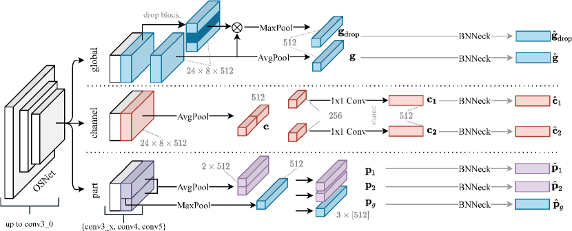
Fig. 1: Structure of our network. After forwarding images through the first three blocks of an OSNet backbone, our network continues in three distinct branches to learn global, channel-based and part-based features. All volumes are forwarded to BNNeck layers to produce final embeddings suited for different loss functions.

3.1 Network Architecture

Like all recent works on the problem, we design an end-to-end neural network architecture based on strong image feature extraction backbones pretrained on ImageNet [19]. In this subsection, we describe the architecture and training of the proposed network to solve Eq. (1). Our goal is to utilize a multi-branch architecture similar to MGN [2] and SCR [3] that leverages global, part-based and channel-based features, while keeping the overall number of parameters and embeddings low. Consequently and as illustrated in Fig. 1, our network consists of three branches: The global branch, the part branch, and the channel branch.

Let $\mathbf{X}\in\mathbb{R}^{384\times 128\times 3}$ be an input image. Before separating into distinct branches, the image $\mathbf{X}$ is passed through a truncated OSNet [7] backbone, up until the first layer of the third block, i.e., conv3_0, as in [6]. This concept has been employed before with ResNet50 [2, 3], using the first blocks up to conv4_0. We chose OSNet over ResNet due to its superior performance and lower complexity for PREID tasks [7, 6]. After forwarding $\mathbf{X}$ through the initial layers, the network forms the three branches, which comprise the remaining layers of OSNet up to the fifth block. By this design, only the layers up to conv3_0 are shared by all the branches, and for each individual branch, we obtain a tensor of dimension $24\times 8\times 512$.

In the global branch, we obtain two global representations as follows: First, we aggregate the information by applying 2D average pooling on the tensor, obtaining the $512$-dimensional vector $\mathbf{g}$. For the second global representation, the initial $24\times 8\times 512$-tensor is used as an input for a drop block, inspired by [20]. The drop block removes the highest activated horizontal regions from the tensor, forcing the network to emphasize on less discriminative regions, which increases the robustness of the resulting representation. Having removed the regions of highest activity, we apply 2D max pooling on the resulting tensor, obtaining another $512$-dimensional vector $\mathbf{g}_{\text{drop}}$.

In the channel branch, the initial $24\times 8\times 512$-tensor is reduced to a $512$-dimensional vector and then partitioned into two vectors of length $256$ each. We use $1\times 1$ convolutions to scale the representations back up, obtaining two $512$-dimensional vectors $\mathbf{c}_{1}$ and $\mathbf{c}_{2}$. Here, the parameters of the $1\times 1$ convolutions are shared among both channel parts.

Finally, in the part branch, we transform the initial $24\times 8\times 512$-tensor into three representations. We use average pooling to obtain a volume of size $2\times 1\times 512$ that we split into two $512$-dimensional part-based representations $\mathbf{p}_{1}$ and $\mathbf{p}_{2}$, representing the upper and lower body, respectively. Additionally, we use max pooling on the initial volume, obtaining another $512$-dimensional global representation $\mathbf{p}_{g}$ within the part branch.

We use a BNNeck [12] for all branch vector representations calculated in this way. Each BNNeck block consists of batch normalization and a fully connected to number-of-classes layer. The aim of this block is to optimize embeddings for two different metric spaces at the same time. Embeddings obtained before the batch normalization layer are used for optimization with respect to a ranking loss (e.g., triplet loss [21]), while embeddings obtained after the fully connected layer are used for optimization with respect to an identity loss (e.g., Cross-Entropy (CE) loss). Embeddings obtained after the batch normalization but before the fully connected layer find a balance between the representations of the two different metric spaces (i.e., ranking space and identitiy space) and are therefore used for inference. From the resulting embeddings we form two sets, given by

$$\mathcal{I} :=\left\{\hat{\mathbf{g}},\hat{\mathbf{g}}_{\text{drop}},\hat{\mathbf{p}}_{1},\hat{\mathbf{p}}_{2},\hat{\mathbf{p}}_{g},\hat{\mathbf{c}}_{1},\hat{\mathbf{c}}_{1}\right\},$$ (2)

$$\mathcal{R} :=\left\{\mathbf{g},\mathbf{g}_{\text{drop}},\mathbf{p}_{g}\right\},$$ (3)

for training in identity and rank spaces, respectively, where $\hat{\cdot}$ denotes the tensors of the BNNeck representations after the fully connected layer.

3.2 Training and Loss Functions

For training, we use a combination of CE loss and Multi-Similarity (MS) loss  [22]. The latter was designed to take advantage of existing pair-wise methods and sampling strategies by exploiting a soft weighting scheme that considers both self-similarity and relative similarity. We compute MS loss $\mathcal{L}_{\text{MS}}$ for global embeddings $\mathcal{R}$ obtained before batch normalization, and CE loss $\mathcal{L}_{\text{CE}}$ on all embeddings $\mathcal{I}$ obtained after applying softmax activation to the fully connected layer, i.e.,

$$\mathcal{L}_{\text{MS}}\left(f(\mathbf{X}),y)\right) :=\sum_{\mathbf{r}\in\mathcal{R}}\mathcal{L}_{\text{MS}}\left(\mathbf{r},y\right),$$ (4)

$$\mathcal{L}_{\text{CE}}\left(f(\mathbf{X}),y)\right) :=\sum_{\mathbf{i}\in\mathcal{I}}\mathcal{L}_{\text{CE}}\left(\mathbf{i},y\right),$$ (5)

where $f(\mathbf{X})$ is our networks output when forwarding $\mathbf{X}$. For CE loss $\mathcal{L}_{\text{CE}}$, we further use label smoothing [23, 12], which is a regularization technique that encourages the model not to be too confident on the training data. It adds a uniform noise distribution in CE calculation to soften the ground truth labels, which helps to improve model generalization. Thus, the overall objective loss function is

$$\mathcal{L}=\lambda_{\text{CE}}\mathcal{L}_{\text{CE}}+\lambda_{\text{MS}}\mathcal{L}_{\text{MS}},$$ (6)

where $\lambda_{\text{CE}}$ and $\lambda_{\text{MS}}$ are suitable weights. Additionally, we use random erasing augmentation (REA) [24], which randomly substitutes a rectangle with the image’s mean value. It has demonstrated to improve model generalization and to produce higher variance training data. Cosine annealing strategies are common in PREID networks [7, 25]. To further boost performance, we use warm-up cosine annealing [26, 27] as our learning rate strategy rather than traditional step learning rate schedules. The learning rate first grows linearly from $6\cdot 10^{-5}$ to $6\cdot 10^{-4}$ in 10 epochs, then cosine decay to $6\cdot 10^{-7}$ is applied in the remaining epochs. The learning rate $\operatorname{lr}(t)$ at epoch $t$ with $T$ total epochs is given by

$$\operatorname{lr}(t)=\left\{\begin{array}[]{ll}6\cdot 10^{-4}\cdot\frac{t}{10},&\text{ if }t\leq 10\\ 6\cdot 10^{-4}\cdot\frac{1}{2}\left(1+\cos\left(\pi\frac{t-10}{T-10}\right)\right),&\text{ if }10<t\leq T.\end{array}\right.$$

4 Experimental Results

Table 1: Comparison of our method with state-of-the-art. The table lists our results on the two most used benchmarks, Market-1501 and CHUK03. The latter was evaluated on the labeled set (CHUK03-L) and the detection set (CHUK03-D) in multi-gallery-shot setting (cf. [28]). Note that all results are reported without re-ranking (cf. [28]).

				Market-1501		CHUK03-L		CHUK03-D
Type	Method	Publication	Backbone	r1	mAP	r1	mAP	r1	mAP
Global feature	BagOfTricks [12]	CVPRW’19	ResNet50	94.5	85.9	–	–	–	–
	OSNet [7]	ICCV’19	OSNet	94.8	84.9	–	–	72.3	67.8
	BDB [14]	ICCV’19	ResNet50	95.3	86.7	79.4	76.7	76.4	73.5
Part-based	PCB+RPP [13]	ECCV’18	ResNet50	93.8	81.6	–	–	–	–
	MGN [2]	ACM MM 18	ResNet50	95.7	86.9	68.0	67.4	66.8	66.0
	Pyramid [16]	CVPR’19	ResNet101	95.7	88.2	78.9	76.9	79.9	74.8
	SCR [3]	WACV’20	ResNet50	95.7	89.0	83.8	80.4	82.2	77.6
Attention-based	MHN [4]	ICCV’19	ResNet50	95.1	85.0	77.2	72.4	71.7	65.4
	ABD [5]	ICCV’19	ResNet50	95.6	88.3	–	–	–	–
	PLR-OSNet [6]	PRCV ’20	OSNet	95.6	88.9	84.6	80.5	80.4	77.2
	SCSN [17]	CVPR’20	ResNet50	95.7	88.5	86.8	84.0	84.7	81.0
	Compact Re-ID [18]	ACM ICMR ’20	other	96.2	89.7	–	–	–	–
Ours	LightMBN		OSNet	96.3	91.5	87.2	85.1	84.9	82.4
	LightMBN (computed via [8])		OSNet	96.3	91.2	87.2	83.8	84.9	81.0

Datasets. We evaluated the model on two of the most widely used large-scale datasets, Market-1501 [8] and CUHK03 [9]. The Market-1501 dataset contains 32,668 images of 1,501 persons across 6 cameras, whereas the CUHK03 dataset comprises 13,164 images of 1,360 person across 6 cameras. For CUHK03, we use the new 767-split protocol [28], obtaining results for the labeled (CUHK03-L) and detected (CUHK03-D) configurations separately. We did not evaluate on DukeMTMC-ReID since use of this dataset has been prohibited by the authors.

Training Details. For training, input images are normalized to channel-wise zero-mean and a standard variation of 1 and spatial resolution of $384\times 128$. Data augmentation is performed by resizing images to 105% width and height and random cropping, as well as random horizontal flip with a probability of 0.5. Models are trained for 140 epochs for Market-1501 and 180 epochs for CUHK03 with a batchsize of 48. A batch consists of 8 samples for 6 identities each. The parameters are optimized by using using the Adam optimizer [29] with $\epsilon=1e-8$, $\beta_{1}=0.9$ and $\beta_{2}=0.999$. The backbones are pre-trained on ImageNet [19] and all experiments are implemented with PyTorch [30]. To balance the losses we chose $\lambda_{\text{CE}}=\lambda_{\text{MS}}=0.5$.

Evaluation Details. Cosine distance is utilized to compute cumulative matching characteristics (CMC) [31]. Query and gallery images are re-sized to $384\times 128$ pixels and normalized. For a fair comparison with other existing methods, the CMC rank-1 accuracy (r1) and mean Average Precision (mAP) are reported as evaluation metrics. Results with the same identity and the same camera ID as the query image are not counted. The authors of [32] state in their official code repository that mAP values computed with recent PREID frameworks are about 1%-point higher than those computed by the original Matlab evaluation code of Market-1501 [8]. We were able to reproduce this. For completeness and fair comparison, we also state the mAP values for our final models as computed by the original evaluation script. We hope to raise more awareness to this issue by providing both results.

Table 2: Ablation study of branch influences. We investigate our models performance under the specified branch configurations, where G+C+P refers to our original model.

	Market-1501		CUHK03-D
Branch	rank1	mAP	rank1	mAP
Global (G)	95.4	89.3	80.8	77.3
Channel (C)	95.9	88.8	74.7	71.2
Part (P)	95.9	90.2	80.3	77.9
C+P	96.1	91.2	82.7	79.8
G+C	96.0	90.9	82.0	79.7
G+P	96.1	91.2	83.4	81.3
G+C+P	96.3	91.5	84.9	82.4

4.1 Comparison with State-of-the-Arts

Table 1 compares the performance of our model with that of other recent methods. Our model achieves state-of-the-art results on Market-1501, CUHK-L and CUHK-D, both in terms of rank-1 accuracy and mAP. The large difference in performance with regard to the mAP on all datasets is particularly noticeable. Interestingly, despite its simplicity, our architecture achieves better performance than other multi-branch approaches. Architecturally, our model is closely related to previous work such as MGN [2], PLR-OSNet [6], and, in particular, SCR [3]. All of these approaches use a truncated backbone followed by branching. MGN relies on ResNet50 and only uses spatial partitions, whereas our model builds upon OSNet and also better exploits the PREID problem by additionally using channel partitions. In this regard, SCR is the most similar architecture since both spatial and channel partitions are used for multi-loss training. However, for good performance, SCR requires nearly twice as many embeddings as our model and creates part and channel partitions in the same branch, which could theoretically impede the branches’ specialization.

4.2 Ablation Study

Influence of Branches. When introducing branches to a neural network architecture, the parameter count can raise substantially. Thus, any such introduction has to be well-justified. Table 2 depicts our network’s performance for different branch combinations. The results suggest that single branches perform similarly when the other two respective branches are deactivated. Among all branches, the channel branch has the lowest performance on CUHK03-D, indicating that global features are very important for generalization on this dataset. As can be seen by the pairwise combination of branches, the part branch influences the performance significantly on CUHK03-D. By using all three branches together, our model achieves state-of-the-art results on both datasets.

Influence of Backbones. Table 3 shows some examples of the different performances of ResNet50 and OSNet. The raw model with ResNet50 (i.e., the one without beneficial additions) has the weakest performance among all models. Only with all possible additions it is able to achieve similar performance of a raw model with OSNet backbone. The best configuration that can be achieved with ResNet50 is still inferior than our final model. Our model with OSNet backbone only has about 9 million parameters, compared to about 23 million with ResNet50 backbone.

Influence of Learning Rate Schedule. As can be seen in Table 3, when substituting the cosine warmup annealing schedule with a constant schedule, performance decreases. For the constant schedule, we have reduced the initial learning rate of $6\times 10^{-4}$ three times by a factor of $10$ in the 50th, 80th and 110th epoch, respectively. The results indicate the importance of a suitable learning rate strategy for PRID on both datasets.

Influence of Drop Block. The results in Table 3 suggest that the drop block has hardly any influence on the performance on Market-1501. On the other hand, results on the CUHK03 dataset clearly show that the drop block can lead to better generalization on the test set and increases both metrics.

Table 3: Ablation study of training techniques. We investigate our models performance under the specified training modifications. Here, WCA indicates use of warmup cosine annealing, MS the use of MS loss over triplet loss, DB the use of drop block, and OSNet the use of OSNet over ResNet50 as backbone, respectively.

Configuration				Market-1501		CUHK03-D
OSNet	WCA	MS	DB	r1	mAP	r1	mAP
✗	✗	✗	✗	95.4	87.9	71.7	70.3
✗	✓	✓	✓	96.1	90.4	81.0	79.1
✓	✗	✗	✗	96.1	90.2	78.2	75.2
✓	✓	✗	✗	96.2	91.1	83.5	81.1
✓	✓	✗	✓	96.3	91.5	83.2	80.9
✓	✗	✓	✓	96.0	90.6	78.8	76.3
✓	✓	✓	✗	96.2	91.2	83.4	80.9
✓	✓	✓	✓	96.3	91.5	84.9	82.4

Influence of Loss Functions. We trained various modifications of our model with triplet loss instead of MS loss. Using MS loss in the final model slightly increases the rank-1 and mAP performance on CUHK03, but not on Market-1501. Thus, the choice of ranking loss function can be important for generalization on smaller datasets.

5 Conclusion

We have presented a multi-branch neural network that achieves state-of-the-art results on Market-1501 and CUHK03. Although branches increase the overall parameter count, we can keep the overall model complexity low by utilizing a lightweight OSNet backbone and suitable training techniques. The distinct branches of our network can capture the essential person features. Overall our research suggests that learning rate schedules and the backbone choice heavily influence the model performance and that drop blocks and MS loss assist the model in generalizing the smaller CUHK03 dataset. We conclude that multi-branch architectures should focus on the right combination of training techniques and OSNet feature extraction in favor of adding model complexity.

References

- [1] Liang Zheng, Yi Yang, and Alexander G Hauptmann, “Person re-identification: Past, present and future,” arXiv preprint arXiv:1610.02984, 2016.
- [2] Guanshuo Wang, Yufeng Yuan, Xiong Chen, Jiwei Li, and Xi Zhou, “Learning discriminative features with multiple granularities for person re-identification,” in Proceedings of the 26th ACM international conference on Multimedia, 2018, pp. 274–282.
- [3] Hao Chen, Benoit Lagadec, and Francois Bremond, “Learning discriminative and generalizable representations by spatial-channel partition for person re-identification,” in The IEEE Winter Conference on Applications of Computer Vision, 2020, pp. 2483–2492.
- [4] Binghui Chen, Weihong Deng, and Jiani Hu, “Mixed high-order attention network for person re-identification,” in Proceedings of the IEEE International Conference on Computer Vision, 2019, pp. 371–381.
- [5] Tianlong Chen, Shaojin Ding, Jingyi Xie, Ye Yuan, Wuyang Chen, Yang Yang, Zhou Ren, and Zhangyang Wang, “Abd-net: Attentive but diverse person re-identification,” in Proceedings of the IEEE International Conference on Computer Vision, 2019, pp. 8351–8361.
- [6] Ben Xie, Xiaofu Wu, Suofei Zhang, Shiliang Zhao, and Ming Li, “Learning diverse features with part-level resolution for person re-identification,” arXiv preprint arXiv:2001.07442, 2020.
- [7] Kaiyang Zhou, Yongxin Yang, Andrea Cavallaro, and Tao Xiang, “Omni-scale feature learning for person re-identification,” in Proceedings of the IEEE International Conference on Computer Vision, 2019, pp. 3702–3712.
- [8] Liang Zheng, Liyue Shen, Lu Tian, Shengjin Wang, Jingdong Wang, and Qi Tian, “Scalable person re-identification: A benchmark,” in Proceedings of the IEEE international conference on computer vision, 2015, pp. 1116–1124.
- [9] Wei Li, Rui Zhao, Tong Xiao, and Xiaogang Wang, “Deepreid: Deep filter pairing neural network for person re-identification,” in CVPR, 2014.
- [10] Niloofar Gheissari, Thomas B Sebastian, and Richard Hartley, “Person reidentification using spatiotemporal appearance,” in 2006 IEEE Computer Society Conference on Computer Vision and Pattern Recognition (CVPR’06). IEEE, 2006, vol. 2, pp. 1528–1535.
- [11] Mang Ye, Jianbing Shen, Gaojie Lin, Tao Xiang, Ling Shao, and Steven CH Hoi, “Deep learning for person re-identification: A survey and outlook,” arXiv preprint arXiv:2001.04193, 2020.
- [12] Hao Luo, Youzhi Gu, Xingyu Liao, Shenqi Lai, and Wei Jiang, “Bag of tricks and a strong baseline for deep person re-identification,” in Proceedings of the IEEE Conference on Computer Vision and Pattern Recognition Workshops, 2019, pp. 0–0.
- [13] Yifan Sun, Liang Zheng, Yi Yang, Qi Tian, and Shengjin Wang, “Beyond part models: Person retrieval with refined part pooling (and a strong convolutional baseline),” in Proceedings of the European Conference on Computer Vision (ECCV), 2018, pp. 480–496.
- [14] Zuozhuo Dai, Mingqiang Chen, Xiaodong Gu, Siyu Zhu, and Ping Tan, “Batch dropblock network for person re-identification and beyond,” in Proceedings of the IEEE International Conference on Computer Vision, 2019, pp. 3691–3701.
- [15] Kaiming He, Xiangyu Zhang, Shaoqing Ren, and Jian Sun, “Deep residual learning for image recognition,” in Proceedings of the IEEE conference on computer vision and pattern recognition, 2016, pp. 770–778.
- [16] Feng Zheng, Cheng Deng, Xing Sun, Xinyang Jiang, Xiaowei Guo, Zongqiao Yu, Feiyue Huang, and Rongrong Ji, “Pyramidal person re-identification via multi-loss dynamic training,” in Proceedings of the IEEE Conference on Computer Vision and Pattern Recognition, 2019, pp. 8514–8522.
- [17] Xuesong Chen, Canmiao Fu, Yong Zhao, Feng Zheng, Jingkuan Song, Rongrong Ji, and Yi Yang, “Salience-guided cascaded suppression network for person re-identification,” in Proceedings of the IEEE/CVF Conference on Computer Vision and Pattern Recognition, 2020, pp. 3300–3310.
- [18] Hussam Lawen, Avi Ben-Cohen, Matan Protter, Itamar Friedman, and Lihi Zelnik-Manor, “Compact network training for person reid,” in Proceedings of the 2020 International Conference on Multimedia Retrieval, 2020, pp. 164–171.
- [19] Alex Krizhevsky, Ilya Sutskever, and Geoffrey E Hinton, “Imagenet classification with deep convolutional neural networks,” in Advances in neural information processing systems, 2012, pp. 1097–1105.
- [20] Rodolfo Quispe and Helio Pedrini, “Top-db-net: Top dropblock for activation enhancement in person re-identification,” arXiv preprint arXiv:2010.05435, 2020.
- [21] Florian Schroff, Dmitry Kalenichenko, and James Philbin, “Facenet: A unified embedding for face recognition and clustering,” in Proceedings of the IEEE conference on computer vision and pattern recognition, 2015, pp. 815–823.
- [22] Xun Wang, Xintong Han, Weilin Huang, Dengke Dong, and Matthew R Scott, “Multi-similarity loss with general pair weighting for deep metric learning,” in Proceedings of the IEEE Conference on Computer Vision and Pattern Recognition, 2019, pp. 5022–5030.
- [23] Christian Szegedy, Vincent Vanhoucke, Sergey Ioffe, Jon Shlens, and Zbigniew Wojna, “Rethinking the inception architecture for computer vision,” in Proceedings of the IEEE conference on computer vision and pattern recognition, 2016, pp. 2818–2826.
- [24] Zhun Zhong, Liang Zheng, Guoliang Kang, Shaozi Li, and Yi Yang, “Random erasing data augmentation,” arXiv preprint arXiv:1708.04896, 2017.
- [25] Xiangyu Zhu, Zhenbo Luo, Pei Fu, and Xiang Ji, “Voc-reid: Vehicle re-identification based on vehicle-orientation-camera,” in Proceedings of the IEEE/CVF Conference on Computer Vision and Pattern Recognition Workshops, 2020, pp. 602–603.
- [26] Priya Goyal, Piotr Dollár, Ross Girshick, Pieter Noordhuis, Lukasz Wesolowski, Aapo Kyrola, Andrew Tulloch, Yangqing Jia, and Kaiming He, “Accurate, large minibatch sgd: Training imagenet in 1 hour,” arXiv preprint arXiv:1706.02677, 2017.
- [27] Tong He, Zhi Zhang, Hang Zhang, Zhongyue Zhang, Junyuan Xie, and Mu Li, “Bag of tricks for image classification with convolutional neural networks,” in Proceedings of the IEEE Conference on Computer Vision and Pattern Recognition, 2019, pp. 558–567.
- [28] Zhun Zhong, Liang Zheng, Donglin Cao, and Shaozi Li, “Re-ranking person re-identification with k-reciprocal encoding,” in Proceedings of the IEEE Conference on Computer Vision and Pattern Recognition, 2017, pp. 1318–1327.
- [29] Diederik P Kingma and Jimmy Ba, “Adam: A method for stochastic optimization,” arXiv preprint arXiv:1412.6980, 2014.
- [30] Adam Paszke, Sam Gross, Soumith Chintala, Gregory Chanan, Edward Yang, Zachary DeVito, Zeming Lin, Alban Desmaison, Luca Antiga, and Adam Lerer, “Automatic differentiation in pytorch,” 2017.
- [31] Hyeonjoon Moon and P Jonathon Phillips, “Computational and performance aspects of pca-based face-recognition algorithms,” Perception, vol. 30, no. 3, pp. 303–321, 2001.
- [32] Alexander Hermans, Lucas Beyer, and Bastian Leibe, “In defense of the triplet loss for person re-identification,” arXiv preprint arXiv:1703.07737, 2017.