On the Performance of Spectrum Sharing Backscatter Communication Systems

Abstract

Spectrum sharing backscatter communication systems are among the most prominent technologies for ultra-low power and spectrum efficient communications. In this paper, we propose an underlay spectrum sharing backscatter communication system, in which the secondary network is a backscatter communication system. We analyze the performance of the secondary network under a transmit power adaption strategy at the secondary transmitter, which guarantees that the interference caused by the secondary network to the primary receiver is below a predetermined threshold. We first derive a novel analytical expression for the cumulative distribution function (CDF) of the instantaneous signal-to-noise ratio of the secondary network. Capitalizing on the obtained CDF, we derive novel accurate approximate expressions for the ergodic capacity, effective capacity and average bit error rate. We further validate our theoretical analysis using extensive Monte Carlo simulations.

I Introduction

Legacy cellular networks have been designed with the ambition to provide voice services and high-speed data internet. Although, the race toward enhanced mobile broadband (eMBB) has continued for 5G and beyond networks, other use-cases have emerged, i.e., ultra reliable low latency communications (URLLC) and massive machine type communications (mMTC) [1, 2]. In mMTC, a massive number of low-cost devices is required to communicate with minimal power consumption. This paradigm opens the door for several Internet of Things (IoT) applications such as smart cities, homes, and agriculture with 21 billion expected devices by 2025 [3].

In this regard, several wireless technologies have recently emerged to achieve such low-power communications with low-cost devices. For example, low power long range wide area network (LoRaWAN) and SigFoX operate in unlicensed spectrum to provide low power wide area networks (LPWAN), while narrowband Internet of things (NB-IoT) technology makes use of licensed frequency bands to provide higher reliable communication [4, 5, 6]. The power consumption in these networks is considerably low, and the devices have long battery life and low cost. Hence, they are suitable for many IoT scenarios. Nevertheless, some applications require even ultra-low-power wireless communication and self-sustainable networks, which can not be achieved with the technologies adopted for LPWAN.

In this context, backscatter communications (BC) is one of the most prominent technologies for ultra-low-power communications. The tag (i.e., backscatter transmitter) modulates its information bits over the incident electromagnetic wave and reflects it to a receiver [7]. The interest in BC shines through its outstanding features, e.g., the transceivers in BC do not require power-hungry components such as oscillators, mixers, and amplifiers. Therefore, they have low-cost and complexity while requiring a small amount of power that can be easily harvested from the environment[8]. Also, BC is considered a green technology, where it usually does not require a battery. For these reasons, it is a potential candidate for self-sustainable wireless IoT networks.

The BC can be classified according to the adopted architecture into three categories: (i) monostatic backscatter, where a tag modulates a signal that is generated by a reader, then reflects it back to the reader; (ii) bistatic backscatter, where the tag backscatters the signal generated by a continuous wave (CW) source to the designated receiver; (iii) ambient backscatter, where the tag backscatters an incident signal from an ambient radio frequency (RF) source, rather than considering a dedicated source [9, 10].

Besides the low power requirement, another issue that faces wireless communications, in general, is spectrum scarcity. The enormous expansion of wireless communication systems with dedicated frequency bands (e.g., cellular networks, LPWAN, TV broadcast, and satellite communications) results in radio spectrum congestion [11]. This issue clearly appears in mMTC, where we may need to allocate spectrum bands to a tremendous number of devices. A possible solution to this problem is spectrum sharing, where multiple users can share the same frequency band under some conditions on the interference. One enabling technology for spectrum sharing is by adopting cognitive radios, where the transceivers are aware of the environment and can accordingly adapt their transmission characteristics, e.g., the power and frequency. In CR, a secondary network wisely shares the spectrum with a primary network that operates on licensed frequency [12, 13].

In this regard, spectrum sharing backscatter communications (SSBC), which exploits both CR and BC technologies, has been proposed as a potential solution for both the power limitation and spectrum scarcity issues in IoT networks. SSBC can be classified mainly into two modes according to the interference management mechanism, i.e., (i) overlay and (ii) underlay. In overlay networks, the secondary trasmitter (ST) harvests energy during the operation time of the primary trasmitter (PT). Then, it uses such energy to transmit when the PT is idle. Although SSBC systems operating in overlay mode are self-sustainable and interference-free networks, the affordable rate for secondary networks can be limited. This can be attributed to two reasons: (i) low harvested energy when the idle time of the PT is significantly high; (ii) insufficient possible transmission time when the PT frequently accesses the channel, i.e., low idle time. For underlay networks, the ST and PT can simultaneously access the channel. However, the ST should control its power to limit the interference at the primary receiver (PR) below a predefined threshold [14, 15]. In the following, we review the literature regarding BC and SSBC performance analysis.

I-1 Performance Analysis of BC

In [9], differential modulation is proposed to reduce the bit error rate (BER) and maximize the sum rate in ambient BC. The BER of the proposed scheme is derived to demonstrate the error performance of the system. In [16], a coding scheme is considered for ambient BC with tags that can have three states: no-backscatter, positive phase backscatter, and negative phase backscatter. The coding scheme maps each two consequence ternary symbols into three binary bits to increase the throughput. A higher-order modulation scheme is adopted to increase the uplink rate in [17], where a coded modulation scheme with forward error correction (FEC) is proposed to compensate for the power loss associated with higher-order modulation. In [18], a hybrid architecture that combines an ambient BC and a classical modulator with CW generator is presented. The modulation technique is selected to maximize the system performance, depending on the ambient environment. The throughput, energy outage, and coverage probability of the scheme are analyzed using stochastic geometry.

A non-coherent scheme for an ambient BC is designed in [19]. In this method, the transmitter considers differential modulation. The receiver adopts either a maximum likelihood (ML) detector or an energy detector that compares the power of the recent two consecutive symbols with optimal thresholds. Also, the BER and outage probability are derived in closed-form. In [20], a semi-coherent scheme that estimates some channel-related parameters is proposed. The error performance is analyzed for ambient sources that adopt either complex Gaussian wave or phase shift keying (PSK) modulation.

Since many communication systems consider orthogonal frequency-division multiplexing (OFDM), a BC scheme is proposed in [21], where the tag modulates the ambient OFDM wave at a rate much lower than that of the incident signal. Hence, the reflected wave can be seen as a spread spectrum signal. The optimal decoder is derived for both single and multi-antenna receivers. Then, the BER and data rate are investigated. In [22], the authors exploit the ambient OFDM signal to provide $M-$ary BC. The receiver considers a noncoherent energy detector, and the error performance is analytically investigated.

Regarding the capacity analysis, the ergodic capacity of ambient BC is derived in [23]. The capacity of the ambient source that considers OFDM is also analyzed under the interference from the BC. The authors in [24] compute the constrained capacity for binary phase shift keying (BPSK) and $M$-ary modulation by maximizing the mutual information between the reflected wave from the tag and received signal.

For monostatic BC with multi-tags, an energy-efficient scheme is proposed in [25], where the tags with the largest signal-to-noise ratio (SNR) are selected. The exact and asymptotic expressions for the ergodic and effective capacity are derived. Another tag selection scheme relying on time division multiple access (TDMA) is suggested [26].

I-2 Spectrum Shared BC

An RF-powered CR architecture is proposed in [27]. In this scheme, the ST can operate either in harvest-then-transmit mode or in a backscatter mode. The optimal duration of each operational mode is formulated as an optimization problem. On the other hand, the game theory is exploited for the mode selection in [28]. Another RF-powered CR system is proposed in [29], where the ST performs spectrum sensing first to select the operational mode. The energy efficiency of the secondary network is maximized by optimizing the duration of various modes, e.g., energy harvesting, BC, data transmission, and spectrum sensing phases.

In [30], a cooperative SSBC scheme is presented, where the PT simultaneously sends its own modulated symbols plus a carrier as a CW source for the secondary BC network. The optimal power allocation for the carrier and the optimal channel access time are computed to maximize the secondary system rate while preserving a minimum target rate for the primary network. Another cooperative RF-powered CR technique called symbiotic radio is visioned in [31]. In this scheme, the primary network and the secondary BC system are cooperative, as the primary network can benefit from the backscattered signal to enhance its channel. A possible realization of such a system is by considering the tag as a reconfigurable intelligent surface (RIS), i.e., a surface composed of many reflection elements with reconfigurable reflection coefficients [32, 33]. In this regard, the RIS phase profile and the beamforming are designed to minimize the transmission power while assuring a minimum Quality of Service (QoS) for both the primary and BC networks [34].

Most of the aforementioned schemes either consider the performance analysis of monostatic or mostly ambient BC. Each of these schemes has its own merits in terms of complexity, power efficiency, and reliability. In particular, monostatic backscatter can suffer from round-trip path loss as both the CW source and receiver are located on the same device, i.e., the reader. For ambient backscatter, it is the most prominent scheme from a power perspective. Nevertheless, the harvested energy and the system reliability depend on the availability of the ambient sources [21, 7]. On the other hand, bistatic backscatter can provide a compromise between reliability and power efficiency and a more flexible deployment of the network with separated CW source and receiver.

In this paper, we propose an underlay SSBC system in which the secondary network is a BC system consisting of a single ST operating as a CW source, a single tag (T) and a single secondary receiver (SR). The secondary network is operating in the presence of a primary network consisting of a transmitter-receiver pair. The performance of the proposed system is analyzed under a transmit power adaption strategy at the ST to ensure that the interference caused by the secondary network to the PR is below a predetermined threshold. The proposed scheme is reliable and both power and spectrum efficient, because it considers bistatic BC and spectrum sharing. Nevertheless, its performance has not been investigated in the existing literature to the best knowledge of the authors. It is worth pointing out that the cascaded fading channel nature of the secondary system and the transmit power adaption at the ST complicate the SNR statistics, which in turn leads to cumbersome performance analysis. Therefore, this paper aims to derive novel analytical expressions for the aforementioned performance metrics. In particular, we study the ergodic capacity, effective capacity, and average BER of the secondary system. The contribution of this paper can be summarized as follows:

• We first derive a novel analytical expression for the cumulative distribution function (CDF) of the instantaneous SNR of the secondary system.

• Making use of the obtained CDF, we derive novel and accurate approximate expressions for the ergodic and effective capacities of the secondary system.

• We obtain an accurate approximate expression for the average BER of the secondary system, which is general enough to cover a broad class of binary modulation formats suitable for BC.

• We get an approximation for the moment generating function (MGF), based on which, we derive the average symbol error rate (SER) of $M$-ary phase shift keying (${M}$-PSK) modulation.

• We derive insightful closed-form asymptotic expressions for the ergodic capacity, effective capacity and average BER for large values of the average channel power gain of the secondary network.

The remainder of this paper is structured as follows. The system model is presented in Section II. The performance of the proposed system is analyzed in Section III. Section IV includes the numerical results, and Section V concludes.

II System model

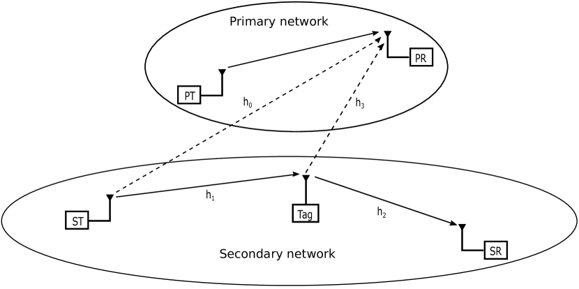
Figure 1: An underlay SSBC system in which a secondary BC network is sharing the spectrum of a primary network.

As shown in Fig. 1, we consider an underlay cognitive radio system in which a secondary network is allowed to share the spectrum of a primary network. The primary network consists of one PT and one PR. The secondary network is a BC system consisting of one ST that can be recognized as a CW source, one tag (T), and one SR. All terminals of the considered system are single antenna devices. The channel gains from the ST to PR and tag are, respectively, $h_{0}$ and $h_{1}$. The channel gains from the tag to SR and PR are $h_{2}$ and $h_{3}$, respectively. We assume that the aforementioned channel gains experience independent Rayleigh fading. Accordingly, the channel power gains $|h_{i}|^{2}$ for each $i\in\{0,1,2,3\}$ are exponentially distributed random variables (RVs). The CDF and probability density function (PDF) of $|h_{i}|^{2}$, denoted by $F_{|h_{i}|^{2}}(x)$ and $f_{|h_{i}|^{2}}(x)$, respectively, are given as

$$F_{|h_{i}|^{2}}(x)=(1-e^{-\frac{x}{\lambda_{i}}})\ u(x),$$ (1)

$$f_{|h_{i}|^{2}}(x)=\frac{1}{\lambda_{i}}e^{-\frac{x}{\lambda_{i}}}\ u(x),$$ (2)

where $i\in\{0,1,2,3\}$, $\lambda_{i}$ is the average (mean) of the RV $|h_{i}|^{2}$ and $u(x)$ is the unit step function. It should be noted that $\lambda_{i}$ is a positive real number that captures the propagation distance and the fading environment. We assume that the PT is distant from the SR and tag; hence, the interference caused by the PT to the secondary network is negligible. Furthermore, it is assumed that the ST is communicating with the SR through the tag and there is no direct link between the ST and SR. Accordingly, the received signal at the SR can be written as

$$y_{=}\sqrt{P}\,h_{1}\,h_{2}\,s\,b+w,\ \$$ (3)

where $P$ is the transmit power of the ST, $s$ is the transmit signal of the ST with $E\left[|s|^{2}\right]=1$, $b$ is the information signal of the tag, and $w$ is a zero mean circularly symmetric additive white Gaussian noise (AWGN) with variance $\sigma^{2}$. Accordingly, the instantaneous SNR at the SR, denoted by $\Upsilon$, can be expressed as

$$\Upsilon=\frac{P|h_{1}|^{2}|h_{2}|^{2}}{\sigma^{2}}.$$ (4)

It is assumed that all channel state information (CSI) is available at the ST (i.e., $h_{i}$, for $i=1,2,3,4$). Based on this CSI, the ST will appropriately adapt its transmit power such that the instantaneous interference power caused by the secondary network to the PR does not exceed a threshold $Q$, which is the maximum tolerable interference level at the PR. Noting that the interference power at the PR is the sum of the interference power of the ST $\to$ PR and ST $\to$ T $\to$ PR links, the following condition must be satisfied

$$P|h_{1}|^{2}|h_{3}|^{2}+P|h_{0}|^{2}\leq Q.$$ (5)

In order to maximize the instantaneous SNR of the secondary network while maintaining the interference power at the PR below the threshold $Q$, the ST will adjust its transmit power level as

$$P=\frac{Q}{|h_{1}|^{2}|h_{3}|^{2}+|h_{0}|^{2}}.$$ (6)

Accordingly, $\Upsilon$ in (4) can be rewritten as

$$\Upsilon=\frac{Q}{\sigma^{2}}\frac{|h_{1}|^{2}|h_{2}|^{2}}{|h_{1}|^{2}|h_{3}|^{2}+|h_{0}|^{2}}.$$ (7)

III Performance Analysis

In this section, we provide the performance analysis of the proposed system. We first obtain the statistics (i.e., CDF) of the SNR at the SR. Then, we analyze the capacity and the average BER based on the obtained CDF.

III-A SNR Statistics

In what follows, we obtain the CDF of the instantaneous SNR $\Upsilon$ in (7). The obtained CDF is a key quantity of interest that is used later in this section to analyze the capacity and average BER of the secondary system. The CDF of $\Upsilon$ is given by Proposition 1 below.

Proposition 1: The CDF of the RV $\Upsilon$, denoted by $F_{\Upsilon}(\gamma)$, is given by

$$F_{\Upsilon}(\gamma)=\frac{\lambda_{0}\,\gamma\,E_{1}\bigg{(}\frac{\lambda_{0}\,\gamma}{\Omega\,\lambda_{1}\lambda_{2}}\bigg{)}\,e^{\frac{\lambda_{0}\gamma}{\Omega\,\lambda_{1}\,\lambda_{2}}}+\lambda_{1}\lambda_{3}\gamma}{\Omega\,\lambda_{1}\lambda_{2}+\lambda_{1}\lambda_{3}\,\gamma},\ \ \gamma\geq 0,$$ (8)

where $\Omega\triangleq{Q}/{\sigma^{2}}$ and $E_{1}(\cdot)$ is the exponential integral function [35, Eq. (5.1.4)].

Proof: See Appendix A.

III-B Capacity Analysis

Now, we analyze the capacity of the considered secondary system. In particular, we analyze the outage capacity, ergodic capacity and effective capacity. The channel capacity $C$ is defined as the largest transmission rate at which information can be transmitted with arbitrarily small probability of error [36]. Mathematically, the instantaneous capacity of the secondary system is given by

$$C=\log_{2}(1+\Upsilon)\quad[\text{bits/s/Hz}],$$ (9)

where $\Upsilon$ is the instantaneous SNR in (7). Here, the instantaneous capacity of the secondary system indicates the maximum transmission rate at a specefic time instant depending on the realization of the channel.

III-B1 Outage Capacity

Since $\Upsilon$ is a RV, then $C$ is also a RV. Therefore, $C$ can drop below the transmission rate of the secondary system, $R$, leading to a communication outage. The probability of such an event is given by

$$\begin{split}P_{out}(R)&=\Pr\{\log_{2}(1+\Upsilon)\leq R\}\\ &=\Pr\{\Upsilon\leq\gamma_{\mathrm{th}}\}\\ &=F_{\Upsilon}(\gamma_{\mathrm{th}}),\end{split}$$ (10)

where $\gamma_{\mathrm{th}}=2^{R}-1$ and $F_{\Upsilon}(\cdot)$ is as given in (8).

In order to limit the outage probability below a certain threshold $\epsilon$, the maximum transmission rate of the system should be below a given rate indicated by the $\epsilon$-outage capacity. The $\epsilon$-outage capacity, $C_{\epsilon}$, is defined as the highest transmission rate such that outage probability $P_{out}(R)$ is less than $\epsilon$, which can be expressed as [37]

$$C_{\epsilon}=\log_{2}(1+F_{\Upsilon}^{-1}(\epsilon))\quad[\text{bits/s/Hz}],$$ (11)

where $F_{\Upsilon}^{-1}(x)=\text{inf}\{y:F_{\Upsilon}(y)\geq x\}$.

III-B2 Ergodic Capacity

We focus now on analyzing the ergodic capacity of the considered secondary system. The ergodic capacity, denoted by $\overline{C}$, can be derived by utilizing the CDF of the RV $\Upsilon$ obtained in (8) as

$$\begin{split}\overline{C}=&E\left[\log_{2}\left(1+\Upsilon\right)\right]\\ =&\int_{0}^{\infty}\log_{2}\left(1+\gamma\right)\mathrm{d}F_{\Upsilon}(\gamma)\\ =&\frac{1}{\ln(2)}\int_{0}^{\infty}\frac{1-F_{\Upsilon}(\gamma)}{1+\gamma}\,\mathrm{d}\gamma.\end{split}$$ (12)

Unfortunately, $\overline{C}$ above does not admit an exact analytical expression due to the exponential integral function $E_{1}(\cdot)$ of $F_{\Upsilon}(\gamma)$ in (8). Nevertheless, a closed-form approximation for $\overline{C}$ can be obtained by adopting the following approximation for $E_{1}(\cdot)$ [38]

$$E_{1}(x)=4\sqrt{2}\pi\,a_{N}\,a_{I}\,\sum_{n=1}^{N+1}\sum_{i=1}^{I+1}\sqrt{b_{n}}e^{-4b_{n}b_{i}x},$$ (13)

where $a_{N}=\frac{1}{2N+2}$, $a_{I}=\frac{1}{2I+2}$, $b_{n}=\frac{\cot\left(\theta_{n-1}\right)-\cot\left(\theta_{n}\right)}{\pi(N+1)^{-1}}$, $b_{i}=\frac{\cot\left(\theta_{i-1}\right)-\cot\left(\theta_{i}\right)}{\pi(I+1)^{-1}}$, $\theta_{0}=0$, $\theta_{n}=\frac{\pi n}{2N+2}$, $\theta_{i}=\frac{\pi i}{2I+2}$. As a result, the $F_{\Upsilon}(\gamma)$ in (8) can be accurately approximated as

$$\begin{split}F_{\Upsilon}(\gamma)\approx&\frac{\lambda_{3}\gamma}{\Omega\lambda_{2}+\lambda_{3}\gamma}+4\sqrt{2}\pi a_{N}a_{I}\sum_{n=1}^{N+1}\sum_{i=1}^{I+1}\frac{\sqrt{b_{n}}\lambda_{0}\gamma e^{-\frac{\zeta_{i,n}\lambda_{0}\gamma}{\Omega\lambda_{1}\lambda_{2}}}}{\Omega\lambda_{1}\lambda_{2}+\lambda_{1}\lambda_{3}\gamma},\end{split}$$ (14)

where $\gamma\geq 0$ and $\zeta_{i,n}\triangleq 4b_{n}b_{i}-1>0$. Making use of this approximation, the ergodic capacity of the secondary system can be derived as in Proposition 2 below.

Proposition 2: The ergodic capacity of the secondary system can be approximated as

$$\begin{split}\overline{C}\approx&\frac{\Omega\lambda_{2}\log_{2}\left(\frac{\Omega\lambda_{2}}{\lambda_{3}}\right)}{\Omega\lambda_{2}-\lambda_{3}}+\frac{4\sqrt{2}\pi a_{N}a_{I}\lambda_{0}}{\ln(2)}\sum_{n=1}^{N+1}\sum_{i=1}^{I+1}\sqrt{b_{n}}\\ &\times\left[\frac{-\Omega\lambda_{2}\ e^{\frac{\lambda_{0}\zeta_{i,n}}{\lambda_{1}\lambda_{3}}}E_{1}\left(\frac{\lambda_{0}\zeta_{i,n}}{\lambda_{1}\lambda_{3}}\right)+\lambda_{3}\ e^{\frac{\lambda_{0}\zeta_{i,n}}{\Omega\lambda_{1}\lambda_{2}}}E_{1}\left(\frac{\lambda_{0}\zeta_{i,n}}{\Omega\lambda_{1}\lambda_{2}}\right)}{\lambda_{1}\lambda_{3}\left(\Omega\lambda_{2}-\lambda_{3}\right)}\right],\end{split}$$ (15)

where $\lambda_{3}\neq\Omega\,\lambda_{2}$. Furthermore, the ergodic capacity of the secondary system as a special case when $\lambda_{3}=\Omega\,\lambda_{2}$ can be approximated as

$$\begin{split}\overline{C}\approx&\frac{1}{\ln(2)}-\frac{4\sqrt{2}\pi a_{N}a_{I}\lambda_{0}}{\Omega\lambda_{1}\lambda_{2}\ln(2)}\sum_{n=1}^{N+1}\sum_{i=1}^{I+1}\sqrt{b_{n}}\\ &\times\left[\ e^{\frac{\lambda_{0}\zeta_{i,n}}{\Omega\lambda_{1}\lambda_{2}}}E_{1}\left(\frac{\lambda_{0}\zeta_{i,n}}{\Omega\lambda_{1}\lambda_{2}}\right)+\frac{\lambda_{0}\ \zeta_{i,n}\ e^{\frac{\lambda_{0}\zeta_{i,n}}{\Omega\lambda_{1}\lambda_{2}}}E_{1}\left(\frac{\lambda_{0}\zeta_{i,n}}{\Omega\lambda_{1}\lambda_{2}}\right)}{\Omega\lambda_{1}\lambda_{2}}-1\right].\end{split}$$ (16)

Proof: See Appendix B.

In order to gain more insight, we analyze the ergodic capacity and derive a simplified expression for it as $\lambda_{1}\to\infty$ as in Corollary 1 below.

Corollary 1: The ergodic capacity of the secondary system as $\lambda_{1}\to\infty$ is given by

$$\begin{split}\overline{C}=\begin{cases}\frac{\Omega\lambda_{2}\log_{2}\left(\frac{\Omega\lambda_{2}}{\lambda_{3}}\right)}{\Omega\lambda_{2}-\lambda_{3}},\ \ \ \ \lambda_{3}\neq\Omega\lambda_{2}\\ \frac{1}{\ln(2)},\ \ \ \ \ \ \ \ \ \ \ \ \ \ \lambda_{3}=\Omega\lambda_{2}\end{cases}.\end{split}$$ (17)

Proof: From (8), one can show that

$$\lim\limits_{\lambda_{1}\to\infty}F_{\Upsilon}(\gamma)=\frac{\lambda_{3}\gamma}{\Omega\lambda_{2}+\lambda_{3}\gamma}.$$ (18)

Then, it follows immediately from the proof of Proposition 2 that the ergodic capacity is as given in (17).

It is worth pointing out that the result of Corollary 1 above suggests that the ergodic capacity of the secondary system initially increases with the increase of $\lambda_{1}$ and then exhibits a saturation effect for large values of $\lambda_{1}$.

III-B3 Effective Capacity

Another metric of interest is the effective capacity, which is particularly essential to quantify the system performance for delay sensitive applications [39]. More precisely, the effective capacity, subject a to block fading channel model, is the maximum constant arrival rate that a given service process can support in order to guarantee a statistical QoS requirement, specified by the QoS exponent $\theta$. Mathematically, the effective capacity is formulated as

$$\Psi(\theta)=-\frac{1}{\theta T}\log_{2}\left(E\left[e^{-\theta TC}\right]\right),\ \theta>0,\quad[\text{bit/s/Hz}],$$ (19)

where $C$ is a RV that represents the instantaneous capacity over a single block of length $T$ and $\theta$ is the delay QoS exponent [40]. It is worth mentioning that the effective capacity coincides with the ergodic capacity when the QoS exponent $\theta$ equals zero. The effective capacity of the considered secondary system can be derived in terms of the CDF of $\Upsilon$ in (8) as

$$\begin{split}\Psi(\theta)=-\frac{1}{A}\log_{2}\left(1-A\int_{0}^{\infty}\frac{1-F_{\Upsilon}(\gamma)}{\left(1+\gamma\right)^{A+1}}\,\,\mathrm{d}\gamma\right)\quad[\text{bits/s/Hz}],\end{split}$$ (20)

where $A\triangleq{\theta T}/{\ln(2)}$ [41, 42].

Note that a closed-form expression for integral in (20) does not exist. Therefore, instead of the exact analysis, we use the approximation of $E_{1}(\cdot)$ in (13) to obtain a closed-form approximation for the effective capacity as in Proposition 3 below.

Proposition 3: The effective capacity of the secondary system can be expressed as

$$\begin{split}\Psi(\theta)\approx&-\frac{1}{A}\log_{2}\left(1-\frac{\Omega\lambda_{2}A\ {}_{2}F_{1}\left(A+1;1;A+2;1-\frac{\Omega\lambda_{2}}{\lambda_{3}}\right)}{\lambda_{3}(A+1)}\right.\\ &\left.+4\sqrt{2}\pi a_{N}a_{I}\lambda_{0}A\sum_{n=1}^{N+1}\sum_{i=1}^{I+1}\frac{\sqrt{b_{n}}c_{0}E_{1}\left(\frac{\lambda_{0}\zeta_{i,n}}{\lambda_{1}\lambda_{3}}\right)e^{\frac{\lambda_{0}\zeta_{i,n}}{\lambda_{1}\lambda_{3}}}}{\left(\Omega\lambda_{2}-\lambda_{3}\right)^{A+1}}\right.\\ &\left.+4\sqrt{2}\pi a_{N}a_{I}\lambda_{0}A\sum_{n=1}^{N+1}\sum_{i=1}^{I+1}\sum_{k=1}^{A+1}\frac{\sqrt{b_{n}}c_{k}\left(\frac{\lambda_{0}\zeta_{i,n}}{\Omega\lambda_{1}\lambda_{2}}\right)^{k-1}}{\left(\Omega\lambda_{2}-\lambda_{3}\right)^{A+2-k}}\right.\\ &\left.\vphantom{\frac{A\Omega\lambda_{2}\ {}_{2}F_{1}\left(A+1;1;A+2;1-\frac{\Omega\lambda_{2}}{\lambda_{3}}\right)}{\lambda_{3}(A+1)}}\ \ \ \ \ \ \ \ \ \times\Gamma\left(-k+1,\frac{\lambda_{0}\zeta_{i,n}}{\Omega\lambda_{1}\lambda_{2}}\right)e^{\frac{\lambda_{0}\zeta_{i,n}}{\Omega\lambda_{1}\lambda_{2}}}\right),\end{split}$$ (21)

where $\lambda_{3}\neq\Omega\lambda_{2}$, $c_{k}$, $k=0,1,...,A+1$ are constants and $A$ is an integer, ${}_{2}F_{1}\left(x,y;z;w\right)$ is the Gauss hypergeometric function [43, Eq. (9.34.7)] and $\Gamma(\cdot,\cdot)$ is the upper incomplete Gamma function [43, Eq.8.350.2)]. Furthermore, the effective capacity of the secondary system as a special case for $\lambda_{3}=\Omega\lambda_{2}$ can be approximated as

$$\begin{split}\Psi(\theta)\approx&-\frac{1}{A}\log_{2}\left(1-\frac{A}{A+1}+\frac{4\sqrt{2}\pi a_{N}a_{I}\lambda_{0}A}{\Omega\lambda_{1}\lambda_{2}}\right.\\ &\left.\times\sum_{n=1}^{N+1}\sum_{i=1}^{I+1}\sqrt{b_{n}}\textit{U}\left(2;1-A;\frac{\zeta_{i,n}\lambda_{0}}{\Omega\lambda_{1}\lambda_{2}}\right)\right),\end{split}$$ (22)

for an arbitrary $A$, where $\textit{U}\left(a;b;z\right)=\frac{1}{\Gamma(a)}\int_{0}^{\infty}e^{-zt}t^{a-1}(1+t)^{b-a-1}dt$, $a>0$ is the Tricomi hypergeometric function [35, Eq. (13.1.3)].

Proof: See Appendix C.

In Corollary 2 below, we quantify effective capacity of the secondary system as $\lambda_{1}\to\infty$.

Corollary 2: The effective capacity of the secondary system as $\lambda_{1}\to\infty$ is given by

$$\Psi(\theta)=-\frac{1}{A}\log_{2}\left(1-\frac{\Omega\,\lambda_{2}\,A\ {}_{2}F_{1}\left(A+1;1;A+2;1-\frac{\Omega\lambda_{2}}{\lambda_{3}}\right)}{\lambda_{3}(A+1)}\right),$$ (23)

for arbitrary values of $A$, $\Omega$, $\lambda_{2}$, and $\lambda_{3}$.

Proof: Considering (18), Corollary 2 follows immediately from the proof of Proposition 3.

III-C Error Performance Analysis

Here, we analyze the error performance of the secondary system in terms of the BER for various binary modulation formats and the SER for ${M}$-PSK.

III-C1 Average BER Analysis

We consider the average BER for several binary modulation schemes for which the conditional BER, $P_{e}(p,q)$, is characterized by [44]

$$P_{e}(p,q)=\frac{\Gamma(p,q\Upsilon)}{2\,\Gamma(p)},$$ (24)

where $\Upsilon$ is the instantaneous SNR of the secondary system as in (7). The parameters $p$ and $q$ are positive real constants that refer to a specific binary modulation format. It should be noted that (24) is general enough to cover many binary modulation formats, such as the binary phase shift keying (BPSK), binary frequency shift keying (BFSK), noncoherent binary frequency shift keying (NBFSK) and differential binary phase shift keying (DBPSK). Please refer to [45] for more details.

The average BER of the secondary system, denoted by $\overline{P_{e}}$, can be expressed as

$$\begin{split}\overline{P_{e}}(p,q)=&\int_{0}^{\infty}\frac{\Gamma(p,q\gamma)}{2\Gamma(p)}\,\mathrm{d}F_{\Upsilon}(\gamma)\\ \end{split}$$ (25)

In Proposition 4 below, we derive an approximate expression for the average BER of the secondary system.

Proposition 4: The average BER of the secondary system can be approximated as

$$\begin{split}\overline{P_{e}}(p,q)\approx&\frac{p}{2}\left(\frac{q\Omega\lambda_{2}}{\lambda_{3}}\right)^{p}e^{\frac{q\Omega\lambda_{2}}{\lambda_{3}}}\Gamma\left(-p,\frac{q\Omega\lambda_{2}}{\lambda_{3}}\right)\\ +&4\sqrt{2}\pi a_{N}a_{I}\sum_{n=1}^{N+1}\sum_{i=1}^{I+1}\frac{\sqrt{b_{n}}p\lambda_{0}}{2\lambda_{1}\lambda_{3}}\left(\frac{q\Omega\lambda_{2}}{\lambda_{3}}\right)^{p}e^{\frac{q\Omega\lambda_{2}}{\lambda_{3}}+\frac{\lambda_{0}\zeta_{i,n}}{\lambda_{1}\lambda_{3}}}\\ &\times\Gamma\left(-p,\frac{q\Omega\lambda_{2}}{\lambda_{3}}+\frac{\lambda_{0}\zeta_{i,n}}{\lambda_{1}\lambda_{3}}\right).\end{split}$$ (26)

Proof: See Appendix D.

In Corollary 3 below, we quantify the average BER of the secondary system as $\lambda_{1}\to\infty$.

Corollary 3: The average BER of the secondary system as $\lambda_{1}\to\infty$ is given by

$$\overline{P_{e}}(p,q)\approx\frac{p}{2}\left(\frac{q\Omega\lambda_{2}}{\lambda_{3}}\right)^{p}e^{\frac{q\Omega\lambda_{2}}{\lambda_{3}}}\Gamma\left(-p,\frac{q\Omega\lambda_{2}}{\lambda_{3}}\right).$$ (27)

Proof: Corollary 3 follows immediately after making use of (18) in the proof of Proposition 4.

III-C2 Average SER Analysis

In this subsection, we analyze the average SER of the secondary system with ${M}$-PSK modulation format adopting MGF based approach. We first focus on the MGF of the instantaneous SNR, $\Upsilon$, which is defined as

$$\mathcal{M}_{\Upsilon}(s)=E\left[e^{-s\Upsilon}\right]=\int_{0}^{\infty}e^{-s\gamma}\,\mathrm{d}F_{\Upsilon}(\gamma).$$ (28)

Based on $F_{\Upsilon}(\gamma)$ obtained earlier in (14), we provide an approximate expression for the MGF of the instantaneous SNR in Corollary 4 below.

Corollary 4: The MGF of the instantaneous SNR, $\Upsilon$, can be approximated as

$$\begin{split}\mathcal{M}_{\Upsilon}(s)\approx&\frac{\Omega\lambda_{2}s}{\lambda_{3}}e^{\frac{\Omega\lambda_{2}s}{\lambda_{3}}}\Gamma\left(-1,\frac{\Omega\lambda_{2}s}{\lambda_{3}}\right)\\ +&4\sqrt{2}\pi a_{N}a_{I}\sum_{n=1}^{N+1}\sum_{i=1}^{I+1}\frac{\sqrt{b_{n}}\lambda_{0}\Omega\lambda_{2}s}{\lambda_{1}\lambda_{3}^{2}}e^{\frac{\Omega\lambda_{2}s}{\lambda_{3}}+\frac{\lambda_{0}\zeta_{i,n}}{\lambda_{1}\lambda_{3}}}\\ &\times\Gamma\left(-1,\frac{\Omega\lambda_{2}s}{\lambda_{3}}+\frac{\lambda_{0}\zeta_{i,n}}{\lambda_{1}\lambda_{3}}\right).\end{split}$$ (29)

Proof: One can easily show that setting $p=1$ and $q=s$ in (25), yields

$$\overline{P_{e}}(1,s)=\int_{0}^{\infty}\frac{1}{2}e^{-s\gamma}\,\mathrm{d}F_{\Upsilon}(\gamma)=\frac{1}{2}\mathcal{M}_{\Upsilon}(s).$$ (30)

This implies that $\mathcal{M}_{\Upsilon}(s)=2\overline{P_{e}}(1,s)$, where $\overline{P_{e}}(1,s)$ can be obtained by setting $p=1$ and $q=s$ in (26).

In view of the MGF derived above, the average SER of ${M}$-PSK can be evaluated as [46]

$$\overline{P_{s}}=\frac{1}{\pi}\int_{0}^{\pi-\frac{\pi}{M}}\mathcal{M}_{\Upsilon}\left(\frac{\alpha_{M}}{\sin^{2}(\theta)}\right)\mathrm{d}\theta,$$ (31)

where $\alpha_{M}=\sin^{2}(\pi/M)$.

IV Numerical Results

In this section, we use the derived analytical results to numerically evaluate the performance of the secondary system. The accuracy of the analytical expressions is confirmed using Monte Carlo simulations, where the performance is being evaluated by averaging $10^{6}$ independent realizations. For simplicity but without loss of generality, the noise power is assumed to be normalized to unity (i.e., $\sigma^{2}=1$) in this section.

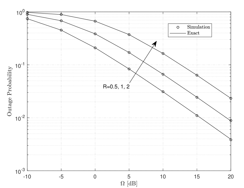
Figure 2: Outage probability versus peak interference to noise power ratio $\Omega$ for $\lambda_{1}=4$, $\lambda_{2}=3$, $\lambda_{0}=\lambda_{3}=1$, and $R=0.5,1,2$.

In Fig. 2, the outage probability is plotted against the peak interference to noise power ratio $\Omega=Q/\sigma^{2}$ for $\lambda_{1}=4$, $\lambda_{2}=3$, $\lambda_{0}=\lambda_{3}=1$, and $R\in\{0.5,1,2\}$. It can be readily observed that the outage probability decreases as $\Omega$ increases. This is rather intuitive, since the PR tolerates higher interference power as $Q$ increases. Accordingly, the ST can adjust its transmit power to a higher level, which results in a lower outage probability.

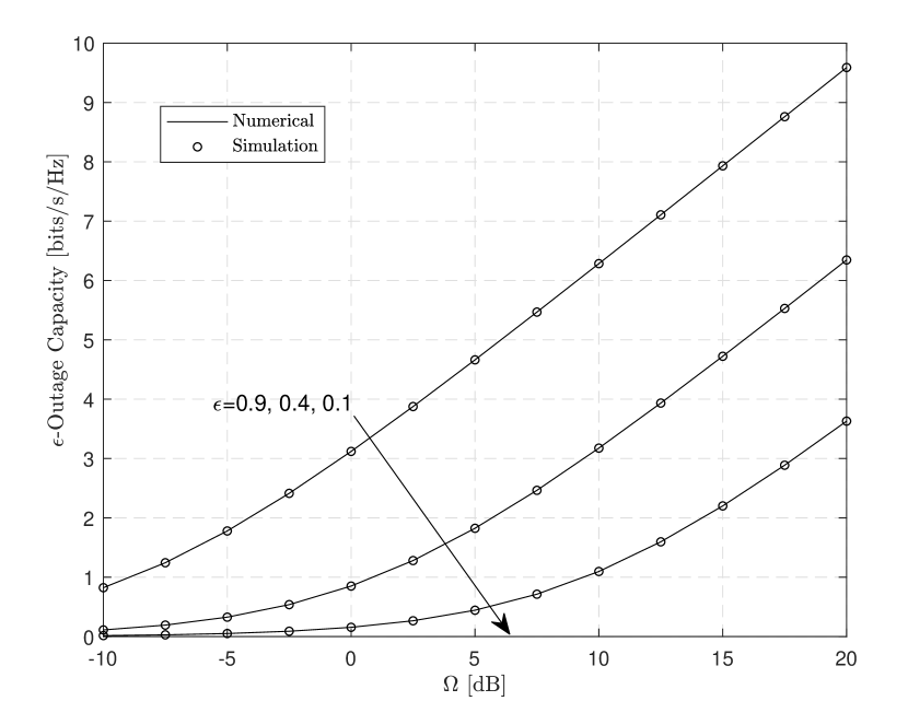
Figure 3: Outage capacity versus peak interference to noise power ratio $\Omega$ for $\lambda_{1}=2$, $\lambda_{2}=3$, $\lambda_{0}=\lambda_{3}=1$, and $\epsilon=0.1,0.4,0.9$.

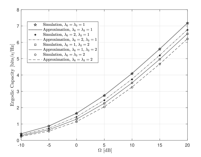
Figure 4: Ergodic capacity versus peak interference to noise power ratio $\Omega$ for $\lambda_{1}=4$, $\lambda_{2}=3$ and different values of $\lambda_{0}$ and $\lambda_{3}$.

In Fig. 3, the $\epsilon$-outage capacity is depicted against $\Omega$ for $\lambda_{1}=2$, $\lambda_{2}=3$, $\lambda_{0}=\lambda_{3}=1$, and $\epsilon\in\{0.1,0.4,0.9\}$. As illustrated, the $\epsilon$-outage capacity of the secondary system improves as $\Omega$ increases.

Fig. 4, illustrates the ergodic capacity as a function of $\Omega$ for $\lambda_{1}=4$, $\lambda_{2}=3$, and different values of $\lambda_{0}$ and $\lambda_{3}$. The analytical curves obtained via the approximations for ergodic capacity obtained earlier in (15) and (16) with $I=N=14$. We note that the approximations for ergodic capacity match perfectly with the Monte Carlo simulations. As expected, the ergodic capacity increases as $\Omega$ increases. However, the ergodic capacity decreases as $\lambda_{0}$ or $\lambda_{3}$ increases. This is due to the fact that as $\lambda_{0}$ or $\lambda_{3}$ increases, the interference power caused by the secondary network to the PR increases, hence, the ST will decrease its transmit power to satisfy the interference constraint at the PR, which consequently decreases the ergodic capacity of the secondary system.

Figure 5: Ergodic capacity versus $\lambda_{1}$ for $\lambda_{0}=0.1$, $\lambda_{3}=1$ and different values of $\Omega$ and $\lambda_{2}$.

In Fig. 5, we investigate the ergodic capacity as a function of $\lambda_{1}$ for $\lambda_{0}=0.1$, $\lambda_{3}=1$, and different values of $\Omega$ and $\lambda_{2}$. The analytical curves obtained via the approximations in (15) and (16). We note that the approximations for the ergodic capacity coincide with the Monte Carlo simulations. Most importantly, we observe that the ergodic capacity initially increases with the increase of $\lambda_{1}$ and then saturates for large vaues of $\lambda_{1}$. In addition, we show that the anayltical and simulation curves for the ergodic capacity approach that obtained in (17) as $\lambda_{1}\to\infty$.

In Fig. 6, we plot the effective capacity as a function of delay QoS exponent $A$ for $\lambda_{1}=2$, $\lambda_{2}=3$, $\lambda_{0}=\lambda_{3}=1$, and different values of $\Omega$. We evaluate the effective capacity using the numerical integration for arbitrary values of $A$ and the analyitcal expressions obtained via the approximations in (22) and (24) for an integer $A$ with $I=N=14$. As demonstrated in the figure, the simulation results confirm the accuracy of the curves obtained through the numerical integration and the approximat expressions.

In Fig. 7, we plot the average BER versus $\Omega$ for various binary modulation formats for $\lambda_{1}=4$, $\lambda_{2}=3$, $\lambda_{0}=0.1$ and $\lambda_{3}=1$. It is evident from the figure that the obtained expression in (26) provides a highly accurate approximation of the BER performance of the seconday system. Finally, we confirmed the correctness of our theoretical analysis, for various system parameters, through simulations.

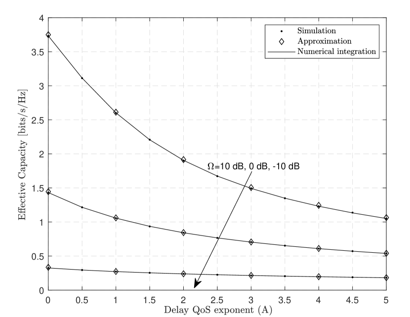
Figure 6: Effective capacity versus delay QoS exponent $A$ for $\lambda_{1}=2$, $\lambda_{2}=3$, $\lambda_{0}=\lambda_{3}=1$, and $\Omega=-10,0,10$ dB.

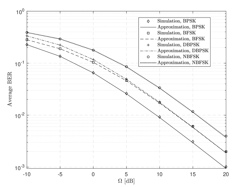
Figure 7: Average BER of various binary modulation formats versus interference to noise power ratio $\Omega$ for $\lambda_{1}=4$, $\lambda_{2}=3$, $\lambda_{0}=0.1$, $\lambda_{3}=1$.

V Conclusion

We proposed an underlay SSBC system in which a secondary BC system shared the spectrum of a primary network. The performance of the secondary BC system is analyzed employing a transmit power adaption strategy at the ST that satisfies the instantaneous interference constraint at the PR. We derived an exact analytical expression for the CDF of the SNR of the secondary system, based on which, we studied the ergodic capacity, effective capacity and average BER. More specifically, we derive novel and accurate analytical approximations for the ergodic and effective capacities, together with the average BER. We further obtained insightful closed-form asymptotic expressions for the aforementioned performance metrics as $\lambda_{1}\to\infty$. For instance, it was evident from the asymptotic ergodic capacity that the performance will initially improve as $\lambda_{1}$ increases and then saturate as $\lambda_{1}$ grows large. Finally, we confirmed the correctness of our theoretical analysis, for various system parameters, through Monte Carlo simulations.

Appendix A
Proof Of Proposition 1

The CDF of the RV $\Upsilon$ in (7) can be expressed as

$$F_{\Upsilon}(\gamma)=\Pr\{\Upsilon\leq\gamma\}=\Pr\bigg{\{}\frac{\Omega|h_{1}|^{2}|h_{2}|^{2}}{|h_{1}|^{2}|h_{3}|^{2}+|h_{0}|^{2}}\leq\gamma\bigg{\}},$$ (32)

where $\Omega={Q}/{\sigma^{2}}$. In veiw of $|h_{i}|^{2}$, $i\in\{0,1,2,3\}$, being independent exponentially distributed RVs with the CDF and PDF given in (1) and (2), respectively, $F_{\Upsilon}(\gamma)$ can be obtained as shown in (33) at the bottom of the page. Utilizing [43, Eq. (3.353.5)] to evaluate $I_{1}$ of (33) below, $F_{\Upsilon}(\gamma)$ can be finally expressed as in (8) after some basic algebraic manipulations.

 

$$\begin{split}F_{\Upsilon}(\gamma)&=\int_{0}^{\infty}\int_{0}^{\infty}\int_{0}^{\infty}\Pr\bigg{\{}|h_{2}|^{2}\leq\frac{\gamma(x_{1}x_{3}+x_{0})}{\Omega x_{1}}\bigg{\}}f_{|h_{0}|^{2}}(x_{0})f_{|h_{1}|^{2}}(x_{1})f_{|h_{3}|^{2}}(x_{3})\ \mathrm{d}x_{0}\ \mathrm{d}x_{1}\ \mathrm{d}x_{3}\\ &=\int_{0}^{\infty}\int_{0}^{\infty}\int_{0}^{\infty}\bigg{(}1-e^{-\frac{\gamma(x_{1}x_{3}+x_{0})}{\Omega\lambda_{2}x_{1}}}\bigg{)}\frac{1}{\lambda_{0}}e^{-\frac{x_{0}}{\lambda_{0}}}\ \frac{1}{\lambda_{1}}e^{-\frac{x_{1}}{\lambda_{1}}}\ \frac{1}{\lambda_{3}}e^{-\frac{x_{3}}{\lambda_{3}}}\ \mathrm{d}x_{0}\ \mathrm{d}x_{1}\ \mathrm{d}x_{3}\\ &=1-\int_{0}^{\infty}\int_{0}^{\infty}\int_{0}^{\infty}e^{-\frac{\gamma(x_{1}x_{3}+x_{0})}{\Omega\lambda_{2}x_{1}}}\ \frac{1}{\lambda_{0}}e^{-\frac{x_{0}}{\lambda_{0}}}\ \frac{1}{\lambda_{1}}e^{-\frac{x_{1}}{\lambda_{1}}}\ \frac{1}{\lambda_{3}}e^{-\frac{x_{3}}{\lambda_{3}}}\ \mathrm{d}x_{0}\ \mathrm{d}x_{1}\ \mathrm{d}x_{3}\\ &=1-\int_{0}^{\infty}\int_{0}^{\infty}\ \bigg{(}\int_{0}^{\infty}e^{-\frac{\gamma x_{0}}{\Omega\lambda_{2}x_{1}}}\ \frac{1}{\lambda_{0}}e^{-\frac{x_{0}}{\lambda_{0}}}\ \mathrm{d}x_{0}\bigg{)}\ e^{-\frac{\gamma x_{3}}{\Omega\lambda_{2}}}\ \frac{1}{\lambda_{1}}e^{-\frac{x_{1}}{\lambda_{1}}}\ \frac{1}{\lambda_{3}}e^{-\frac{x_{3}}{\lambda_{3}}}\ \mathrm{d}x_{1}\ \mathrm{d}x_{3}\\ &=1-\int_{0}^{\infty}\frac{\Omega\lambda_{2}x_{1}}{\Omega\lambda_{2}x_{1}+\lambda_{0}\gamma}\bigg{(}\int_{0}^{\infty}\ e^{-\frac{\gamma x_{3}}{\Omega\lambda_{2}}}\ \frac{1}{\lambda_{3}}e^{-\frac{x_{3}}{\lambda_{3}}}\ \mathrm{d}x_{3}\bigg{)}\frac{1}{\lambda_{1}}e^{-\frac{x_{1}}{\lambda_{1}}}\ \mathrm{d}x_{1}\\ &=1-{\frac{{\Omega}^{2}{{\lambda_{2}}}^{2}}{\Omega{\lambda_{2}}+{\lambda_{3}\gamma}}}\underbrace{\int_{0}^{\infty}{\frac{{x_{1}}}{\Omega{\lambda_{2}x_{1}}+\lambda_{0}\gamma}}\ \frac{1}{\lambda_{1}}e^{-\frac{x_{1}}{\lambda_{1}}}\ \mathrm{d}x_{1}}_{\text{$I_{1}$}}.\\ &=1-{\frac{{\Omega}^{2}{{\lambda_{2}}}^{2}}{\Omega{\lambda_{2}}+{\lambda_{3}\gamma}}}\left(\frac{-\lambda_{0}\gamma E_{1}\left(\frac{\lambda_{0}\gamma}{\Omega\lambda_{1}\lambda_{2}}\right)e^{\frac{\lambda_{0}\gamma}{\Omega\lambda_{1}\lambda_{2}}}+\Omega\lambda_{1}\lambda_{2}}{{\Omega}^{2}{{\lambda_{2}}}^{2}\lambda_{1}}\right).\end{split}$$ (33)

 

Appendix B
Proof Of Proposition 1

Making use of (14) in (12), yields

$$\begin{split}\overline{C}\approx&\frac{1}{\ln(2)}\underbrace{\int_{0}^{\infty}\frac{\Omega\lambda_{2}}{\left(\Omega\lambda_{2}+\lambda_{3}\gamma\right)(1+\gamma)}\,\mathrm{d}\gamma}_{\text{$I_{2}$}}-\frac{4\sqrt{2}\pi a_{N}a_{I}}{\ln(2)}\\ &\times\sum_{n=1}^{N+1}\sum_{i=1}^{I+1}\underbrace{\int_{0}^{\infty}\frac{\sqrt{b_{n}}\lambda_{0}\gamma e^{-\frac{\zeta_{i,n}\lambda_{0}\gamma}{\Omega\lambda_{1}\lambda_{2}}}}{\left(\Omega\lambda_{1}\lambda_{2}+\lambda_{1}\lambda_{3}\gamma\right)(1+\gamma)}\,\mathrm{d}\gamma}_{\text{$I_{3}$}}.\end{split}$$ (34)

Using partial fraction decomposition, $I_{2}$ can be readily obtained as

$$\begin{split}I_{2}&=\frac{\Omega\lambda_{2}}{{\Omega\lambda_{2}-\lambda_{3}}}\int_{0}^{\infty}\left(\frac{-\lambda_{3}}{\Omega\lambda_{2}+\lambda_{3}\gamma}+\frac{1}{1+\gamma}\right)\,\mathrm{d}\gamma\\ &=\frac{\Omega\lambda_{2}\ln\left(\frac{\Omega\lambda_{2}}{\lambda_{3}}\right)}{\Omega\lambda_{2}-\lambda_{3}},\ \ \ \ \Omega\neq\frac{\lambda_{3}}{\lambda_{2}}.\end{split}$$ (35)

Similarly, $I_{3}$ can be expressed as

$$\begin{split}I_{3}=\frac{\sqrt{b_{n}}\lambda_{0}}{{\Omega\lambda_{2}-\lambda_{3}}}&\int_{0}^{\infty}\left(\frac{\Omega\lambda_{2}e^{-\frac{\zeta_{i,n}\lambda_{0}\gamma}{\Omega\lambda_{1}\lambda_{2}}}}{\Omega\lambda_{1}\lambda_{2}+\lambda_{1}\lambda_{3}\gamma}-\frac{e^{-\frac{\zeta_{i,n}\lambda_{0}\gamma}{\Omega\lambda_{1}\lambda_{2}}}}{\lambda_{1}+\lambda_{1}\gamma}\right)\,\mathrm{d}\gamma.\end{split}$$ (36)

Utilizing the integral formula [43, Eq. (3.352.4)], $I_{3}$ can be finally evaluated as

$$\begin{split}I_{3}=\ \frac{\sqrt{b_{n}}\Omega\lambda_{0}\lambda_{2}\ e^{\frac{\lambda_{0}\zeta_{i,n}}{\lambda_{1}\lambda_{3}}}E_{1}\left(\frac{\lambda_{0}\zeta_{i,n}}{\lambda_{1}\lambda_{3}}\right)}{\lambda_{1}\lambda_{3}\left(\Omega\lambda_{2}-\lambda_{3}\right)}-\frac{\sqrt{b_{n}}\lambda_{0}e^{\frac{\lambda_{0}\zeta_{i,n}}{\Omega\lambda_{1}\lambda_{2}}}E_{1}\left(\frac{\lambda_{0}\zeta_{i,n}}{\Omega\lambda_{1}\lambda_{2}}\right)}{\lambda_{1}\left(\Omega\lambda_{2}-\lambda_{3}\right)},\end{split}$$ (37)

where $\lambda_{3}\neq\Omega\lambda_{2}$. Substituting (35) and (37) into (34), after some basic algebraic manipulations, yields the desired result in (15). The ergodic capacity of the secondary system for the special case $\lambda_{3}=\Omega\lambda_{2}$ can be obtained by substituting $\lambda_{3}=\Omega\lambda_{2}$ in (34). Accordingly,

$$\begin{split}\overline{C}\approx&\frac{1}{\ln(2)}\int_{0}^{\infty}\frac{1}{\left(1+\gamma\right)^{2}}\,\mathrm{d}\gamma\\ &-\frac{4\sqrt{2}\pi a_{N}a_{I}\lambda_{0}}{\Omega\lambda_{1}\lambda_{2}\ln(2)}\sum_{n=1}^{N+1}\sum_{i=1}^{I+1}\int_{0}^{\infty}\frac{\sqrt{b_{n}}\gamma e^{-\frac{\zeta_{i,n}\lambda_{0}\gamma}{\Omega\lambda_{1}\lambda_{2}}}}{(1+\gamma)^{2}}\,\mathrm{d}\gamma\\ =&\frac{1}{\ln(2)}-\frac{4\sqrt{2}\pi a_{N}a_{I}\lambda_{0}}{\Omega\lambda_{1}\lambda_{2}\ln(2)}\sum_{n=1}^{N+1}\sum_{i=1}^{I+1}\left(\int_{0}^{\infty}\frac{\sqrt{b_{n}}e^{-\frac{\zeta_{i,n}\lambda_{0}\gamma}{\Omega\lambda_{1}\lambda_{2}}}}{1+\gamma}\right.\\ &\left.\ \ \ \ \ \ \ \ \ \ \ \ \ \ \ \ \ \ \ \ \ \ \ \ \ \ \ \ \ \ \ \ \ \ \ \ -\int_{0}^{\infty}\frac{\sqrt{b_{n}}e^{-\frac{\zeta_{i,n}\lambda_{0}\gamma}{\Omega\lambda_{1}\lambda_{2}}}}{(1+\gamma)^{2}}\right).\end{split}$$ (38)

Utilizing the identities [43, Eq. (3.352.4)] and [43, Eq. (3.353.2)] to evaluate the involved integrals above, after some algebraic manipulations, $\overline{C}$ is finally as expressed in (16).

Appendix C
Proof Of Proposition 3

Making use of (14) in the integral of (20), yields

$$\begin{split}\int_{0}^{\infty}\frac{1-F_{\Upsilon}(\gamma)}{\left(1+\gamma\right)^{A+1}}\approx&\underbrace{\int_{0}^{\infty}\frac{\Omega\lambda_{2}}{\left(\Omega\lambda_{2}+\lambda_{3}\gamma\right)(1+\gamma)^{A+1}}\,\mathrm{d}\gamma}_{\text{$\Xi_{1}$}}\\ -4\sqrt{2}\pi a_{N}a_{I}\sum_{n=1}^{N+1}&\sum_{i=1}^{I+1}\underbrace{\int_{0}^{\infty}\frac{\sqrt{b_{n}}\lambda_{0}\gamma e^{-\frac{\zeta_{i,n}\lambda_{0}\gamma}{\Omega\lambda_{1}\lambda_{2}}}}{\left(\Omega\lambda_{1}\lambda_{2}+\lambda_{1}\lambda_{3}\gamma\right)(1+\gamma)^{A+1}}\,\mathrm{d}\gamma}_{\text{$\Xi_{2}$}}.\end{split}$$ (39)

$\Xi_{1}$ can be evaluated with the help [43, Eq. (3.227.1)] as

$$\Xi_{1}=\frac{\Omega\lambda_{2}}{\lambda_{3}(A+1)}\ {}_{2}F_{1}\left(A+1;1;A+2;1-\frac{\Omega\lambda_{2}}{\lambda_{3}}\right).$$ (40)

It is not tractable to find a closed-form expression for $\Xi_{2}$ above for an arbitrary $A$. However, it is possible to find a closed-form for $\Xi_{2}$ when $A$ is an integer. Applying partial fraction decomposition, $\Xi_{2}$ can be expressed as

$$\begin{split}\Xi_{2}=&\int_{0}^{\infty}\frac{\sqrt{b_{n}}\lambda_{0}c_{0}e^{-\frac{\zeta_{i,n}\lambda_{0}\gamma}{\Omega\lambda_{1}\lambda_{2}}}}{\left(\Omega\lambda_{2}-\lambda_{3}\right)^{A+1}\left(\gamma+\frac{\Omega\lambda_{2}}{\lambda_{3}}\right)}\,\mathrm{d}\gamma\\ &+\sum_{k=1}^{A+1}\int_{0}^{\infty}\frac{\sqrt{b_{n}}\lambda_{0}c_{k}e^{-\frac{\zeta_{i,n}\lambda_{0}\gamma}{\Omega\lambda_{1}\lambda_{2}}}}{\left(\Omega\lambda_{2}-\lambda_{3}\right)^{A+2-k}\left(\gamma+1\right)^{k}}\,\mathrm{d}\gamma,\end{split}$$ (41)

where $c_{k}$, $k=0,1,...,A+1$ are constants. Utilizing [43, Eq. (3.352.4)] and [43, Eq. (3.382.4)], after some algebraic manipulations, $\Xi_{2}$ can be evaluated as

$$\begin{split}\Xi_{2}=&\frac{\sqrt{b_{n}}\lambda_{0}c_{0}E_{1}\left(\frac{\lambda_{0}\zeta_{i,n}}{\lambda_{1}\lambda_{3}}\right)e^{\frac{\lambda_{0}\zeta_{i,n}}{\lambda_{1}\lambda_{3}}}}{\left(\Omega\lambda_{2}-\lambda_{3}\right)^{A+1}}\\ &+\sum_{k=1}^{A+1}\frac{\sqrt{b_{n}}\lambda_{0}c_{k}\left(\frac{\lambda_{0}\zeta_{i,n}}{\Omega\lambda_{1}\lambda_{2}}\right)^{k-1}}{\left(\Omega\lambda_{2}-\lambda_{3}\right)^{A+2-k}}\Gamma\left(-k+1,\frac{\lambda_{0}\zeta_{i,n}}{\Omega\lambda_{1}\lambda_{2}}\right)e^{\frac{\lambda_{0}\zeta_{i,n}}{\Omega\lambda_{1}\lambda_{2}}},\end{split}$$ (42)

where $\lambda_{3}\neq\Omega\lambda_{2}$ and $A$ is an integer. Making use of (40), (42) and (39) in (20) yields the desired result in (21). However, the effective capacity of the secondary system for the special case when $\lambda_{3}=\Omega\lambda_{2}$ can be obtained by substituting $\lambda_{3}=\Omega\lambda_{2}$ in (39). Accordingly,

$$\begin{split}\int_{0}^{\infty}\frac{1-F_{\Upsilon}(\gamma)}{\left(1+\gamma\right)^{A+1}}\,\,\mathrm{d}\gamma=&\int_{0}^{\infty}\frac{1}{\left(1+\gamma\right)^{A+2}}\,\mathrm{d}\gamma\\ -\frac{4\sqrt{2}\pi a_{N}a_{I}\lambda_{0}}{\Omega\lambda_{1}\lambda_{2}}&\sum_{n=1}^{N+1}\sum_{i=1}^{I+1}\underbrace{\int_{0}^{\infty}\frac{\sqrt{b_{n}}\gamma e^{-\frac{\zeta_{i,n}\lambda_{0}\gamma}{\Omega\lambda_{1}\lambda_{2}}}}{\left(1+\gamma\right)^{A+2}}\,\mathrm{d}\gamma}_{\text{$\Xi_{3}$}}.\end{split}$$ (43)

$\Xi_{3}$ can be evaluated with the help [47, Eq. (39)] as

$$\begin{split}\Xi_{3}=\sqrt{b_{n}}\textit{U}\left(2;1-A;\frac{\zeta_{i,n}\lambda_{0}}{\Omega\lambda_{1}\lambda_{2}}\right).\end{split}$$ (44)

Making use of (43) and (44) in (20) yields the desired result in (22).

Appendix D
Proof Of Proposition 4

Using integration by parts, $\overline{P_{e}}(p,q)$ in (25) can be expressed as

$$\begin{split}\overline{P_{e}}(p,q)=\frac{q^{p}}{2\Gamma(p)}\int_{0}^{\infty}e^{-q\gamma}\gamma^{p-1}F_{\Upsilon}(\gamma)\,\mathrm{d}\gamma.\end{split}$$ (45)

Making use of (14) in (45), yields

$$\begin{split}\overline{P_{e}}(p,q)\approx&\frac{q^{p}}{2\Gamma(p)}\int_{0}^{\infty}\frac{\lambda_{3}e^{-q\gamma}\gamma^{p}}{\Omega\lambda_{2}+\gamma\lambda_{3}}\,\mathrm{d}\gamma+\frac{4\sqrt{2}\pi a_{N}a_{I}q^{p}}{2\Gamma(p)}\\ &\times\sum_{n=1}^{N+1}\sum_{i=1}^{I+1}\int_{0}^{\infty}\frac{\sqrt{b_{n}}\lambda_{0}e^{-\frac{\zeta_{i,n}\lambda_{0}\gamma}{\Omega\lambda_{1}\lambda_{2}}}\gamma^{p}e^{-q\gamma}}{\Omega\lambda_{1}\lambda_{2}+\gamma\lambda_{1}\lambda_{3}}\,\mathrm{d}\gamma.\end{split}$$ (46)

Utilizing [43, Eq. (3.383.10)] to evaluate the involved intgerals above, after basic algebric manipulations, $\overline{P_{e}}$ is finally as expressed in (26).

References

- [1] F. Boccardi, R. W. Heath, A. Lozano, T. L. Marzetta, and P. Popovski, “Five disruptive technology directions for 5G,” IEEE Communications Magazine, vol. 52, no. 2, pp. 74–80, Feb. 2014.
- [2] S. Dang, O. Amin, B. Shihada, and M.-S. Alouini, “What should 6G be?” Nature Electronics, vol. 3, no. 1, pp. 20–29, 2020.
- [3] I. Analytics, “Internet of things (IoT) active device connections installed base worldwide from 2015 to 2025,” https://www.statista.com/statistics/1101442/iot-number-of-connected-devices-worldwide/, Aug. 2018.
- [4] M. Chiani and A. Elzanaty, “On the LoRa modulation for IoT: Waveform properties and spectral analysis,” IEEE Internet of Things Journal, vol. 6, no. 5, pp. 8463–8470, Oct. 2019.
- [5] U. Raza, P. Kulkarni, and M. Sooriyabandara, “Low power wide area networks: An overview,” IEEE Communications Surveys & Tutorials, vol. 19, no. 2, pp. 855–873, 2017.
- [6] D. Pianini, A. Elzanaty, A. Giorgetti, and M. Chiani, “Distributed programming paradigm for cyber-physical systems over LoRaWANs,” in IEEE Int. Conf. on Global Comm. (GLOBECOM), Abu Dhabi, United Arab Emirates, Dec. 2018.
- [7] F. Rezaei, C. Tellambura, and S. Herath, “Large-scale wireless-powered networks with backscatter communications—a comprehensive survey,” IEEE Open Journal of the Communications Society, vol. 1, pp. 1100–1130, July 2020.
- [8] N. Van Huynh, D. T. Hoang, X. Lu, D. Niyato, P. Wang, and D. I. Kim, “Ambient backscatter communications: A contemporary survey,” IEEE Communications Surveys & Tutorials, vol. 20, no. 4, pp. 2889–2922, May 2018.
- [9] G. Wang, F. Gao, R. Fan, and C. Tellambura, “Ambient backscatter communication systems: Detection and performance analysis,” IEEE Transactions on Communications, vol. 64, no. 11, pp. 4836–4846, 2016.
- [10] V. Liu, A. Parks, V. Talla, S. Gollakota, D. Wetherall, and J. R. Smith, “Ambient backscatter: Wireless communication out of thin air,” ACM SIGCOMM Computer Communication Review, vol. 43, no. 4, pp. 39–50, 2013.
- [11] Y. W. Chen, R. Zhang, C. W. Hsu, and G. K. Chang, “Key enabling technologies for the post-5G era: Fully adaptive, all-spectra coordinated radio access network with function decoupling,” IEEE Communications Magazine, vol. 58, no. 9, pp. 60–66, 2020.
- [12] E. Hossain and K. Thilina, “Chapter 13 - cognitive radio networks and spectrum sharing,” in Academic Press Library in Mobile and Wireless Communications, S. K. Wilson, S. Wilson, and E. Biglieri, Eds. Oxford: Academic Press, 2016, pp. 467 – 522.
- [13] Y. H. Al-Badarneh, C. N. Georghiades, and M.-S. Alouini, “Asymptotic performance analysis of generalized user selection for interference-limited multiuser secondary networks,” IEEE Transactions on Cognitive Communications and Networking, vol. 5, no. 1, pp. 82–92, Jan. 2019.
- [14] S. Lee, R. Zhang, and K. Huang, “Opportunistic wireless energy harvesting in cognitive radio networks,” IEEE Transactions on Wireless Communications, vol. 12, no. 9, pp. 4788–4799, Aug. 2013.
- [15] D. T. Hoang, D. Niyato, P. Wang, D. I. Kim, and Z. Han, “Ambient backscatter: A new approach to improve network performance for RF-powered cognitive radio networks,” IEEE Transactions on Communications, vol. 65, no. 9, pp. 3659–3674, Sept. 2017.
- [16] Y. Liu, G. Wang, Z. Dou, and Z. Zhong, “Coding and detection schemes for ambient backscatter communication systems,” IEEE Access, vol. 5, pp. 4947–4953, 2017.
- [17] C. Boyer and S. Roy, “Coded QAM backscatter modulation for RFID,” IEEE Transactions on Communications, vol. 60, no. 7, pp. 1925–1934, May 2012.
- [18] X. Lu, H. Jiang, D. Niyato, D. I. Kim, and Z. Han, “Wireless-powered device-to-device communications with ambient backscattering: Performance modeling and analysis,” IEEE Transactions on Wireless Communications, vol. 17, no. 3, pp. 1528–1544, 2018.
- [19] J. Qian, F. Gao, G. Wang, S. Jin, and H. Zhu, “Noncoherent detections for ambient backscatter system,” IEEE Transactions on Wireless Communications, vol. 16, no. 3, pp. 1412–1422, 2017.
- [20] ——, “Semi-coherent detection and performance analysis for ambient backscatter system,” IEEE Transactions on Communications, vol. 65, no. 12, pp. 5266–5279, 2017.
- [21] G. Yang, Y. Liang, R. Zhang, and Y. Pei, “Modulation in the air: Backscatter communication over ambient OFDM carrier,” IEEE Transactions on Communications, vol. 66, no. 3, pp. 1219–1233, 2018.
- [22] M. A. ElMossallamy, M. Pan, R. Jäntti, K. G. Seddik, G. Y. Li, and Z. Han, “Noncoherent backscatter communications over ambient OFDM signals,” IEEE Transactions on Communications, vol. 67, no. 5, pp. 3597–3611, 2019.
- [23] D. Darsena, G. Gelli, and F. Verde, “Modeling and performance analysis of wireless networks with ambient backscatter devices,” IEEE Transactions on Communications, vol. 65, no. 4, pp. 1797–1814, 2017.
- [24] W. Zhao, G. Wang, R. Fan, L. Fan, and S. Atapattu, “Ambient backscatter communication systems: Capacity and outage performance analysis,” IEEE Access, vol. 6, pp. 22 695–22 704, April 2018.
- [25] Y. H. Al-Badarneh, M. S. Alouini, and C. N. Georghiades, “Performance analysis of monostatic multi-tag backscatter systems with general order tag selection,” IEEE Wireless Communications Letters, vol. 9, no. 8, pp. 1201–1205, 2020.
- [26] X. Zhou, G. Wang, Y. Wang, and J. Cheng, “An approximate BER analysis for ambient backscatter communication systems with tag selection,” IEEE Access, vol. 5, pp. 22 552–22 558, 2017.
- [27] D. T. Hoang, D. Niyato, P. Wang, D. I. Kim, and Z. Han, “The tradeoff analysis in RF-powered backscatter cognitive radio networks,” in IEEE Global Communications Conference (GLOBECOM), Feb. 2016, pp. 1–6.
- [28] D. T. Hoang, D. Niyato, P. Wang, D. I. Kim, and L. B. Le, “Overlay RF-powered backscatter cognitive radio networks: A game theoretic approach,” in IEEE International Conference on Communications (ICC), 2017, pp. 1–6.
- [29] R. Kishore, S. Gurugopinath, P. C. Sofotasios, S. Muhaidat, and N. Al-Dhahir, “Opportunistic ambient backscatter communication in RF-powered cognitive radio networks,” in 2019 IEEE Wireless Communications and Networking Conference (WCNC), 2019, pp. 1–6.
- [30] H. Guo, R. Long, and Y.-C. Liang, “Cognitive backscatter network: A spectrum sharing paradigm for passive IoT,” IEEE Wireless Communications Letters, vol. 8, no. 5, pp. 1423–1426, Oct. 2019.
- [31] Y. C. Liang, Q. Zhang, E. G. Larsson, and G. Y. Li, “Symbiotic radio: Cognitive backscattering communications for future wireless networks,” IEEE Transactions on Cognitive Communications and Networking, pp. 1–1, 2020.
- [32] M. Di Renzo, M. Debbah, D.-T. Phan-Huy, A. Zappone, M.-S. Alouini, C. Yuen, V. Sciancalepore, G. C. Alexandropoulos, J. Hoydis, H. Gacanin, J. de Rosny, A. Bounceu, G. Lerosey, and M. Fink, “Smart radio environments empowered by reconfigurable AI meta-surfaces: an idea whose time has come,” EURASIP J. Wireless Commun. Net., vol. 2019, no. 1, pp. 1–20, May 2019.
- [33] A. Elzanaty, A. Guerra, F. Guidi, and M.-S. Alouini, “Reconfigurable intelligent surfaces for localization: Position and orientation error bounds,” arXiv preprint arXiv:2009.02818, 2020.
- [34] Q. Zhang, Y.-C. Liang, and H. V. Poor, “Large intelligent surface/antennas (LISA) assisted symbiotic radio for IoT communications,” arXiv preprint arXiv:2002.00340, 2020.
- [35] M. Abramowitz and I. A. Stegun, Handbook of Mathematical Functions: with Formulas, Graphs, and Mathematical Tables, Ninth ed. NY, Dover, 1970.
- [36] J. Proakis and M. Salehi, Digital Communications. McGraw-Hill, 2008.
- [37] D. Tse and P. Viswanath, Fundamentals of wireless communication. Cambridge university press, 2005.
- [38] A. A. Alkheir and M. Ibnkahla, “An accurate approximation of the exponential integral function using a sum of exponentials,” IEEE Communications Letters, vol. 17, no. 7, pp. 1364–1367, 2013.
- [39] D. Wu and R. Negi, “Effective capacity: A wireless link model for support of quality of service,” IEEE Transactions on Wireless Communications, vol. 2, no. 4, pp. 630–643, July 2003.
- [40] L. Liu and J. Chamberland, “On the effective capacities of multiple-antenna Gaussian channels,” in 2008 IEEE International Symposium on Information Theory, 2008, pp. 2583–2587.
- [41] Y. H. Al-Badarneh, C. N. Georghiades, and C. E. Mejia, “On the effective rate of MISO/TAS systems in rayleigh fading,” in IEEE International Symposium on Information Theory (ISIT), 2017, pp. 2328–2332.
- [42] G. P. Karatza, K. P. Peppas, and N. C. Sagias, “Effective capacity of multisource multidestination cooperative systems under cochannel interference,” IEEE Transactions on Vehicular Technology, vol. 67, no. 9, pp. 8411–8421, 2018.
- [43] A. Jeffrey and D. Zwillinger, Table of integrals, series, and products. Academic Press, 2007.
- [44] A. Wojnar, “Unknown bounds on performance in Nakagami channels,” IEEE Transactions on Communications, vol. 34, no. 1, pp. 22–24, 1986.
- [45] I. S. Ansari, S. Al-Ahmadi, F. Yilmaz, M. Alouini, and H. Yanikomeroglu, “A new formula for the BER of binary modulations with dual-branch selection over generalized-k composite fading channels,” IEEE Transactions on Communications, vol. 59, no. 10, pp. 2654–2658, 2011.
- [46] M. K. Simon and M.-S. Alouini, Digital communication over fading channels. New York, NY, USA: John Wiley & Sons, 2005, vol. 95.
- [47] M. Kang and M. S. Alouini, “Capacity of MIMO rician channels,” IEEE Transactions on Wireless Communications, vol. 5, no. 1, pp. 112–122, Jan 2006.