AINet: Association Implantation for Superpixel Segmentation

Abstract

Recently, some approaches are proposed to harness deep convolutional networks to facilitate superpixel segmentation. The common practice is to first evenly divide the image into a pre-defined number of grids and then learn to associate each pixel with its surrounding grids. However, simply applying a series of convolution operations with limited receptive fields can only implicitly perceive the relations between the pixel and its surrounding grids. Consequently, existing methods often fail to provide an effective context when inferring the association map. To remedy this issue, we propose a novel Association Implantation (AI) module to enable the network to explicitly capture the relations between the pixel and its surrounding grids. The proposed AI module directly implants the features of grid cells to the surrounding of its corresponding central pixel, and conducts convolution on the padded window to adaptively transfer knowledge between them. With such an implantation operation, the network could explicitly harvest the pixel-grid level context, which is more in line with the target of superpixel segmentation comparing to the pixel-wise relation. Furthermore, to pursue better boundary precision, we design a boundary-perceiving loss to help the network discriminate the pixels around boundaries in hidden feature level, which could benefit the subsequent inferring modules to accurately identify more boundary pixels. Extensive experiments on BSDS500 and NYUv2 datasets show that our method could not only achieve state-of-the-art performance but maintain satisfactory inference efficiency. Our code is available at https://github.com/wangyxxjtu/AINet-ICCV2021.

1 Introduction

Superpixels are image regions formed by grouping image pixels similar in color and other low-level properties, which could be viewed as an over-segmentation of image. The process of extracting superpixels is known as superpixel segmentation. Comparing to pixels, superpixel provides a more effective representation for image data. With such a compact representation, the computational efficiency of vision algorithms could be improved [18, 11, 36]. Consequently, superpixel could benefit many vision tasks like semantic segmentation [12, 40, 43], object detection [9, 30], optical flow estimation [14, 25, 34, 39], and even adversarial attack [7]. In light of the fundamental importance of superpixels in computer vision, superpixel segmentation attracts much attention since it is first introduced by Ren and Malik [28] in 2003.

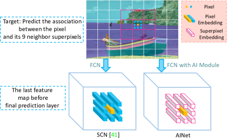
Figure 1: Different from the SCN [41] that implicitly learns the association using the cascaded convolutions, our AINet proposes to implant the corresponding grid features to the surrounding of the pixel to explicitly perceive the relation between each pixel and its neighbor grids.

The common practice for superpixel segmentation is to first split the image into grid cells and then estimate the membership of each pixel to its adjacent cells, by which the grouping could be performed. Meanwhile, the membership estimation plays the key role in superpixel segmentation. Traditional approaches usually utilize the hand-craft features and estimate the relevance of pixel to its neighbor cells based on clustering or graph-based methods [1, 24, 20, 22, 2], however, these methods all suffer from the weakness of the hand-craft features and are difficult to integrate into other trainable deep frameworks. Inspired by the success of deep neural networks in many computer version problems, researchers recently attempts to adopt the deep learning technique to superpixel segmentation [15, 41, 37]. As mentioned in abstract, previous deep methods attempt to assign pixels by learning the association of each pixel to its surrounding grids using the fully convolutional networks [31]. The popular solutions like SCN [41], SSN [15] employ the U-net architecture [29] to predict the association, , the 9-way probabilities, for each pixel. Although stacking convolution layers can enlarge the receptive field and help study the pixel-grid wise probabilities, introducing low-level features with skip connection in the final layer will pollute the probabilities due to the added pixel-pixel wise information, since the ultimate target is to predict the association between the target pixel and its 9-neighbor grids instead of its 9-neighbor pixels.

To tackle this weakness, we propose to directly implant the grid features to the surrounding of the corresponding pixel using an association implantation (AI) module. Fig. 1 simply shows the core idea of our AI module, before feeding the last features into the prediction layer, our AI module is performed: for each pixel, we place the corresponding grid features to its neighbors, then a convolution with $3\times 3$ kernel is followed, this convolution is no longer to capture the pixel-pixel relation but the relation between pixel and its 9 neighbor grids, providing the consistent context with the target of Sp Seg. Our proposed AI module provides a simple and intuitive way to allow the network to harvest the pixel-neighbor cells context in an explicit fashion, which is exactly required by superpixel segmentation. Comparing to existing methods, such a design is more consistent with the target of superpixel segmentation and could give more beneficial support for the subsequent association map inferring.

Besides, a satisfactory superpixel algorithm should acctually identify the boundary pixels, however, some designs towards this target still missed among existing works. To pursue better boundary precision, we augment the optimization with a boundary-perceiving loss. To be specific, we first sample a set of small local patches on the pixel embedding map along the boundaries. Then, the features with the same/different labels in each patch are treated as the positive/negative samples, on which a classification procedure is performed to enhance the compactness of the features with the same label while distinguish the different semantic features. Our boundary-perceiving loss encourages the model to pay more attention to discriminate the features around boundaries, consequently, more boundary pixels could be identified.

Quantitative and qualitative results on BSDS500 [3] and NYUv2 [32] datasets demonstrate that the proposed method achieves more outstanding performance against the state-of-the-art superpixel segmentation methods. In summary, we make the following contributions in this work:

• We propose a novel AI module to directly capture the relation between the pixel and its surrounding grid cells, such a design builds a more consistent architecture with the target of superpixel segmentation.

• A boundary-perceiving loss is designed to discriminate the features with different semantic labels around boundaries, which could help the network accurately identify boundary pixels and improve the boundary precision.

2 Related Work

Superpixel Segmentation Superpixel segmentation is a well-defined problem and has a long line of research [33, 26, 19, 38, 5, 16]. Traditional superpixel algorithms can be broadly classified into graph-based and clustering-based approaches. Graph-based methods consider the pixels as nodes and the edges as strength of connectivity between adjacent pixels, respectively. Consequently, the superpixel segmentation could be formulated as a graph-partitioning problem. Wide-used algorithms, Felzenszwalb and Huttenlocher (FH) [8] and the entropy rate superpixels (ERS) [22], belong to this category. On the other hand, clustering-based approaches utilize classic clustering techniques like $k$-means to compute the connectivity between the anchor pixels and its neighbors. Well-known methods in this category include SLIC [1], LSC [20], Manifold-SLIC [24] and SNIC [2]. Inspired by the success of deep learning techniques, recently, researchers attempt to utilize the deep neural network to learn the membership of each pixel to its surrounding grid cells. Jampani et al. [15] develop the first differentiable deep network motivated by the classic SLIC method, and Yang et al. [41] further simplify the framework and contribute a more efficient model.

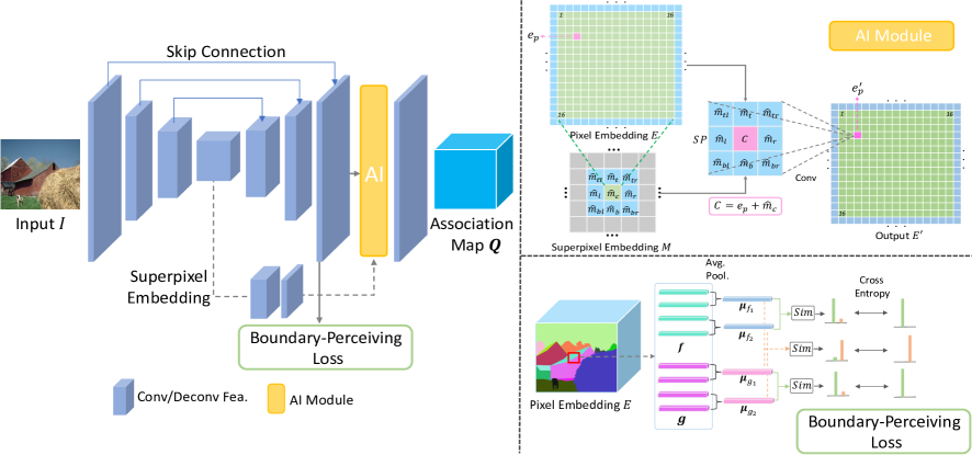
Figure 2: The framework of our AINet. The network takes an image as input and outputs the association map. Meanwhile, the superpixel embedding and pixel embedding are first obtained by the convolutions and then fed into the AI module to obtain the pixel-superpixel context. And the local patch loss is performed on the pixel-wise embeddings to boost the boundary precision. In AI module, the sampling interval is set to 16, and each block indicates a pixel or superpixel embedding.

Application of Superpixel The pre-computed superpixel segmentation could be viewed as a type of weak label or prior knowledge to benefit many downstream tasks, it could be integrated into deep learning pipeline to provide guidance so that some important image properties (e.g., boundaries) could be better preserved [10, 35, 42, 4, 21]. For example, KwaK et al. [18] utilize the superpixel segmentation to perform a region-wise pooling to make the pooled feature have better semantic compactness. In  [27], Cheng et al.consider the superpixel as pseudo label and attempt to boost the image segmentation by identifying more semantic boundary. Besides benefiting the image segmentation or feature pooling, superpixel also provides flexible ways to represent the image data. He et al. [13] convert 2D images patterns into 1D sequential representation, such a novel representation allows the deep network to explore the long-range context of the image. Liu et al. [23] learn the similarity between different superpixels, the developed framework could produce different grained segmentation regions by merging the superpixels according to the learned superpixel similarity.

3 Preliminaries

Before delving into the details of our method, we first introduce the framework of deep-learning based superpixel segmentation, which is also the fundamental theory of this paper. As illustrated in Fig. 1, the image $I$ is partitioned into blocks using a regular size grid, and the grid cell is regarded as the initial superpixel seed. For each pixel $p$ in image $I$, the superpixel segmentation aims at finding a mapping that assigns each pixel to one of its surrounding seeds, 9 neighbors, just as shown in Fig. 1. Mathematically, deep-learning based method feeds the image $I\in\mathcal{R}^{H\times W\times 3}$ to convolution neural network and output an association map $Q\in\mathcal{R}^{H\times W\times 9}$, which indicates the probability of each pixel to its neighbor cells [15, 41]. Since there is no ground-truth for such an output, the supervision for network training is performed in an indirect fashion: the predicted association map $Q$ serves as the intermediate variable to reconstruct the pixel-wise property $l(p)$ like semantic label, position vector, and so on. Consequently, there are two critical steps in training stage.

Step1: Estimate the superpixel property from the surrounding pixels:

$$h(s)=\frac{\sum_{p:s\in N_{p}}{l(p)\cdot q(p,s)}}{\sum_{p:s\in N_{p}}q(p,s)}.$$ (1)

Step2: Reconstruct the pixel property according to the superpixel neighbors:

$$l^{{}^{\prime}}(p)=\sum_{s\in N_{p}}h(s)\cdot q(p,s),$$ (2)

where the $N_{p}$ is the set of adjacent superpixels of $p$, $q(p,s)$ indicates the probability of pixel $p$ assigned to superpixel $s$. Thus, the training loss is to optimize the distance between the ground-truth property and the reconstructed one:

$$\mathcal{\bm{L}}(Q)=\sum_{p}dist(l(p),l^{{}^{\prime}}(p))).$$ (3)

Following Yang’s practice [41], the properties of pixels in this paper include the semantic label and the position vector, , two-dimension spatial coordinates, which are optimized by the cross-entropy loss and the $\mathcal{L}_{2}$ reconstruction loss, respectively.

4 Methodology

An overview of our proposed AINet is shown in Fig. 2. In general, the overall architecture is an encoder-decoder style paradigm, the encoder module compresses the input image and outputs a feature map called superpixel embedding, whose pixels exactly encode the features of grid cells. Subsequently, the superpixel embedding is further fed into the decoder module to produce the association map. Meanwhile, the superpixel embedding and the pixel embedding in decoding stage are integrated to perform the association implantation, and the boundary-perceiving loss also acts on the pixel embedding. Hereinafter, we elaborate the details of our proposed AI module and boundary-perceiving loss.

4.1 Association Implantation Module

To enable the network to explicitly perceive the relation between each pixel and its surrounding grid cells, this work proposes an association implantation module to perform a direct interaction between the pixel and its neighbor cells. As shown in the top right of Fig. 2, we first obtain the embeddings of superpixels and pixels by the convolution network. Then, for each pixel embedding, the corresponding neighbor superpixel features are picked and implanted to its surrounding. Finally, a convolution with kernel size $3\times 3$ is conducted on the expanded pixel embedding to achieve the knowledge propagation.

Formally, let $e_{p}\in\mathcal{R}^{D}$ be the embedding of pixel $p$ from the pixel embedding $E\in\mathcal{R}^{H\times W\times D}$, which is obtained by the deep neural network as shown in Fig. 2. To obtain the embeddings of the grid cells, , superpixel embedding, we compress the input image by $\log_{\text{2}}S$ times using multiple convolutions and max-pooling operations, where $S$ is the sampling interval for the grid cell. For example, if the sampling interval is 16, then, we downsample the image 4 times. This would result in a feature map $M\in\mathcal{R}^{h\times w\times D^{{}^{\prime}}}$ whose pixels exactly encode the features of grid cells, where $h=H/S,\text{and }w=W/S$. To perform the implantation operation on the pixel embedding, we first adjust the channels of $M$ using two $3\times 3$ convolutions, producing a new map $\hat{M}\in\mathcal{R}^{H\times W\times D}$. Then, for the pixel $p$, we pick up its 9 adjacent superpixel embeddings from left to right and top down: $\{\hat{m}_{tl},\hat{m}_{t},\hat{m}_{tr},\hat{m}_{l},\hat{m}_{c},\hat{m}_{r},\hat{m}_{bl},\hat{m}_{b},\hat{m}_{br}\}$ from $\hat{M}$. To allow the network could explicitly capture the relation between pixel $p$ and its neighbor cells, we directly implant the superpixel embeddings into the surrounding of the pixel $p$ to provide pixel-superpixel context:

$$SP=\left[\begin{matrix}\hat{m}_{tl}&\hat{m}_{t}&\hat{m}_{tr}\\ \hat{m}_{l}&\hat{m}_{c}+e_{p}&\hat{m}_{r}\\ \hat{m}_{bl}&\hat{m}_{b}&\hat{m}_{br}\end{matrix}\right].$$ (4)

It is worth noting that the pixels in the same initial grid would share the same surrounding superpixels, since they would degrade into one element in superpixel view. We then adopt a $3\times 3$ convolution to adaptively distill information from the expanded window to benefit the subsequent association map inferring:

$$e^{{}^{\prime}}_{p}=\sum_{ij}SP_{ij}\times w_{ij}+b,$$ (5)

where $w$ and $b$ are the convolution weight and bias, respectively. We traverse all of the pixel embeddings in $E$ and apply the operations in Eq. 4- 5, thus, we could obtain a new pixel embedding $E^{{}^{\prime}}$ whose elements capture the pixel-superpixel level context. In the following, the feature map $E^{{}^{\prime}}$ is fed through a convolution layer to predict the association map $Q$.

As shown in Eq. 4- 5, our AI module directly places the neighbor cell embeddings in the surrounding of the pixel to provide the context required by superpixel segmentation, which is an intuitive and reasonable solution. Comparing to the existing methods that use the stacked convolutions to accumulate the pixel-wise relation, the pixel-superpixel context captured by our AI module is more in line with the target of superpixel segmentation.

4.2 Boundary-Perceiving Loss

Our boundary-perceiving loss is proposed to help the network appropriately assign the pixels around boundaries. As shown in the bottom right of Fig. 2, we first sample a series of patches with a certain size (5$\times$5, for example) around boundaries in the pixel embedding map, and then a classification procedure is conducted to improve the discrimination of the different semantic features.

Formally, let $E\in\mathcal{R}^{H\times W\times D}$ be the pixel-wise embedding map, since the ground-truth label is available during training stage, we could sample a local patch $B\in\mathcal{R}^{K\times K\times D}$ surrounding a pixel in the semantic boundary. For the sake of simplification, the patch $B$ only covers the pixels from two different semantic regions, that is, $B=\{f_{1},\cdots,f_{m},g_{1},\cdots,g_{n}\}$, where $f,g\in\mathcal{R}^{D},m+n=K^{2}$. Intuitively, we attempt to make the features in the same categories be closer, while the embeddings from different labels should be far away from each other. To this end, we evenly partition the features in the same categories into two groups, $\bm{f}^{1},\bm{f}^{2},\bm{g}^{1},\bm{g}^{2}$, and employ a classification-based loss to enhance the discrimination of the features:

$$\mathcal{\bm{L}}_{B} =-\frac{1}{2}(\log(sim(\bm{\mu}_{f1},\bm{\mu}_{f2}))+\log(sim(\bm{\mu}_{g1},\bm{\mu}_{g2})))$$ (6)

$$-\frac{1}{2}(\log(1-sim(\bm{\mu}_{f1},\bm{\mu}_{g1}))+\log(1-sim(\bm{\mu}_{f2},\bm{\mu}_{g2}))),$$

where the $\bm{\mu}_{f1}$ is the average representation for $\bm{f}^{1}$, and the function $sim(\cdot,\cdot)$ is the similarity measure for two vectors:

$$\bm{\mu}_{f1}=\frac{1}{|\bm{f}^{1}|}\sum_{f\in\bm{f}^{1}}f,$$ (7)

$$sim(f,g)=\frac{2}{1+\exp(||f-g||_{1})},$$ (8)

Taking all of the sampled patches $\mathcal{\bm{B}}$ into consideration, our full boundary-perceiving loss is formulated as follow:

$$\mathcal{\bm{L}}_{\mathcal{B}}=\frac{1}{|\mathcal{\bm{B}}|}\sum_{B\in\mathcal{\bm{B}}}{\mathcal{L}_{B}}.$$ (9)

Overall, the full losses for our network training comprise three components, , cross-entropy ($CE$) and $\mathcal{L}_{2}$ reconstruction losses for the semantic label and position vector according to the Eq. 3, and our boundary-perceiving loss:

$$\mathcal{\bm{L}}=\sum_{p}CE(l^{{}^{\prime}}_{s}(p),l_{s}(p))+\lambda||p-p^{{}^{\prime}}||_{2}^{2}+\alpha\mathcal{\bm{L}}_{\mathcal{B}}$$ (10)

where $l^{{}^{\prime}}_{s}(p)$ is the reconstructed semantic label from the predicted association map $Q$ and the ground-truth label $l_{s}(p)$ according to Eq. 1- 2, and $\lambda$, $\alpha$ are two trade-off weights.

5 Experiments

Datasets. We conduct experiments on two public benchmarks, BSDS500 [3] and NYUv2 [32] to evaluate the effectiveness of our method. BSDS500 comprises 200 training, 100 validation and 200 test images, and each image is annotated by multiple semantic labels from different experts. To make a fair comparison, we follow previous works [41, 15, 37] and treat each annotation as an individual sample. Consequently, 1,087 training, 546 validation samples and 1,063 testing samples could be obtained. NYUv2 is an indoor scene understanding dataset and contains 1,449 images with object instance labels. To evaluate the superpixel methods, Stutz et al. [33] remove the unlabelled regions near the boundary and collect a subset of 400 test images with size 608$\times$448 for superpixel evaluation.

Following Yang’s practice [41], we conduct a standard train and test pipeline on the BSDS500 dataset. On the subject of NYUv2 dataset, we directly apply the model trained on BSDS500 and report the performance on the 400 tests to evaluate the generality of the model.

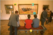
(a) Patch shuffle

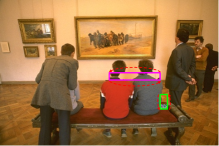
(b) Random shift

Figure 3: The illustrations for our patch jitter augmentation, patch shuffle and random shift. Color frames indicate the changed regions.

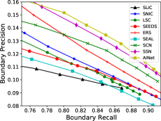
(a) BR-BP on BSDS500

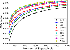
(b) ASA on BSDS500

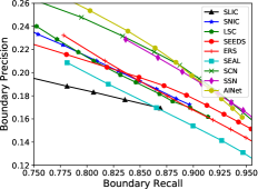
(c) BR-BP on NYUv2

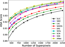
(d) ASA on NYUv2

Figure 4: Performance comparison on datasets BSDS500 and NYUv2.

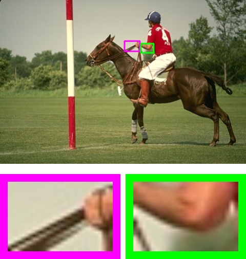
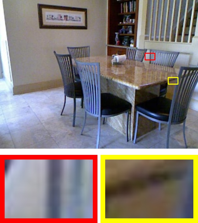
(a) Inputs

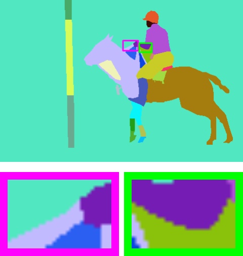
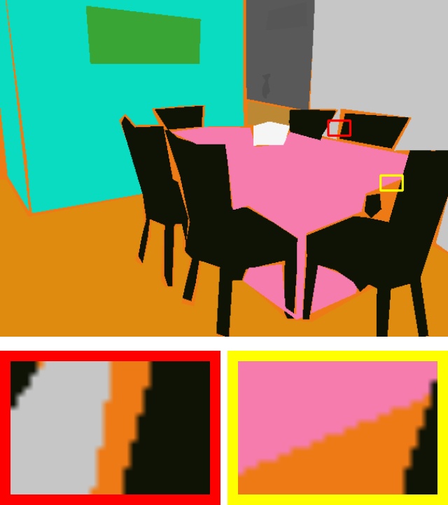
(b) GT label

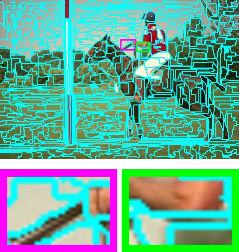
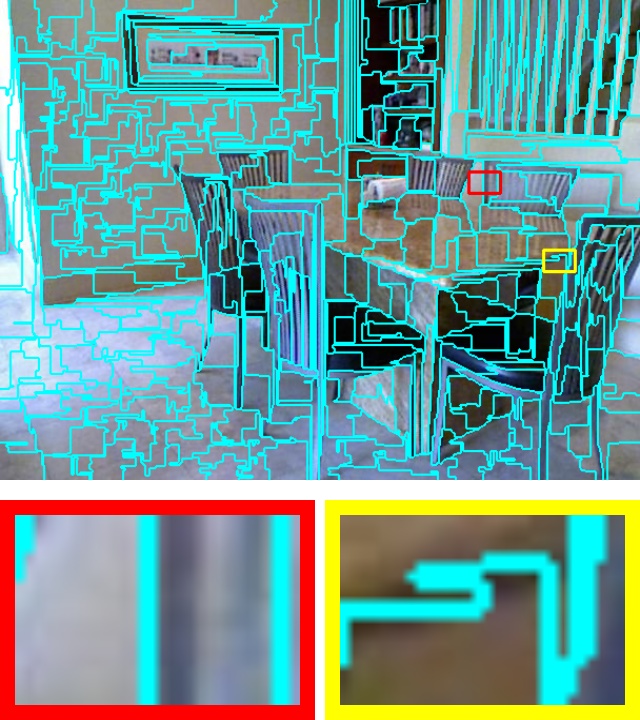
(c) SEAL [37]

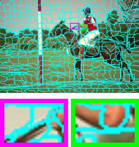
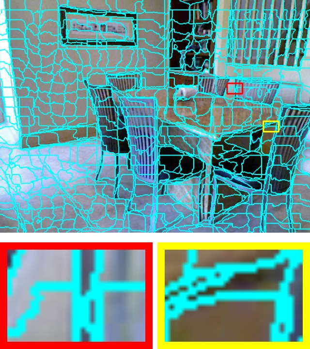
(d) SCN [41]

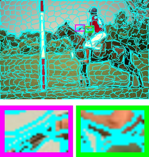
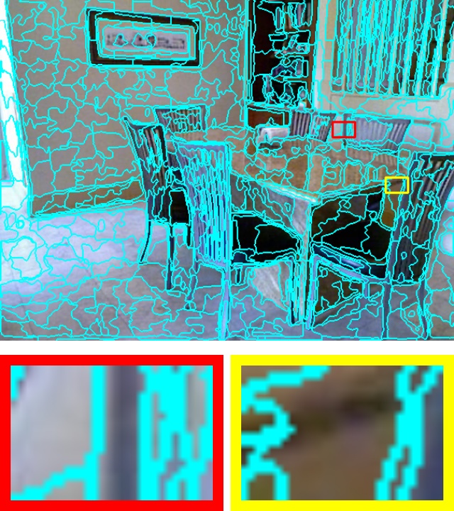
(e) SSN [15]

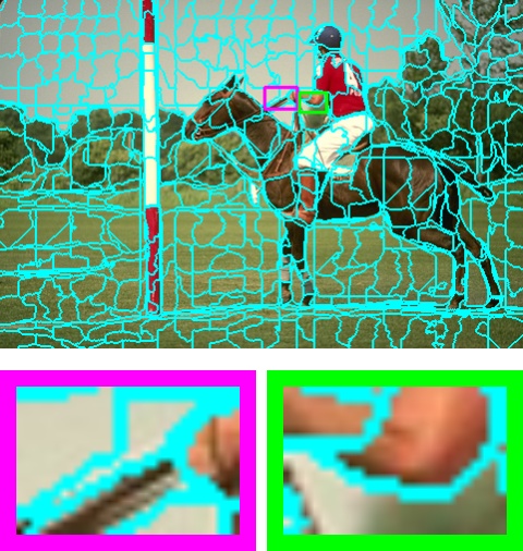
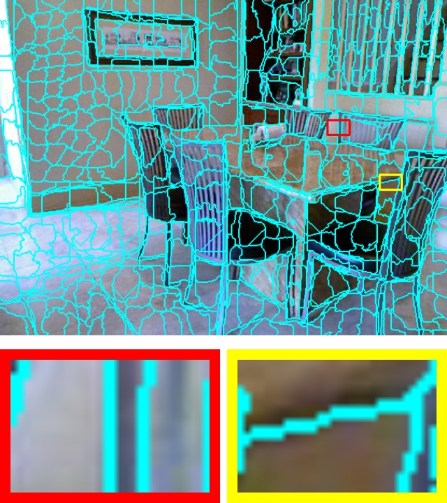
(f) AINet

Figure 5: Qualitative results of four SOTA superpixel methods, SEAL, SCN, SSN, and our AINet. The top row exhibits the results from BSDS500 dataset, while the bottom row shows the superpixels on NYUv2 dataset.

Augmentation via Patch Jitter. To further improve the performance and enhance the generality of our model, we propose to augment the data by jittering the image patches. Specifically, the proposed patch jitter augmentation comprises two components, , patch shuffle and random shift. Fig. 3 shows the respective examples for these two types of data augmentation. The patch shuffle first samples two image patches with shape $S\times S$ and then randomly exchange them to extend the image patterns, the corresponding ground-truth patches are also exchanged accordingly to maintain the consistency. To further augment the data, we randomly pick up one of the selected two patches and replace it with a random patch, whose ground-truth is assigned with a new label. While the random shift could be conducted along with the horizontal or vertical directions. For horizontal random shift, we first randomly sample a patch with shape $S\times L$, where $L=\text{rand\_int}(S,W)$, and a random offset $o=\text{rand\_int}(0,S)$. Then, we conduct a cycle translation on the patch by $o$ offset towards left or right. Meanwhile, the random patch trick in patch shuffle could also be adopted. Finally, the augmentation is done by replacing the original patch with the new one. Analogously, the augmentation along vertical direction could be done similarly.

Implementation Details. In training stage, the image is randomly cropped to 208$\times$208 as input, and the network is trained using the adam optimizer [17] for 4k iterations with batch size 16. The learning rate starts with 8e-5 and is discounted by 0.5 for every 2K iterations. The sampling interval is fixed as 16, consequently, the encoder part employs 4 convolution&pooling operations to get the superpixel embedding with shape $13\times 13\times 256$. The following decoder module produces the pixel embedding with shape $208\times 208\times 16$ using 4 convolution&deconvolution operations. Then, the channels of superpixel embedding are first compressed by two convolution layers: 256$\Rightarrow$64$\Rightarrow$16, then our AI module is performed. The boundary-perceiving loss also acts on the pixel embedding, where the patch size is set to 5, , $K=5$. In the following, two convolution layers are stacked to predict the association map $Q$ with shape $208\times 208\times 9$. In our practice, simultaneously equipping the boundary-perceiving loss and AI Module could not make the performance step further, therefore, we first train the network using the first two items in Eq. 10 for 3K iterations, and use the boundary-perceiving loss to finetune 1K. Following Yang’s practice  [41], the weight of position reconstruction loss is set to 0.003/16, while the weight for our boundary-perceiving loss is fixed to 0.5, , $\lambda=0.003/16,\alpha=0.5$. In testing, we employ the same strategy as [41] to produce varying numbers of superpixels.

Several methods are considered for performance comparison, including classic methods, SLIC [1], LSC [20], ERS [22], SEEDS [6], SNIC [2] and deep learning-based methods, SEAL [37], SSN [15], SCN [41]. We simply use the OpenCV implementation for methods SLIC, LSC and SEEDS. For other methods, we use the official implementations with the recommended parameters from the authors.

Evaluation Metrics. We use three popular metrics including achievable segmentation accuracy (ASA), boundary recall (BR) and boundary precision (BP) to evaluate the performance of superpixel. ASA score studies the upper bound on the achievable segmentation accuracy using superpixel as pre-processing step, while BR and BP focus on accessing how well the superpixel model could identify the semantic boundaries. The higher value of these metrics indicates better superpixel segmentation performance. More detailed description and analysis for these three metrics could be found in [33].

5.1 Comparison with the state-of-the-arts

Fig. 4 reports the quantitative comparison results on BSDS500 and NYUv2 test sets. As indicated in Fig. 4, our AINet attains the best ASA score and BR-BP on both datasets. With the help of deep convolution networks, the methods, SEAL, SCN, SSN, and AINet could achieve superior or comparable performance against the traditional superpixel algorithms, and our AINet is the best model among them. From Fig. 4 (a)-(b), the AINet could surpass the traditional methods by a large margin on BSDS500 dataset. By harvesting the pixel-sueprpixel level context and highlighting the boundaries, AINet could also outperform the deep methods SEAL, SCN and SSN. Fig. 4 (c)-(d) shows the performance when adapting to the NYUv2 test set, we can observe that the AINet also shows better generality. Although the BR-BP is comparable with the SCN and SSN, our ASA score is more outstanding than all of the competitive methods.

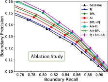
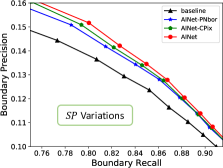
Figure 6: Ablation study on BSDS500. The left figure shows the contributions of each component in our system, while the right one discusses two variations of $SP$ (Eq. 4).

(a) Images

(b) SEAL [37]

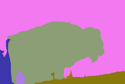
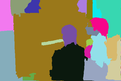
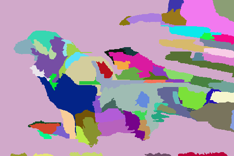
(c) SCN [41]

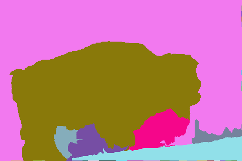
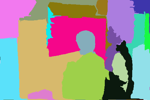
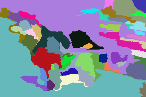
(d) SSN [15]

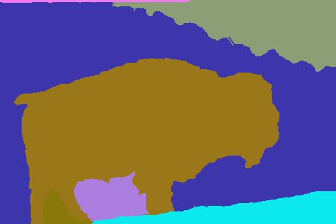
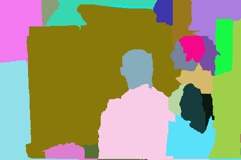
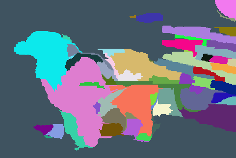
(e) AINet

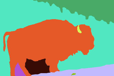
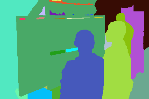
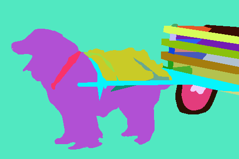
(f) GT label

I: The generated proposals from DEL [23] using different superpixels.

(a) Images

(b) Threshold=0.3

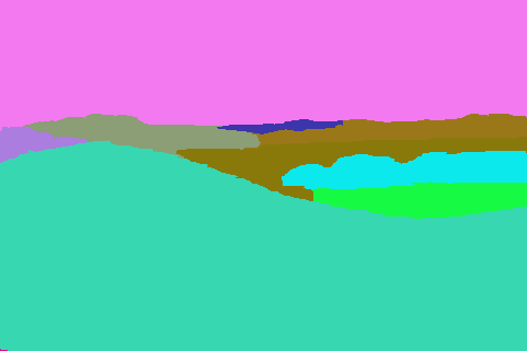
(c) Threshold=0.4

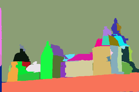
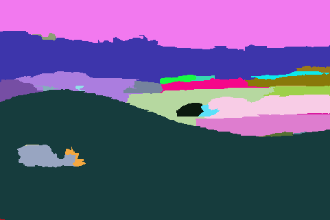
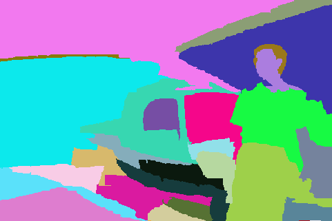
(d) Threshold=0.5

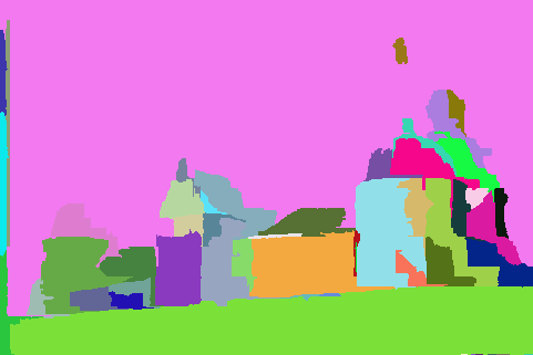
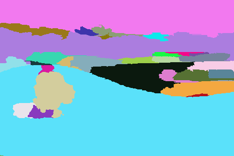
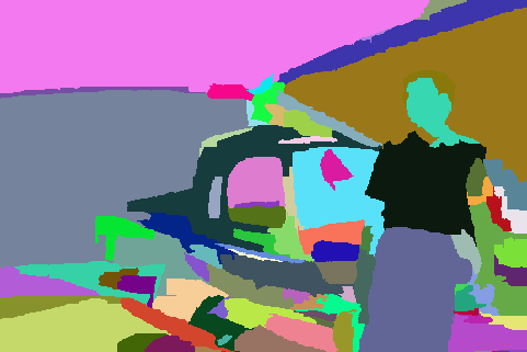
(e) Threshold=0.6

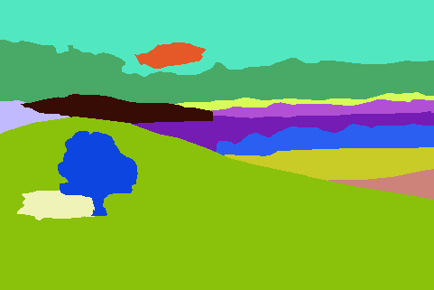
(f) GT label

II: The generated proposals using different thresholds (1 as upper bound).

Figure 7: Qualitative proposals from DEL [23] using different superpixels (I), and the results of DEL [23] with our superpixel using different thresholds (II), where threshold=0.3 mean merging the adjacent superpixels if their similarity is above 0.3.

Fig. 5 shows the qualitative results of four state-of-the-art methods on dataset BSDS500 and NYUv2, comparing to the competing methods, the boundaries of our results are more accurate and clearer, which intuitively shows the superiority of our method.

5.2 Ablation Study

To validate the respective contributions of our proposed modules including the data augmentation trick, AI module, and the boundary-perceiving loss, we conduct ablation study on BSDS500 dataset to thoroughly study their effectiveness. The left figure in Fig. 6 reports the performances of all methods, where the BPL means the boundary-perceiving loss, and BPL+PJ stands for the baseline simultaneously equipped with the boundary-perceiving loss and the patch jitter augmentation. From Fig. 6, we can observe that individually applying the three modules on the baseline method could all boost the performance, and the boundary-perceiving loss could contribute the most performance gains. The combination of the patch jitter augmentation and the BPL or AI Module could make the performance step further, and the AI module equipped with the data augmentation achieves better performance. When simultaneously employing the three modules, we could harvest the best BR-BP.

Besides, we also give a discussion for two alternative choices of $SP$ (Eq. 4): a greedy version of $SP$ that further adds the neighbor pixels to the corresponding surrounding superpixels like the central position, for example, $\hat{m}_{t}$ is replaced by $\hat{m}_{t}+e_{t}$; And a simplified version that ignoring the central superpixel, , $\hat{m}_{c}+e_{p}$ changes to $e_{p}$. The models with the above two versions of $SP$ are marked as AINet-PNbor and AINet-CPix, respectively. The right figure of Fig. 6 shows the results, we can observe that AINet-PNbor and AINet-CPix could both surpass the baseline but perform a litter worse than AINet. By summing the neighbor pixels, the AINet-PNbor could integrate the pixel-wise relation, on the other hand, the sum operation would also reduce the force of superpixel embedding, which would conspire against capturing the pixel-superpixel context. For AINet-CPix, the excluded $\hat{m}_{c}$ is also one of the neighbor superpixels, directly abandoning $\hat{m}_{c}$ would fail to explicitly perceive the relation between pixel $e_{p}$ and central superpixel $\hat{m}_{c}$. Consequently, the above two variations of $SP$ are both not effective to capture the super context.

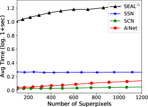
Figure 8: The average time costs of four deep learning based methods w.r.t number of superpixels. The runtime is added with 1 and scaled by logarithmic to show positive values and a clear tendency.

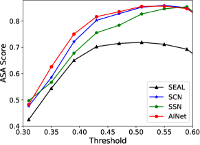
Figure 9: The ASA scores of four state-of-the-art methods on object proposal generation.

5.3 Inference Efficiency

Besides the performance, the inference speed is also a concerned aspect. Therefore, we conduct experiments on BSDS500 dataset to investigate the inference efficiency of four deep learning-based methods. To make a fair comparison, we only count the time of network inference and post-processing steps (if available). All methods run on the same workstation with NVIDIA 1080Ti GPU and Intel E5 CPU.

The time costs of four deep learning-based methods, SEAL, SCN, SSN and our AINet are reported in Fig. 8. The method SCN achieves the best inference efficiency due to its simple architecture, while our AINet introduces more layers and operations, consequently, the inference is slightly slower than the SCN. The superpixel segmentation of SEAL and SSN is much complex comparing to the SCN and our AINet, SEAL needs first output the learned deep features and then feed them to a traditional algorithm to conduct superpixel segmentation, and SSN further performs the $K$-means iteration after obtaining the pixel affinity. As a result, SEAL and SSN both cost much more time in inference stage. Although the SCN is faster, the performance of AINet is much better than SCN. Comparing to these competing methods, our AINet achieves a good trade-off between the performance and the inference efficiency.

5.4 Application on Object Proposal Generation

Image annotation is one of the important application scenarios for superpixels, since it could identify the semantic boundaries and provide the outlines of many semantic regions. To generate the object proposals, Liu et al. [23] propose a model named DEL, they first estimate the similarities between superpixels and merge them according to a certain threshold, by which the proposed method could flexibly control the grain size of object proposal. In this subsection, we feed the superpixels from four state-of-the-art methods, SEAL, SCN, SSN and our AINet to the framework of [23] to further investigate the superiority of our AINet. To evaluate the performance, we use the ASA score to measure how well the produced object proposals cover the ground-truth labels:

$$ASA(O,G)=\frac{1}{N}\sum_{O_{k}}\max_{G_{k}}{\{|O_{k}\cap G_{k}|\}},$$ (11)

where $N$ is the number of generated object proposal $O$, and $G$ is the ground-truth semantic label.

The performance of all methods is reported in Fig. 9, from which we can observe that the average performance of our AINet is more outstanding. Fig. 7 I shows three results of DEL [23] with the superpixels from four methods, different thresholds are used to produce varied size proposals: the adjacent superpixels would be merged if their similarity is above the threshold, which means that higher value would produce finer object proposals. As shown in Fig. 7 I, our AINet could generate more satisfactory object proposals comparing to the competing methods, which validates the effectiveness of our proposed method. Fig. 7 II exhibits the results using the superpixels of our AINet with different thresholds, varying sizes of generated object proposals could be generated by adjusting the threshold.

6 Conclusion

We have presented an association implantation network for superpixel segmentation task. A novel association implantation module is proposed to provide the consistent pixel-superpixel level context for superpixel segmentation task. To pursue better boundary precision, a boundary-perceiving loss is designed to improve the discrimination of pixels around boundaries in hidden feature level, and a data augmentation named patch jitter is developed to further improve the performance. Experiments on two popular benchmarks show that the proposed method could achieve state-of-the-art performance with good generalizability. What’s more, the produced superpixels by our method could also perform well when applied to the object proposal generation. In the future, we will continue to study the effectiveness of the proposed AINet on the stereo matching task.

References

- [1] Radhakrishna Achanta, Appu Shaji, Kevin Smith, Aurélien Lucchi, Pascal Fua, and Sabine Süsstrunk. SLIC superpixels compared to state-of-the-art superpixel methods. IEEE Trans. Pattern Anal. Mach. Intell.(TPAMI), 34(11):2274–2282, 2012.
- [2] Radhakrishna Achanta and Sabine Süsstrunk. Superpixels and polygons using simple non-iterative clustering. In IEEE Conference on Computer Vision and Pattern Recognition (CVPR), pages 4895–4904, June 2017.
- [3] Pablo Arbelaez, Michael Maire, Charless C. Fowlkes, and Jitendra Malik. Contour detection and hierarchical image segmentation. IEEE Trans. Pattern Anal. Mach. Intell., 33(5):898–916, 2011.
- [4] András Bódis-Szomorú, Hayko Riemenschneider, and Luc Van Gool. Superpixel meshes for fast edge-preserving surface reconstruction. In IEEE Conference on Computer Vision and Pattern Recognition (CVPR), pages 2011–2020, June 2015.
- [5] Dorin Comaniciu and Peter Meer. Mean shift: A robust approach toward feature space analysis. IEEE Trans. Pattern Anal. Mach. Intell., 24(5):603–619, 2002.
- [6] Michael Van den Bergh, Xavier Boix, Gemma Roig, and Luc Van Gool. SEEDS: superpixels extracted via energy-driven sampling. Int. J. Comput. Vis. (IJCV), 111(3):298–314, 2015.
- [7] Xiaoyi Dong, Jiangfan Han, Dongdong Chen, Jiayang Liu, Huanyu Bian, Zehua Ma, Hongsheng Li, Xiaogang Wang, Weiming Zhang, and Nenghai Yu. Robust superpixel-guided attentional adversarial attack. In IEEE Conference on Computer Vision and Pattern Recognition (CVPR), pages 12892–12901, June 2020.
- [8] Pedro F. Felzenszwalb and Daniel P. Huttenlocher. Efficient graph-based image segmentation. Int. J. Comput. Vis.(IJCV), 59(2):167–181, 2004.
- [9] Raghudeep Gadde, Varun Jampani, Martin Kiefel, Daniel Kappler, and Peter V. Gehler. Superpixel convolutional networks using bilateral inceptions. In European Conference on Computer Version (ECCV), pages 597–613, Oct. 2016.
- [10] Utkarsh Gaur and B. S. Manjunath. Superpixel embedding network. IEEE Trans. Image Process., 29:3199–3212, 2020.
- [11] Shengfeng He, Rynson W. H. Lau, Wenxi Liu, Zhe Huang, and Qingxiong Yang. Supercnn: A superpixelwise convolutional neural network for salient object detection. Int. J. Comput. Vis., 115(3):330–344, 2015.
- [12] Shengfeng He, Rynson W. H. Lau, Wenxi Liu, Zhe Huang, and Qingxiong Yang. Supercnn: A superpixelwise convolutional neural network for salient object detection. Int. J. Comput. Vis. (IJCV), 115(3):330–344, 2015.
- [13] Shengfeng He, Rynson W. H. Lau, Wenxi Liu, Zhe Huang, and Qingxiong Yang. Supercnn: A superpixelwise convolutional neural network for salient object detection. Int. J. Comput. Vis.(IJCV), 115(3):330–344, 2015.
- [14] Yinlin Hu, Rui Song, Yunsong Li, Peng Rao, and Yangli Wang. Highly accurate optical flow estimation on superpixel tree. Image Vis. Comput., 52:167–177, 2016.
- [15] Varun Jampani, Deqing Sun, Ming-Yu Liu, Ming-Hsuan Yang, and Jan Kautz. Superpixel sampling networks. In European Conference on Computer Vision (ECCV), pages 363–380, Sep. 2018.
- [16] Xuejing Kang, Lei Zhu, and Anlong Ming. Dynamic random walk for superpixel segmentation. IEEE Trans. Image Process., 29:3871–3884, 2020.
- [17] Diederik P. Kingma and Jimmy Ba. Adam: A method for stochastic optimization. In International Conference on Learning Representations (ICLR), May 2015.
- [18] Suha Kwak, Seunghoon Hong, and Bohyung Han. Weakly supervised semantic segmentation using superpixel pooling network. In Proceedings of the Thirty-First AAAI Conference on Artificial Intelligence,, pages 4111–4117, Feb. 2017.
- [19] Alex Levinshtein, Adrian Stere, Kiriakos N. Kutulakos, David J. Fleet, Sven J. Dickinson, and Kaleem Siddiqi. Turbopixels: Fast superpixels using geometric flows. IEEE Trans. Pattern Anal. Mach. Intell., 31(12):2290–2297, 2009.
- [20] Zhengqin Li and Jiansheng Chen. Superpixel segmentation using linear spectral clustering. In IEEE Conference on Computer Vision and Pattern Recognition (CVPR), pages 1356–1363, 2015.
- [21] Zhenguo Li, Xiao-Ming Wu, and Shih-Fu Chang. Segmentation using superpixels: A bipartite graph partitioning approach. In IEEE Conference on Computer Vision and Pattern Recognition (CVPR), pages 789–796, June 2012.
- [22] Ming-Yu Liu, Oncel Tuzel, Srikumar Ramalingam, and Rama Chellappa. Entropy rate superpixel segmentation. In IEEE Conference on Computer Vision and Pattern Recognition (CVPR), pages 2097–2104, June 2011.
- [23] Yun Liu, Peng-Tao Jiang, Vahan Petrosyan, Shi-Jie Li, Jiawang Bian, Le Zhang, and Ming-Ming Cheng. DEL: deep embedding learning for efficient image segmentation. In Proceedings of the Twenty-Seventh International Joint Conference on Artificial Intelligence (IJCAI), pages 864–870, July 2018.
- [24] Yong-Jin Liu, Cheng-Chi Yu, Minjing Yu, and Ying He. Manifold SLIC: A fast method to compute content-sensitive superpixels. In IEEE Conference on Computer Vision and Pattern Recognition (CVPR), pages 651–659, 2016.
- [25] Jiangbo Lu, Hongsheng Yang, Dongbo Min, and Minh N. Do. Patch match filter: Efficient edge-aware filtering meets randomized search for fast correspondence field estimation. In IEEE Conference on Computer Vision and Pattern Recognition (CVPR), pages 1854–1861, June 2013.
- [26] Vaïa Machairas, Matthieu Faessel, David Cárdenas-Peña, Théodore Chabardès, Thomas Walter, and Etienne Decencière. Waterpixels. IEEE Trans. Image Process., 24(11):3707–3716, 2015.
- [27] Cheng Ouyang, Carlo Biffi, Chen Chen, Turkay Kart, Huaqi Qiu, and Daniel Rueckert. Self-supervision with superpixels: Training few-shot medical image segmentation without annotation. In European Conference on Computer Version (ECCV), pages 762–780, Aug. 2020.
- [28] Xiaofeng Ren and Jitendra Malik. Learning a classification model for segmentation. In IEEE International Conference on Computer Vision (ICCV), pages 10–17, Oct. 2003.
- [29] Olaf Ronneberger, Philipp Fischer, and Thomas Brox. U-net: Convolutional networks for biomedical image segmentation. In Medical Image Computing and Computer-Assisted Intervention (MICCAI), pages 234–241, Oct. 2015.
- [30] Abhishek Sharma, Oncel Tuzel, and Ming-Yu Liu. Recursive context propagation network for semantic scene labeling. In Advances in Neural Information Processing Systems (NIPS), pages 2447–2455, Dec. 2014.
- [31] Evan Shelhamer, Jonathan Long, and Trevor Darrell. Fully convolutional networks for semantic segmentation. IEEE Trans. Pattern Anal. Mach. Intell., 39(4):640–651, 2017.
- [32] Nathan Silberman, Derek Hoiem, Pushmeet Kohli, and Rob Fergus. Indoor segmentation and support inference from RGBD images. In European Conference on Computer Version (ECCV), pages 746–760, Oct. 2012.
- [33] David Stutz, Alexander Hermans, and Bastian Leibe. Superpixels: An evaluation of the state-of-the-art. Comput. Vis. Image Underst., 166:1–27, 2018.
- [34] Deqing Sun, Ce Liu, and Hanspeter Pfister. Local layering for joint motion estimation and occlusion detection. In IEEE Conference on Computer Vision and Pattern Recognition (CVPR), pages 1098–1105, June 2014.
- [35] Wen Sun, Qingmin Liao, Jing-Hao Xue, and Fei Zhou. SPSIM: A superpixel-based similarity index for full-reference image quality assessment. IEEE Trans. Image Process., 27(9):4232–4244, 2018.
- [36] Teppei Suzuki, Shuichi Akizuki, Naoki Kato, and Yoshimitsu Aoki. Superpixel convolution for segmentation. In IEEE International Conference on Image Processing (ICIP), pages 3249–3253, Oct 2018.
- [37] Wei-Chih Tu, Ming-Yu Liu, Varun Jampani, Deqing Sun, Shao-Yi Chien, Ming-Hsuan Yang, and Jan Kautz. Learning superpixels with segmentation-aware affinity loss. In IEEE Conference on Computer Vision and Pattern Recognition (CVPR), pages 568–576, June 2018.
- [38] Olga Veksler, Yuri Boykov, and Paria Mehrani. Superpixels and supervoxels in an energy optimization framework. In European Conference on Computer Vision (ECCV), pages 211–224, Sep. 2010.
- [39] Koichiro Yamaguchi, David A. McAllester, and Raquel Urtasun. Robust monocular epipolar flow estimation. In IEEE Conference on Computer Vision and Pattern Recognition (CVPR), pages 1862–1869, June 2013.
- [40] Chuan Yang, Lihe Zhang, Huchuan Lu, Xiang Ruan, and Ming-Hsuan Yang. Saliency detection via graph-based manifold ranking. In IEEE Conference on Computer Vision and Pattern Recognition (CVPR), pages 3166–3173, June 2013.
- [41] Fengting Yang, Qian Sun, Hailin Jin, and Zihan Zhou. Superpixel segmentation with fully convolutional networks. In IEEE Conference on Computer Vision and Pattern Recognition (CVPR), pages 13961–13970, June 2020.
- [42] Donghun Yeo, Jeany Son, Bohyung Han, and Joon Hee Han. Superpixel-based tracking-by-segmentation using markov chains. In IEEE Conference on Computer Vision and Pattern Recognition (CVPR), pages 511–520, June 2017.
- [43] Wangjiang Zhu, Shuang Liang, Yichen Wei, and Jian Sun. Saliency optimization from robust background detection. In IEEE Conference on Computer Vision and Pattern Recognition (CVPR), pages 2814–2821, June 2014.