Probing Multiple Electric Dipole Forbidden Optical Transitions in Highly Charged Nickel Ions

Abstract

Highly charged ions (HCIs) are promising candidates for the next generation of atomic clocks, owing to their tightly bound electron cloud, which significantly suppresses the common environmental disturbances to the quantum oscillator. Here we propose and pursue an experimental strategy that, while focusing on various HCIs of a single atomic element, keeps the number of candidate clock transitions as large as possible. Following this strategy, we identify four adjacent charge states of nickel HCIs that offer as many as six optical transitions. Experimentally, we demonstrated the essential capability of producing these ions in the low-energy compact Shanghai-Wuhan Electron Beam Ion Trap. We measured the wavelengths of four magnetic-dipole ($M$1) and one electric-quadrupole ($E$2) clock transitions with an accuracy of several ppm with a novel calibration method; two of these lines were observed and characterized for the first time in controlled laboratory settings. Compared to the earlier determinations, our measurements improved wavelength accuracy by an order of magnitude. Such measurements are crucial for constraining the range of laser wavelengths for finding the “needle in a haystack” narrow lines. In addition, we calculated frequencies and quality factors, evaluated sensitivity of these six transitions to the hypothetical variation of the electromagnetic fine structure constant $\alpha$ needed for fundamental physics applications. We argue that all the six transitions in nickel HCIs offer intrinsic immunity to all common perturbations of quantum oscillators, and one of them has the projected fractional frequency uncertainty down to the remarkable level of 10^-19.

I INTRODUCTION

Quantum metrology of atomic time-keeping has seen dramatic improvements over the past decade with novel applications spanning from chronometric geodesy [1, 2] to fundamental physics, such as dark matter searches [3, 4] and multi-messenger astronomy [5]. Currently, optical atomic clocks using neutral atoms or singly charged ions have demonstrated fractional frequency uncertainties at the level of $10^{-18}$ or even $10^{-19}$ [6, 7, 8, 9]. These uncertainties refer to the ability to protect the quantum oscillator from environmental perturbations, such as stray magnetic and electric fields. As these existing technologies mature, they are reaching the stage where one needs to understand numerous sources of environmental perturbations in greater detail. In some cases, the perturbations cannot be fully eliminated and one needs to devote significant efforts to measuring and characterizing the perturbations; these lead to non-universal systematic corrections to the clock frequency that are specific to experimental realization of the clock.

Novel classes of atomic clocks must start with quantum oscillators that offer a much more improved inherent immunity to environmental perturbations than the more mature technologies. One of such systems is the nuclear clock based on the unique property of the ²²⁹Th nucleus – the existence of a nuclear transition in a laser-accessible range [10, 11]; unfortunately, despite substantial world-wide efforts [12, 13], this transition is yet to be observed directly. The suppression of environmental perturbations for the nuclear oscillator comes from the nuclear size being $\sim 10^{4}$ times smaller than the size of a neutral atom. Alternative novel systems are highly charged ions (HCIs) [14, 15]. Similar to the nuclear clock, here the oscillator size is also substantially reduced, owing to the electronic cloud size shrinking as $1/Z$ with the increasing ion charge $Z$. HCIs were proposed as promising candidates for the next generation of atomic clocks [14]. In addition, beyond the improved time-keeping, HCIs open intriguing opportunities for probing new physics beyond the standard model of particle physics [16, 17].

Compared to the single, yet to be spectroscopically found nuclear transition, there is a plethora of suitable HCIs (see a review [18] for a sample of proposals). A detailed analysis [19] indicates that with certain HCIs, atomic clocks “can have projected fractional accuracies beyond the $10^{-20}-10^{-21}$ level for all common systematic effects, such as blackbody radiation, Zeeman, ac-Stark, and quadrupolar shifts”. Moreover, compared to the nuclear clock, where the direct observation of the clock transition remains elusive, the clock transitions in HCIs can be found with conventional spectroscopy or from atomic-structure computations. Indeed, here we report spectrographic measurements of wavelengths for five clock transitions with an accuracy of several ppm (see Table 1), setting up the stage for the more accurate laser spectroscopy.

Table 1: Observed and calculated wavelengths of magnetic-dipole ($M$1) and electric-quadrupole ($E$2) transitions, where the lines $a$ through $f$ are candidate clock transitions, in nm.

Line	Ion	Transition	Type	NIST	This work
				Vacuum	Air (observed)	Vacuum	Theory
$a$	Ni11+	$3s^{2}3p^{5}\;\;{}^{2}\!P_{1/2}-{{}^{2}\!P}_{3/2}$	$M$1	423.2	423.104(2)	423.223(2)	423.0(6)
$b$	Ni12+	$3s^{2}3p^{4}\;\;{}^{3}\!P_{1}-{{}^{3}\!P}_{2}$	$M$1	511.724	511.570(2)	511.713(2)	511.8(6)
$c$	Ni14+	$3s^{2}3p^{2}\;\;{}^{3}\!P_{1}-{{}^{3}\!P}_{0}$	$M$1	670.36	670.167(2)	670.352(2)	671.1(14)
$d$	Ni15+	$3s^{2}3p\;\;^{2}\!P_{3/2}-{{}^{2}\!P}_{1/2}$	$M$1	360.22	360.105(2)	360.207(2)	359.9(9)
$e$	Ni12+	$3s^{2}3p^{4}\;\;{}^{3}\!P_{0}-{{}^{3}\!P}_{2}$	$E$2	498.50(249)	–	–	496.9(24)
$f$	Ni14+	$3s^{2}3p^{2}\;\;{}^{3}\!P_{2}-{{}^{3}\!P}_{0}$	$E$2	365.277	–	365.278(1)	365.0(3)
$g$	Ni14+	$3s^{2}3p^{2}\;\;{}^{3}\!P_{2}-{{}^{3}\!P}_{1}$	$M$1	802.63	802.419(2)	802.639(2)	800.3(25)

Despite the lack of suitable electric-dipole ($E$1) transitions for direct laser cooling, recent successes in sympathetic cooling and quantum logic spectroscopy of HCIs have paved way for precision spectroscopic measurements with HCIs [20, 21]. It is worth emphasizing that these newly demonstrated technologies can be applied universally to a wide range of HCIs. The multitude of suitable clock HCI candidates is a “blessing in disguise”, as one needs to commit to building the infrastructure for a specific ion. As with any new endeavor, one would like to mitigate potential problems with picking a “wrong” ion. Here we propose and pursue a straddling strategy that would allow one to explore several clock transitions using not only the same HCI production system but also ions of the same atomic element.

A suitable HCI has to possess a number of properties enabling precision spectroscopy and compatibility with operating an atomic clock. Generally, one may distinguish between three classes of visible or near visible optical forbidden transitions in HCIs that can be used for developing optical clocks:

1. Magnetic-dipole ($M$1) transitions between two hyperfine-structure levels of the same electronic state [22, 19].

2. Forbidden transitions between level crossing electronic states, which tend to be sensitive to variation of the fine structure constant [16, 23, 24, 25].

3. Forbidden transitions between the ground-state fine structure levels [14, 19, 26, 27].

Type 1 transitions occur in few-electron heavy HCIs [19] that are challenging to produce and trap. Type 2 transitions involve a complex energy structure that can impede initialization and read-out of the clock states. Here we focus on type 3 transitions that offer simplicity in both producing the ions and clock operation. More specifically we choose HCIs of nickel of various charge states [19, 26, 27]: Ni¹¹⁺, Ni¹²⁺, Ni¹⁴⁺, and Ni¹⁵⁺. The clock transitions are shown in Fig. 1. All the traditional clock perturbations are strongly suppressed for these ions due to the charge scaling arguments [28, 14, 19]. As pointed out in Ref. [14], the major issue with HCI clocks is the so-called quadrupolar shift of the clock transition, when the quadrupole ($Q$) moment of the clock state couples to the always existing $E$-field gradients in ion traps. While the $Q$-moment of an electronic cloud does scale as $1/Z^{2}$, this reduction is not sufficient to suppress the quadrupolar shift below the desired level of accuracy. Thus, it is beneficial to select clock states with either vanishing or strongly suppressed $Q$-moments.

There are four $M$1 and two $E$2 optical transitions in Ni¹¹⁺, Ni¹²⁺, Ni¹⁴⁺, and Ni¹⁵⁺ that offer the desired flexibility. These ions have varying number of electrons in the $3p$ shell, see Fig. 1. The clock transitions are between the fine structure components of the ground electronic state. There are four stable isotopes ⁵⁸Ni, ⁶⁰Ni, ⁶²Ni, and ⁶⁴Ni without nuclear spin; these can be used to search for new physics with isotope shift measurements [29, 30, 31] and for initial spectroscopic measurements. These spin-0 isotopes, however, will be susceptible to the quadrupolar shifts for clock transitions. However, these shifts can be suppressed by using the ⁶¹Ni isotope (nuclear spin $I=3/2$), which has a natural abundance of 1.14%. Then the quadrupolar shifts can be either strongly suppressed or completely removed by employing the following clock transitions between hyperfine states (see Fig. 1):

• ${{}^{2}\!P}_{3/2}\,F=0$ and ${}^{2}\!P_{1/2}\,F=1$ or $F=2$ for Ni¹¹⁺ and Ni¹⁵⁺,

• ${}^{3}\!P_{1}\,F=1/2$ and ${}^{3}\!P_{2}\,F=1/2$ for Ni¹²⁺,

• ${}^{3}\!P_{1}\,F=1/2$ and ${}^{3}\!P_{0}\,F=3/2$ for Ni¹⁴⁺,

• ${}^{3}\!P_{0}\,F=3/2$ and ${}^{3}\!P_{2}\,F=1/2$ for Ni¹²⁺ and Ni¹⁴⁺.

This selection is based on the following reasoning [19]: $Q$-moments (rank 2 tensors) of the $F=0$ and $F=1/2$ states are zero due to selection rules. For the ${}^{2}\!P_{1/2}\,F=1,2$ and ${}^{3}\!P_{0}\,F=3/2$ states, the electronic $Q$-moments vanish due to selection rules for the electronic angular momentum $J$. Thereby, the $Q$-moments are determined by the nuclear $Q$-moments or hyperfine mixing [11] and, as such, are strongly suppressed. As an indication of attainable accuracy, Refs. [26, 27] evaluated relevant properties of the clock transitions in ⁶¹Ni¹⁵⁺ and ⁵⁸Ni¹²⁺ and estimated common systematic uncertainties to be below $10^{-19}$, in line with the more general estimates of Ref. [19]. The second-order Doppler shift induced by the excess micromotion of the trapped ion is expected to be suppressed to below $10^{-19}$ by compensating the stray electric field to a level below 0.1 V/m [32, 33]. In a cryogenic trap, the heating rate of the trapped ions caused by the collisions with the background gas and the anomalous motional heating is reduced, and hence the second-order Doppler shift induced by the secular motion is also expected to be sufficiently small [18]. Based on these arguments, we expect the attainable fractional systematic uncertainty of all the six clock transitions in Ni HCIs to be $10^{-19}$.

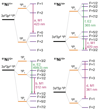
Figure 1: Partial energy-level diagrams for highly charged nickel ions. Clock transitions are explicitly drawn. Magnetic-dipole ($M$1) transitions are shown in magenta and electric-quadrupole ($E$2) transitions in green. The labeling of transitions is the same as in Table 1.

As the first essential step towards realizing the Ni HCI clocks, we produced the target ions at our newly built low-energy compact Shanghai-Wuhan Electron Beam Ion Trap (SW-EBIT) [34]. The wavelengths of four $M$1 and one $E$2 clock transitions between the ground-state fine structure levels in these ions are measured to an accuracy of several ppm using a spectrograph. In particular, the three $M$1 lines $b$, $c$, and $g$ (listed in Table 1) in Ni¹²⁺ and Ni¹⁴⁺ are observed and characterized for the first time in the laboratory. We also carried out calculations for these ions using an ab initio relativistic method of atomic structure, the multi-configuration Dirac-Hartree-Fock (MCDHF) method [35, 36]. We evaluated relevant spectroscopic properties, such as transition wavelengths and natural linewidths. We also estimated the sensitivity to the hypothetical variation of the fine structure constant $\alpha$ and found that all considered clock transitions in Ni HCIs are more susceptible to the variation than most of the commonly employed singly charge ions or neutral atoms. Thus, Ni HCIs can be used for placing stringent constraints on the spatial or temporal variation of $\alpha$.

II EXPERIMENTAL METHOD AND RESULTS

II.1 Production of Ni HCIs

To produce Ni HCIs, we injected the Ni(C₅H₅)₂ (nickelocene) molecular beam into the trap center. Then the charge-state distribution of Ni HCIs was measured using the electron-beam current of 6 mA and the electron-beam energy of 500 eV, which is higher than the ionization energies 319.5 eV, 351.6 eV, 429.3 eV, and 462.8 eV needed for Ni¹¹⁺, Ni¹²⁺, Ni¹⁴⁺, and Ni¹⁵⁺, respectively. The extraction period was 0.3 s and the magnetic flux density was 0.16 T. As shown in Fig. 2, the target ions Ni¹¹⁺, Ni¹²⁺, Ni¹⁴⁺, and Ni¹⁵⁺ were produced, and the ions of two distinct isotopes, ⁶⁰Ni and ⁵⁸Ni, were resolved. The techniques for measuring charge-state distribution are described in Ref. [34].

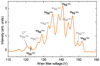
Figure 2: Charge-state distribution of the Ni HCIs, obtained by averaging 3 measurements.

II.2 Spectral measurements

The spectra of the trapped Ni HCIs were observed by a Czerny-Turner spectrograph (Andor Kymera 328i) equipped with an Electron Multiplying Charge-Coupled Device (EMCCD, Andor Newton 970, pixel: $1600\times 200$, pixel size: 16 $\mu$m) and a 1200 l/mm grating blazed at 500 nm. To maximize the number of the Ni HCIs of a specific charge state, different electron-beam energies were used, i.e. 370 eV, 400 eV, 500 eV, and 540 eV for Ni¹¹⁺, Ni¹²⁺, Ni¹⁴⁺, and Ni¹⁵⁺, respectively. As illustrated in Fig. 3, the fluorescence emitted from the Ni HCIs was focused by a single N-BK7 Bi-Convex lens (focal length $f=10$ cm at 633 nm) on the spectrograph entrance slit. The distance between the trap (DT2, drift tube 2 in SW-EBIT [34]) center and the front principal plane of the lens remained fixed at 197 mm, which was about twice the focal length. Before setting up the spectrograph, a Charge-Coupled Device (CCD) was placed on the image plane to image the two inner edges of DT2 (1 mm slit width) that were illuminated by the hot cathode. In order to ensure that the lens was aligned with the optical axis, we adjusted the angle and position of the lens until the edge image became mirror-symmetric. Because of the dispersion of the lens, to ensure that the spectrograph slit was always precisely located on the image plane, the distance $L$ between the slit of the spectrograph and the back principal plane of the lens was calculated and adjusted for every central wavelength of the measured spectra. The grating was set to zero-order to image the inner edges of DT2 through spectrograph with its maximum slit width and minimum iris aperture behind the slit. Similarly, the angle and position of the spectrograph were adjusted until the image of the edges became mirror-symmetric to ensure the spectrograph alignment with the optical axis. A one inch aperture was placed before the lens to block the stray light. For calibration, a conjugated optical system was installed on the opposite side of the spectrograph. A diffuser attached by a 0.5 mm slit was placed on the object plane. A low-pressure gas-discharge lamp filled with Kr illuminated the slit, and the slit was imaged to the trap center to overlap with the trapped ion cloud. During the spectral exposure time of 10 to 60 minutes, the Kr lamp as the calibration light source flashed at a period of 1 to 3 minutes. The slit of the spectrograph was set to 30 $\mu$m, and the iris aperture in the spectrograph was set to 40 steps to obtain the F/7.6 aperture. The focal length of the spectrograph was tuned to minimize the linewidth in each spectral range.

All the spectra were binned to a non-dispersive direction after removing the cosmic ray noise, as shown in Fig. 4 (a). The dispersion function was obtained by fitting the NIST-tabulated Ritz in-the-air wavelengths of the calibration lines to a cubic polynomial, against their column numbers of the line centroids. The residuals of the calibration lines and the 1-$\sigma$ fitting confidence band are shown in Fig. 4 (b). To determine the line centroids, the measured lines and calibration lines were fitted to a Gaussian or a multi-Gaussian profile, as shown in Fig. 4 (c).

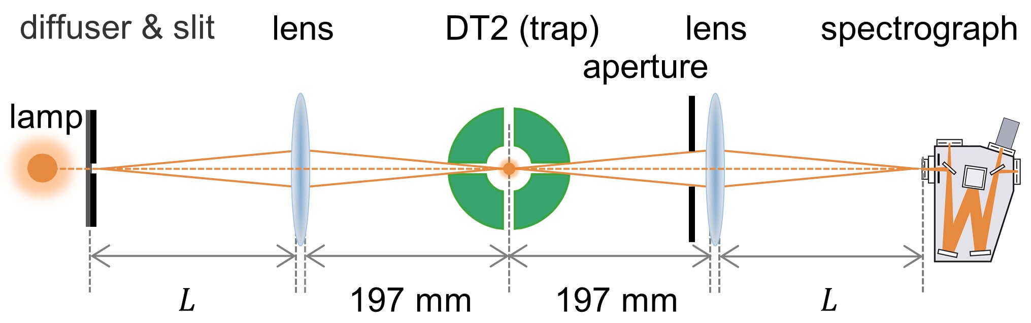
Figure 3: Scheme of observation and calibration of the measured lines. The Ni HCIs are trapped at the center of DT2 in SW-EBIT.

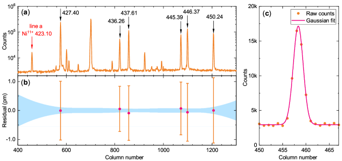
Figure 4: (a) A spectrum of line $a$ from Ni¹¹⁺ and its calibration lines from Kr atom whose approximate wavelengths are labeled in the figure in nm. (b) Residuals of cubic polynomial fits of the calibration lines. The gray band is a 1-$\sigma$ confidence band. The uncertainties in the calibration lines are dominated by the line centroid uncertainties of the Gaussian fits. (c) Spectrum of line $a$ and its Gaussian fit.

II.3 Observed wavelengths

Previously, these five $M$1 lines in Table 1 were observed in the solar corona emission [37] with a wavelength uncertainty of tens of picometer. The lines $a$ and $d$ have been also measured in Tokamak [38, 39], but experimental observation of the other three lines $b$, $c$, and $g$ has not been reported in the literature. In this work, we observed and identified all five $M$1 lines emitted from the nickel plasma in the SW-EBIT in a controlled laboratory setting. The measured wavelengths agree with the Ritz wavelengths in NIST database [40], as shown in Table 1, where the wavelengths between air and vacuum were converted by an empirical equation [41]. However, for line $d$, our result of 360.105(2) nm substantially deviates from the value of 360.123(2) nm observed from Tokamak plasma by Hinnov et al. [39]. To test our result, two lines from Ar⁺ were measured without any change of the optical system comparing to the measurement of line $d$, and the measured wavelengths in air were 357.660(2) nm and 358.843(2) nm, which were in good agreement with the Ritz wavelengths in NIST database, i.e., 357.661538 nm and 358.844021 nm. For the $E$2 lines $e$ and $f$, the transition rates are too small to be observable by our technique. However, we deduced the wavelength of line $f$ in Table 1 from those of lines $c$ and $g$ via the Rydberg-Ritz combination principle.

II.4 Measurement uncertainties

Line centroid uncertainty. The line centroids of the measured lines and their calibration lines were determined by the centers of the fitted Gaussian profiles. Since the statistical uncertainty of the line centroid was mainly caused by the low signal-to-noise ratio, we evaluated the statistical uncertainty by performing at least 20 measurements on the line of interest, as shown in Fig 5. For all five measured lines, this uncertainty was smaller than 0.4 pm. The systematic uncertainty of the line centroid is mainly caused by the non-ideal Gaussianity of the line because of the optical aberration and the Zeeman components. In this work, since the measured lines and their calibration lines shared a similar profile, the optical aberration effect was largely offset. In the trap center, the magnetic flux density was $\sim$0.16 T, resulting in a $\sim$2 pm splitting between the Zeeman components of the clock transitions, which was relatively small (unresolved) compared to the $\sim$90 pm linewidth. Furthermore, the Zeeman effect would not alter the line centroid because the Zeeman components were symmetrically distributed; in addition, the Zeeman effect was negligible for the Kr lamp due to the low magnetic field of 0.4 mT.

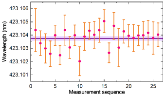
Figure 5: The calibrated wavelengths of line $a$ in air derived from a series of 26 measurements. The wavelength uncertainty of each single spectrum was calculated as the quadrature of the line centroid uncertainty and the 1-$\sigma$ confidence interval of the fitted dispersion function. The weighted average wavelength is represented by the solid purple line and its uncertainty is represented by lilac band.

Dispersion function uncertainty. The statistical uncertainty for the dispersion function was caused by the centroid statistical uncertainties of calibration lines, which were reduced by the statistics of the line centroids. The systematic dispersion function uncertainty of a measured line was estimated by averaging the absolute values of the fitted residuals of its calibration lines of all the measured spectra.

Calibration systematic uncertainty. Since the image of the calibration light source might not be overlapped exactly with the trapped ion cloud, the spatial deviation and misalignment could cause wavelength offset between the measured lines and their calibration lines. In this work, a spatial deviation of less than 2 mm would result in a wavelength uncertainty of less than 1 pm. The misalignment could cause a wavelength uncertainty of less than 1 pm, which was estimated from five measurements of the Ar⁹⁺ 553 nm line by resetting the optical system every time. Thereby, the overall systematic uncertainty caused by our calibration scheme was expected to be less than 2 pm.

Other uncertainties. In this work, the calibration light source and the fluorescence of the trapped ions were exposed to the spectrograph almost simultaneously, indicating that the temperature drift and the mechanical drift were canceled out. The shifts due to the Stark effect and collisions can also be neglected at this level of accuracy. The wavelengths of the selected calibration lines are reliable because their uncertainties in the NIST database are all less than 0.3 pm.

Table 2 is the uncertainty budget for the lines $a$-$d$ and $g$ in air. The total uncertainty was calculated as the quadrature of all the uncertainties, which was dominated by the calibration systematic uncertainty. In order to test the reliability of the uncertainty estimation, the wavelengths in-the-air of the three lines from Ar HCI were measured, i.e., Ar⁹⁺ 553.327(2) nm, Ar¹⁰⁺ 691.689(2) nm, and Ar¹³⁺ 441.255(2) nm, which were consistent with the previous measured values of 553.3265(2) nm, 691.6878(12) nm, and 441.255919(6) nm, respectively [42, 43].

The total wavelength uncertainty of this observation and calibration scheme was approximately 2 pm, which was comparable to the uncertainty of the scheme that the measured lines were calibrated by the lines from the buffer gas observed by a similar resolution spectrograph [44, 45], but larger than the uncertainty of the scheme that the calibration source was overlapped with the real image of the ion cloud observed by a higher resolution spectrograph [42]. Compared to these two schemes, our scheme is more convenient and flexible. The uncertainty may be reduced by using a higher resolution spectrograph that is less sensitive to the calibration optical system.

Table 2: Uncertainty budget of the measured lines.

Source	Uncertainty in wavelength (pm)
Line	$a$	$b$	$c$	$d$	$g$
Line centroid	0.2	0.2	0.1	0.2	0.3
Dispersion function	0.1	0.3	0.3	0.2	0.4
Calibration systematic	2	2	2	2	2
Total	2	2	2	2	2

III THEORETICAL METHOD AND RESULTS

III.1 MCDHF calculations

In the MCDHF method, an atomic wave function $\Psi$ is constructed as a linear combination of configuration state functions (CSFs) $\Phi$ of the same parity $P$, the total angular momentum $J$, and its projection $M_{J}$, i.e.,

$$\Psi(\Gamma PJM_{J})=\sum_{i=1}^{N_{\mathrm{CSF}}}{c_{i}\Phi(\gamma_{i}PJM_{J})}.$$ (1)

Here $c_{i}$ is the mixing coefficient and $\gamma_{i}$ stands for the remaining quantum numbers of the CSFs. Each CSF itself is a linear combination of products of one-electron Dirac orbitals. Both mixing coefficients and orbitals are optimized in the self-consistent field calculation. After a set of orbitals is obtained, the relativistic configuration interaction (RCI) calculations are used to capture more electron correlations. In addition to the Coulomb interactions, our RCI calculations also include the Breit interaction in the low-frequency approximation and the quantum electrodynamic (QED) corrections.

In order to obtain high-quality atomic wave functions, we designed an elaborate computational model as follows. In the first step, the self-consistent field (SCF) calculations were performed successively to generate virtual orbitals. The virtual orbitals were employed to form CSFs which account for certain electron correlations. More specifically, CSFs were produced through single (S)- and double (D)-electron excitations from the occupied Dirac-Hartree-Fock orbitals to virtual orbitals, but the double excitation from the atomic core $1s^{2}2s^{2}2p^{6}$ orbitals were excluded at this stage. The virtual orbitals were augmented layer by layer up to $n_{\rm{max}}=12$ and $l_{\rm{max}}=6$, where $n_{\rm{max}}$ and $l_{\rm{max}}$ denote, respectively, the maximum principal quantum number and the maximum angular quantum number of the virtual orbitals. In the second step, the single-reference configuration RCI calculations were performed with the configuration space constructed from SD excitation from all occupied orbitals to the set of virtual orbitals. In other words, the correlation between electrons in the atomic core, which were neglected in the first step, were captured. In the last step, we considered part of contributions from the triple- and quadruple-excitation CSFs. In order to limit the number of CSFs, the MR-SD approach was adopted to produce corresponding CSFs [46, 47]. The multi-reference (MR) configuration sets were created as $\{3s3p^{5}3d$, $3s^{2}3p^{3}3d^{2}\}$ for Ni¹¹⁺, $\{3s3p^{4}3d$, $3s^{2}3p^{2}3d^{2}$, $3p^{6}\}$ for Ni¹²⁺, $\{3s3p^{2}3d$, $3s^{2}3d^{2}$, $3p^{4}\}$ for Ni¹⁴⁺, and $\{3p^{3}$, $3s3p3d$, $3p3d^{2}\}$ for Ni¹⁵⁺. Additionally, the Breit interaction and the QED corrections were included in the RCI computation.

Once the atomic wave functions are obtained, we are in a position to calculate the physical quantities under investigation, that is, the reduced matrix elements for corresponding rank $k$ irreducible tensor operators between two atomic states, i.e., $\langle\Psi(\Gamma PJ)\|O^{(k)}\|\Psi(\Gamma^{{}^{\prime}}P^{{}^{\prime}}J^{{}^{\prime}})\rangle\,.$ The magnetic dipole and electric quadrupole transition operators are rank 1 and rank 2 operators, respectively. In practice, we performed the calculations using the GRASP2018 package [48].

III.2 Calculated wavelengths

As shown in Table 1, the calculated wavelengths of the $M$1 transitions of line $a$ through line $d$ and line $g$ agree with our measured values. The wavelengths of the two $E$2 transitions of line $e$ and line $f$ in Ni¹²⁺ and Ni¹⁴⁺ were also calculated. These two lines have not been observed yet before. Our calculated wavelengths for these two transitions are in agreement with the NIST recommended values. Meanwhile, the calculated wavelength of line $f$ also agrees with our indirect measurement, see Table 1.

III.3 Properties of the clock transitions

The design of an atomic clock relies on the knowledge of atomic parameters of the quantum oscillator. Thus, we have computed wavelengths, spontaneous emission rates $A$, lifetimes $\tau$, linewidths $\Gamma$ ($2\pi\Gamma=1/\tau$), and other parameters for all six candidate clock transitions, and the results are listed in Table 3. As one of the key parameters of clock stability, the quality factor ($Q$-factor) is also given in this table. The $Q$-factor is defined as the ratio of the clock frequency $\nu_{\mathrm{clk}}$ to the linewidth $\Gamma$ of the clock transition, i.e., $Q=\nu_{\mathrm{clk}}/\Gamma$. Among the four $M$1 clock transitions, the ${}^{3}\!P_{1}-{{}^{3}\!P}_{0}$ transition in Ni¹⁴⁺ is the narrowest with its linewidth less than $10\,\mathrm{Hz}$, while the linewidths of the other three $M$1 transitions are about $30\,\mathrm{Hz}$. The corresponding $Q$-factors of these four $M$1 transitions are $\sim 10^{13}$. There are two decay channels from ${}^{3}\!P_{0}$ in Ni¹²⁺ and ${}^{3}\!P_{2}$ in Ni¹⁴⁺ to the lower states. In order to determine the linewidth of these $E$2-clock transitions , both decay channels should be taken into account. For ${}^{3}\!P_{0}$ in Ni¹²⁺, the decay rate is 0.037 s^-1 for the $E$2 (${}^{3}\!P_{0}-{{}^{3}\!P}_{2}$) channel and 0.011 s^-1 for the $M$1 (${}^{3}\!P_{0}-{{}^{3}\!P}_{1}$) channel. For ${}^{3}\!P_{2}$ of Ni¹⁴⁺, the $E$2 (${}^{3}\!P_{2}-{{}^{3}\!P}_{0}$) and $M$1 (${}^{3}\!P_{2}-{{}^{3}\!P}_{1}$) transition rates are 0.03 s^-1 and 22.5 s^-1, respectively. Therefore, the linewidths for the $E$2-clock transitions are $3.6~{}\mathrm{Hz}$ for ${}^{3}\!P_{2}-{{}^{3}\!P}_{0}$ in Ni¹⁴⁺ and $8~{}\mathrm{mHz}$ for ${}^{3}\!P_{0}-{{}^{3}\!P}_{2}$ in Ni¹²⁺, which are respectively smaller than the $M$1 transition lines c and b, as marked in Fig. 1. This $E$2 transition in Ni¹²⁺ is particularly attractive for stable clockwork [27], because of its relatively high $Q$-factor of $7.5\times 10^{16}$, meaning that the statistical uncertainty limited by the quantum projection noise [49, 50, 18] of this transition can reach the level of $10^{-19}$ by averaging over a few days.

Table 3: Theoretical spectral properties of clock transitions. Here $A$ is the Einstein coefficient for spontaneous decay, $\tau$ is the lifetime of the upper clock state, $\Gamma$ is the natural linewidth, and $Q$ is the transition quality factor. Also, $q$ and $K$ are, respectively, the sensitivity coefficient and enhancement factor for the variation of the fine structure constant. Numbers in square brackets stand for the powers of 10, i.e., $x[y]\equiv x\times 10^{y}$.

Transition	Type	$A$ (s-1)	$\tau$ (ms)	$\Gamma$ (Hz)	$Q$	$q$ (cm-1)	$K$
Ni11+ $3s^{2}3p^{5}$
${}^{2}\!P_{1/2}-{{}^{2}\!P}_{3/2}$	$M$1	238(2)	4.2(1)	38	1.9[13]	24820	2.1
		236.31(3)	4.23(2)			24464		Ref. [51]
Ni12+ $3s^{2}3p^{4}$
${}^{3}\!P_{1}-{{}^{3}\!P}_{2}$	$M$1	157(1)	6.3(1)	25	2.3[13]	22473	2.3
		154	6.5					Ref. [27]
${}^{3}\!P_{1}-{{}^{3}\!P}_{2}$	$E$2	0.02
${}^{3}\!P_{0}-{{}^{3}\!P}_{2}$	$E$2	0.037(4)	21(3)[3]	0.008	7.5[16]	14982	1.5
		0.03	19[3]		1.1[16]			Ref. [27]
${}^{3}\!P_{0}-{{}^{3}\!P}_{1}$	$M$1	0.011(2)
Ni14+ $3s^{2}3p^{2}$
${}^{3}\!P_{1}-{{}^{3}\!P}_{0}$	$M$1	56.1(5)	17.8(2)	9	5.0[13]	20340	2.7
${}^{3}\!P_{2}-{{}^{3}\!P}_{0}$	$E$2	0.030(1)	44(1)	3.6	2.3[14]	28197	2.1
${}^{3}\!P_{2}-{{}^{3}\!P}_{1}$	$M$1	22.5(4)
${}^{3}\!P_{2}-{{}^{3}\!P}_{1}$	$E$2	0.001
Ni15+ $3s^{2}3p$
${}^{2}\!P_{3/2}-{{}^{2}\!P}_{1/2}$	$M$1	193(2)	5.2(1)	31	2.7[13]	29204	2.1
		190.99	5	30.38	2.73[13]	89391		Ref. [26]

From the perspective of searching for new physics, we anticipate that by monitoring the Ni HCI clock transition frequencies, stringent constraints could be placed on the possible time variation of the fine structure constant $\alpha$. Following Refs. [52, 17], one can introduce the “sensitivity coefficient” $q$, defined by $\omega(x)=\omega_{0}+qx$, where $x\equiv(\alpha/\alpha_{0})^{2}-1$ and $\omega_{0}$ is the clock transition frequency at the nominal value of the fine structure constant $\alpha_{0}$. The sensitivity coefficient $q$ characterizes the linear response of the clock frequency $\omega(x)$ to the variation of $\alpha$, and can be calculated numerically as $q\approx[\omega(+x)-\omega(-x)]/{(2x)}$. Another commonly used quantity is the dimensionless enhancement factor [17] $K=\partial\ln\omega/\partial\ln\alpha\approx 2q/\omega_{0}$. As shown in Table 3, our computed $K$ values for the relevant transitions in nickel HCIs are about $2$, which is higher than most of the current optical clocks. For example [53], Al⁺ has $K=0.008$. Out of $\sim 10$ species currently used in the optical clock community, only the heavy Yb⁺ and Hg⁺ ions have $|K|>2$  [53]. Therefore, we expect that, even with their initial predicted accuracy of $10^{-19}$, the quantum clocks based on the relatively light Ni HCIs will have greater potential for exploring new physics than most of the current atomic clocks. Recently, an improved constraint of $\dot{\alpha}/\alpha=1.0(1.1)\times 10^{-18}/$year was reported based on the comparison of the ${}^{2}S_{1/2}(F=0)-{{}^{2}D}_{3/2}(F=2)$ ($E$2, $K=1.00$) and the ${}^{2}S_{1/2}(F=0)-{{}^{2}F}_{7/2}(F=3)$ ($E$3, $K=-5.95$) transition of ¹⁷¹Yb⁺ clock [54]. The constraint on the temporal variation of $\alpha$ is expected to be further improved by comparing two clocks based on the $E$2 transition of Ni¹²⁺ and the $E$3 transition of Yb⁺, because of its larger $K$ value and smaller projected systematic and statistical uncertainties of the $E$2 transition in Ni¹²⁺ than those of the $E$2 transition in Yb⁺.

Nandy and Sahoo [51] determined the sensitivity coefficient to the $\alpha$-variation for the ${{}^{2}\!P_{1/2}}-{{}^{2}\!P_{3/2}}$ transition in Ni¹¹⁺ ion. In their work, the transition rate and the lifetime of the ${{}^{2}\!P_{1/2}}$ state were calculated using the relativistic coupled-cluster (RCC) method. Yu and Sahoo [26, 27] calculated some atomic parameters for the ${{}^{2}\!P_{3/2}}-{{}^{2}\!P_{1/2}}$ transition in Ni¹⁵⁺ and the ${{}^{3}\!P_{0}}-{{}^{3}\!P_{2}}$ transition in Ni¹²⁺ with the RCC and MCDHF methods. Their results are also listed in Table 3 for comparison. For lines $a$, $d$, and $e$, our calculated values agree well with other theoretical results [51, 26, 27], except for a factor of 3 difference for the sensitivity coefficient $q$ of line $d$. There is also a factor of 6 difference in the value of the $Q$-factor of line $e$, for which we traced back to the trivial factor of $2\pi$ missing in the linewidth definition in Ref. [27].

Previous theoretical work on nickel HCIs focuses on atomic properties relevant to the emission from the solar, astrophysical, and laboratory plasmas. In Tables 4 and 5, we present a comparison with the literature values for the spontaneous decay rates and lifetimes. Overall, our MCDHF values agree well with the results from other theoretical methods, such as the RCC method and the multi-reference Møller-Plesset perturbation theory. Moreover, the lifetimes of the ${}^{2}\!P_{1/2}$ state in Ni¹¹⁺ ion, the ${}^{3}\!P_{1}$ state in Ni¹²⁺ ion, and the ${}^{2}\!P_{3/2}$ state in Ni¹⁵⁺ ion were measured at the heavy-ion storage ring [55, 56, 57]. We found a good agreement between theory and experiment.

Table 4: Spontaneous emission rates in Ni HCIs, in s^-1.

Line	This work	Other theory
$a$	238(2)	235 [58], 260 [59], 236.31(3) [51], 237 [60], 213.1 [61]
$b$	157(1)	154 [27],156.9 [62], 157.4 [63, 64], 157 [60, 65], 156 [66]
$c$	56.1(5)	56.08 [67], 57 [68], 52.7 [69], 56.45 [62], 56.42 [70], 56.5 [60], 54.66 [71], 56 [66]
$d$	193(2)	192.2 [72], 190.99 [26]
$e$	0.037(4)	0.034 [27], 0.03622 [62] 0.037 [64],0.03702 [63], 0.0355 [65], 0.048 [66]
$f$	0.030(1)	0.03 [67],0.029 [69], 0.03044 [62], 0.0157 [70], 0.031 [71] 0.028 [66]

Table 5: Lifetimes (in ms) of upper clock states in Ni¹¹⁺, Ni¹²⁺, Ni¹⁴⁺, and Ni¹⁵⁺. Numbers in square brackets stand for the powers of 10, i.e., $x[y]\equiv x\times 10^{y}$.

Ion	State	This work	Other theory	Experiment
Ni11+	${{}^{2}\!P_{1/2}}$	4.2(1)	4.25 [58], 4.23(2) [51]	4.166(60) [55]
Ni12+	${}^{3}\!P_{1}$	6.3(1)	6.5 [27], 6.55 [73], 6.59 [73]	7.3(2)∗, 6.50(15)∗∗ [56]
Ni12+	${}^{3}\!P_{0}$	21(3)[3]	22.1[3] [73], 19.5[3] [73], 19[3] [27]
Ni14+	${}^{3}\!P_{1}$	17.8(2)	17.8 [67], 17.7 [70]
Ni14+	${}^{3}\!P_{2}$	44(1)	44.6 [67], 45.1 [70]
Ni15+	${{}^{2}\!P_{3/2}}$	5.2(1)	5.2 [72], 5 [26], 5.184 [74]	5.90(1)∗, 5.27(7)∗∗ [57]
* Single exponential evaluation
** Multi-exponential evaluation

III.4 Computational uncertainties

The computational uncertainties in our work include the neglected correlation contributions, such as the triple- and quadruple-electron excitations involving the $1s$ orbital. The upper limit on these effects was estimated from the double excitations of the core orbitals in the single-reference configuration RCI calculations. The “truncation” uncertainties due to the finite number of virtual orbitals were evaluated based on the convergence trends in the above-mentioned three steps. For the wavelengths, all the uncertainties were summed together in quadrature. For the $M$1 transition rates, in addition to these uncertainties, we also included the frequency-dependent Breit interaction contribution as another source of error. For the $E$2 transition rates, the difference in results between the Babushkin and Coulomb gauges [75] were treated as an additional contribution to the combined theoretical uncertainty.

IV CONCLUSIONS

To reiterate, the quantum clockwork we explored here provides an intriguing possibility for achieving high accuracy on multiple transitions in HCIs of the same element. Our strategy offers an important flexibility in the pursuit of multiple candidate clock transitions. Particularly, the $E$2 transition in ⁶¹Ni¹²⁺ has projected fractional uncertainty $10^{-19}$. We demonstrated the key experimental capabilities of using our SW-EBIT facility to generate and extract Ni¹¹⁺, Ni¹²⁺, Ni¹⁴⁺, and Ni¹⁵⁺ ions. We measured the wavelengths of four $M$1 and one $E$2 clock transitions in these ions with the uncertainties of about 2 pm. The measured wavelengths establish an important reference for precision laser spectroscopy in future clock transition measurements. We also calculated spectroscopic properties of the relevant $M$1 and $E$2 clock transitions. The calculated wavelengths are consistent with our experimental results and with previous determinations. The calculated properties indicate that these ions are suitable for precision quantum metrology and for exploring new physics beyond the standard model of particle physics.