Does the Heisenberg uncertainty principle apply along the time dimension?

Abstract

Does the Heisenberg uncertainty principle (HUP) apply along the time dimension in the same way it applies along the three space dimensions? Relativity says it should; current practice says no. With recent advances in measurement at the attosecond scale it is now possible to decide this question experimentally.

The most direct test is to measure the time-of-arrival of a quantum particle: if the HUP applies in time, then the dispersion in the time-of-arrival will be measurably increased.

We develop an appropriate metric of time-of-arrival in the standard case; extend this to include the case where there is uncertainty in time; then compare. There is – as expected – increased uncertainty in the time-of-arrival if the HUP applies along the time axis. The results are fully constrained by Lorentz covariance, therefore uniquely defined, therefore falsifiable.

So we have an experimental question on our hands. Any definite resolution would have significant implications with respect to the role of time in quantum mechanics and relativity. A positive result would also have significant practical applications in the areas of quantum communication, attosecond physics (e.g. protein folding), and quantum computing.

1 Introduction

“You can have as much junk in the guess as you like, provided that the consequences can be compared with experiment.” – Richard P. Feynman [1]

Heisenberg uncertainty principle in time

The Heisenberg uncertainty principle in space:

$$\Delta x\Delta p\geq 1$$ (1)

is a foundational principle of quantum mechanics. From special relativity and the requirement of Lorentz covariance we expect that this should be extended to time:

$$\Delta t\Delta E\geq 1$$ (2)

Both Bohr and Einstein regarded the uncertainty principle in time as essential to the integrity of quantum mechanics.

At the sixth Conference of Solvay in 1930, Einstein devised the celebrated Clock-in-a-Box experiment to refute quantum mechanics by showing the HUP in time could be broken. Consider a box full of photons with a small fast door controlled by a clock. Weigh the box. Open the door for a time $\Delta t$, long enough for one photon to escape. Weigh the box again. From the equivalence of mass and energy, the change in the weight of the box gives you the exact energy of the photon. If $\Delta E\to 0$, then you can make $\Delta t\Delta E<1$.

Bohr famously refuted the refutation by looking at the specifics of the experiment. If you weigh the box by adding and removing small weights till the box’s weight is again balanced, the process will take time. During this process the clock will move up and down in the gravitational field, and its time rate will be affected by the gravitational redshift. Bohr showed that resulting uncertainty is precisely what is required to restore the HUP in time [2, 3]. The irony of employing Einstein’s own General Relativity (via the use of the gravitational redshift) to refute Einstein’s argument was presumably lost on neither Einstein nor Bohr.

In later work this symmetry between time and space was in general lost. This is clear in the Schrödinger equation:

$$\imath\frac{\partial}{\partial\tau}\psi_{\tau}\left(\vec{x}\right)=H\psi_{\tau}\left(\vec{x}\right)$$ (3)

Here the wave function is indexed by time: if we know the wave function at time $\tau$ we can use this equation to compute the wave function at time $\tau+\epsilon$. The wave function has in general non-zero dispersion in space, but is always treated as having zero dispersion in time. In quantum mechanics “time is a parameter not an operator” (Hilgevoord [4, 5]). Or as Busch [6] puts it “… different types of time energy uncertainty can indeed be deduced in specific contexts, but … there is no unique universal relation that could stand on equal footing with the position-momentum uncertainty relation.” See also Pauli, Dirac, and Muga [7, 8, 9, 10].

So, we have a contradiction at the heart of quantum mechanics. Symmetry requires that the uncertainty principle apply in time; experience to date says this is not necessary. Both are strong arguments; neither is decisive on its own. The goal of this work is to reduce this to an experimental question; to show we can address the question with current technology.

Order of magnitude estimate

The relevant time scale is the time for a photon to cross an atom. This is of order attoseconds. This is small enough to explain why such an effect has not already been seen by chance. Therefore the argument from experience is not decisive.

But recent advances in ultra-fast time measurements have been extraordinary; we can now do measurements at even the sub-attosecond time scale [11]. Therefore we should now be able to measure the effects of uncertainty in time, if they are present.

Further the principle of covariance strongly constrains the effects. In the same way that the inhabitants of Abbott’s Flatland [12] can infer the properties of a Sphere from the Sphere’s projection on Flatland, we should be able to predict the effects of uncertainty in time from the known uncertainties in space.

Operational meaning of uncertainty in time

In an earlier work [13] we used the path integral approach to do this. We generalized the usual paths in the three space dimensions to extend in time as well. No other change was required. The results were manifestly covariant by construction, uniquely defined, and consistent with existing results in the appropriate long time limit.

While there are presumably other routes to the same end, the requirement of Lorentz covariance is a strong one and implies – at a minimum – that the first order corrections of any such route will be the same. We can therefore present a well-defined and falsifiable target to the experimentalists.

Time-of-arrival measurements

The most obvious line of attack is to use a time-of-arrival detector. We emit a particle at a known time, with known average velocity and dispersion in velocity. We measure the dispersion in time at a detector. The necessary uncertainty in space will be associated with uncertainty in time-of-arrival. For instance if the wave function has an uncertainty in position of $\Delta x$ and an average velocity of $v$, there will be an uncertainty of time-of-arrival of order $\frac{\Delta x}{v}$. We refer to this as the extrinsic uncertainty.

If there is an intrinsic uncertainty in time associated with the particle we expect to see an additional uncertainty in time-of-arrival from that. If the intrinsic uncertainty in time is $\Delta t$, then we would expect a total uncertainty in time-of-arrival of order $\Delta t+\frac{\Delta x}{v}$. It is the difference between the two predictions that is the experimental target.

For brevity we will refer to standard quantum mechanics, without uncertainty in time, as SQM. And we will refer to quantum mechanics with intrinsic uncertainty in time as TQM.

Time-of-arrival in SQM

We clearly need a solid measure of the extrinsic uncertainty to serve as a reference point. We look at a number of available measures but are forced to conclude none of the established metrics are entirely satisfactory: they impose arbitrary conditions only valid in classical mechanics, have free parameters, or are physically unrealistic. We argue that the difficulties are of a fundamental nature. In quantum mechanics there cannot really be a crisp boundary between the wave function detected and the equipment doing the detection: we must – as a Bohr would surely insist – consider both simultaneously as part of a single system. However once this requirement is recognized and accepted, we can work out the rules for a specific setup and get reasonably solid predictions.

Comparison of time-of-arrival in SQM and TQM

With this preliminary question dealt with, the actual comparison of the results with and without intrinsic uncertainty in time is straightforward. We first look at a generic particle detector setup in SQM, then look at the parallel results in TQM. By writing the latter as the direct product of a time part and a space part, we get a clean comparison. As expected, if there is intrinsic uncertainty in time then the uncertainty in time-of-arrival is increased and by a specific amount.

In the non-relativistic limit, the relative increase in the uncertainty in time-of-arrival is small. But by running the initial wave function through a single slit in time, as a rapidly opening and closing camera shutter, we can make the relative increase arbitrarily great.

We therefore have falsifiability.

Implications

Since the predictions come directly from the principle of Lorentz covariance and the basic rules for quantum mechanics, any definite result – negative or positive – will have implications for foundational questions in relativity and quantum mechanics.

If there is in fact intrinsic uncertainty in time, there will be practical implications for quantum communication, attosecond physics (e.g. protein folding), and quantum computing. This will open up new ways to carry information, additional kinds of interaction between quantum particles (forces of anticipation and regret, resulting from the extension in time), and a deeper understanding of the measurement problem.

2 Time-of-arrival measurements in SQM

There does not appear to be a well-defined, generally accepted, and appropriate metric for the time-of-arrival in the case of SQM.

The Kijowski metric [28] is perhaps the most popular metric for time-of-arrival. It has a long history, back to 1974, has seen a great deal of use, and has some experimental confirmation. However it is based on a deeply embedded classical assumption which is unjustifiable from a quantum mechanical viewpoint and which produces inconsistent results in some edge cases. We will nevertheless find it useful as a starting point.

A conceptually sounder approach is supplied by Marchewka and Schuss, who use Feynman path integrals to compute the time-of-arrival [29, 30, 31, 32]. Unfortunately their approach has free parameters, which rules it out for use here.

The difficulties with the Marchewka and Schuss approach are partly a function of an ad hoc treatment of the boundary between incoming wave function and the plane of the detector. We are able to deal with this boundary in a systematic way by using a discrete approach along the space coordinate, then taking the continuum limit.

Unfortunately while this discrete approach solves the problem of how to handle the discontinuity at the edge of the detector it does not address the more fundamental problem: of assuming a crisp boundary between the quantum mechanical and classical parts of the problem in the first place.

We address this problem by arguing that while the assumption of a crisp boundary between the quantum mechanical and classical parts of a problem is not in general justified it is also not in general necessary. If we work bottom-up, starting from a quantum mechanical perspective, we can use various ad hoc but reasonable heuristics to determine which parts may be described with acceptable accuracy using classical mechanics, and where only a fully quantum mechanical approach will suffice.

2.1 Kijowski time-of-arrival operator

“A common theme is that classical mechanics, deterministic or stochastic, is always a fundamental reference on which all of these approaches [to the time-of-arrival operator] are based.” – Muga and Leavens [33]

2.1.1 Definition

The most popular time-of-arrival operator seems to be one developed by Kijowski in 1974 [28]. It and variations on it have seen much use since then [34, 35, 33, 36, 37, 38, 39, 40, 41, 42, 43, 44, 45]. We used Kijowski as a starting point in our previous paper: it gives reasonable results in simple cases. Unfortunately its conceptual problems rule it out for use here.

The main problem is that classical requirements play an essential role in Kijowski’s original derivation. In particular, Kijowski assumed that for the part of the wave function to the left of the detector only components with $p>0$ will contribute; while for the part of the wave function to the right of the detector only components with $p<0$ will contribute. This condition (which we will refer to as the classical condition) is imposed on the basis of the corresponding requirement in classical mechanics, as noted by Muga and Leavens above.

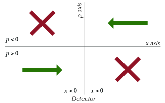
Figure 1: The classical condition for time-of-arrival measurements

Focusing on the case of a single space dimension, with the detector at $x=0$, the Kijowski metric is:

$$\rho_{d}\left(\tau\right)={\left|{\int\limits_{0}^{\infty}dp\sqrt{\frac{p}{{2\pi m}}}{e^{-\imath\frac{{{p^{2}}\tau}}{{2m}}}}{\varphi^{\left({left}\right)}}\left(p\right)}\right|^{2}}+{\left|{\int\limits_{-\infty}^{0}dp\sqrt{\frac{{-p}}{{2\pi m}}}{e^{-\imath\frac{{{p^{2}}\tau}}{{2m}}}}{\varphi^{\left({right}\right)}}\left(p\right)}\right|^{2}}$$ (4)

However while the restrictions on momentum may make sense classically, they are more troubling in quantum mechanics. It is as if we were thinking of the wave function as composed of a myriad of classical particles each of which travels like a tiny billiard ball. This would appear to be a hidden variable interpretation of quantum mechanics. This was shown to be inconsistent with quantum mechanics by Bell in 1965 [47] experimentally confirmed [48, 49, 50, 51, 52].

However, Kijowski’s metric has produced reasonable results, see for instance [53]. Therefore if we see problems with it, we need to explain the successes as well.

2.1.2 Application to Gaussian test functions

We will use Gaussian test functions (GTFs) to probe this metric. We define GTFs as normalized Gaussian functions that are solutions to the free Schrödinger equation. We will look at the results of applying Kijowski’s metric to two different cases, which we refer to as the “bullet” and “wave” variations, following Feynman’s terminology in his discussion of the double-slit experiment [54]. By “bullet” we mean a wave function which is narrowly focused around the central axis of motion; by “wave” we mean a wave function which is widely spread around the central axis of motion.

Bullets

For the bullet version we will take a GTF which starts at time $\tau=0$, centered at start position $x_{0}=-d$, with average momentum $p_{0}$, and dispersion $\sigma_{p}^{2}\ll p_{0}$. These conditions are met in the Muga, Baute, Damborenea, and Egusquiza [53] reference; they give:

$$\delta v=0.098{{cm}\mathord{\left/{\vphantom{{cm}s}}\right.\kern-1.2pt}s},{v_{0}}=10{{cm}\mathord{\left/{\vphantom{{cm}s}}\right.\kern-1.2pt}s}$$ (5)

This is typical of high-energy particles, where the free particle wave functions will have essentially no negative momentum component. The starting wave function is:

$${{\bar{\varphi}}_{0}}\left(x\right)=\sqrt[4]{{\frac{1}{{\pi\sigma_{x}^{2}}}}}{e^{\imath{p_{0}}x-\frac{1}{{2\sigma_{x}^{2}}}{{\left({x+d}\right)}^{2}}}}$$ (6)

This is taken to satisfy the free Schrödinger equation:

$$\imath\frac{\partial}{{\partial\tau}}{{\bar{\varphi}}_{\tau}}\left(x\right)=-\frac{1}{{2m}}\frac{{\partial^{2}}}{{\partial{x^{2}}}}{{\bar{\varphi}}_{\tau}}\left(x\right)$$ (7)

so is given as a function of time by:

$$\bar{\varphi}_{\tau}\left(x\right)=\sqrt[4]{\frac{1}{\pi\sigma_{x}^{2}}}\sqrt{\frac{1}{f_{\tau}^{\left(x\right)}}}e^{\imath p_{0}x-\frac{1}{2\sigma_{x}^{2}f_{\tau}^{\left(x\right)}}\left(x+d-\frac{p_{0}}{m}\tau\right)^{2}-\imath\frac{p_{0}^{2}}{2m}\tau}$$ (8)

with dispersion factor $f$ defined by:

$$f_{\tau}^{\left(x\right)}\equiv 1+\imath\frac{\tau}{m\sigma_{x}^{2}}$$ (9)

The momentum transform is:

$${{\hat{\bar{\varphi}}}_{\tau}}\left(p\right)=\sqrt[4]{{\frac{1}{{\pi\sigma_{p}^{2}}}}}{e^{\imath pd-\frac{{{\left({p-{p_{0}}}\right)}^{2}}}{{2\sigma_{p}^{2}}}-\imath\frac{{p^{2}}}{{2m}}\tau}}$$ (10)

with $\sigma_{p}\equiv\frac{1}{\sigma_{x}}$. We will use this wave function as a starting point throughout this work, referring to it as the “bullet wave function”.

In Kijowski’s notation, there is no right hand wave function since the particle started on the left. Further since the wave function is by construction narrow in momentum space we can extend the lower limit in the integral on the left from zero to negative infinity giving:

$${\rho_{d}}\left(\tau\right)={\left|{\int\limits_{-\infty}^{\infty}dp\sqrt{\frac{p}{{2\pi m}}}\sqrt[4]{{\frac{1}{{\pi\sigma_{p}^{2}}}}}{e^{\imath pd-\frac{{{\left({p-{p_{0}}}\right)}^{2}}}{{2\sigma_{p}^{2}}}-\imath\frac{{p^{2}}}{{2m}}\tau}}}\right|^{2}}$$ (11)

Since the wave function is narrowly focused, we can replace the square root in the integral by the average:

$$\sqrt{\frac{{{p_{0}}+\delta p}}{m}}\approx\sqrt{\frac{{{\text{p}}_{0}}}{m}}$$ (12)

which we can then pull outside of the integral:

$${\rho_{d}}\left(\tau\right)\approx\frac{{p_{0}}}{m}{\left|{\int\limits_{-\infty}^{\infty}{\frac{{dp}}{{\sqrt{2\pi}}}\sqrt[4]{{\frac{1}{{\pi\sigma_{p}^{2}}}}}{e^{\imath pd-\frac{{{\left({p-{p_{0}}}\right)}^{2}}}{{2\sigma_{p}^{2}}}-\imath\frac{{p^{2}}}{{2m}}\tau}}}}\right|^{2}}$$ (13)

We recognize the integral as simply the inverse Fourier transform of the momentum space form:

$${{\bar{\varphi}}_{\tau}}\left(d\right)=\sqrt[4]{{\frac{1}{{\pi\sigma_{x}^{2}}}}}\sqrt{\frac{1}{{f_{\tau}^{\left(x\right)}}}}{e^{\imath{p_{0}}d-\frac{1}{{2\sigma_{x}^{2}f_{\tau}^{\left(x\right)}}}{{\left({d-\frac{{p_{0}}}{m}\tau}\right)}^{2}}-\imath\frac{{p_{0}^{2}}}{{2m}}\tau}}$$ (14)

so:

$${\rho_{d}}\left(\tau\right)\approx\frac{{p_{0}}}{m}{\left|{{{\bar{\varphi}}_{\tau}}\left(d\right)}\right|^{2}}=\frac{{p_{0}}}{m}{{\bar{\rho}}_{\tau}}\left(d\right)$$ (15)

with the probability density being:

$${{\bar{\rho}}_{\tau}}\left(d\right)=\frac{{p_{0}}}{m}\sqrt{\frac{1}{{\pi\sigma_{x}^{2}\left({1+\frac{{\tau^{2}}}{{{m^{2}}\sigma_{x}^{4}}}}\right)}}}\exp\left({-\frac{{{\left({{\bar{x}}_{\tau}}\right)}^{2}}}{{\sigma_{x}^{2}\left({1+\frac{{\tau^{2}}}{{{m^{2}}\sigma_{x}^{4}}}}\right)}}}\right)$$ (16)

and with the average location in space:

$$\bar{x}_{\tau}\equiv-d+{v_{0}}\tau$$ (17)

We have the probability density as a function of $x$; we need it as a function of $\tau$. We therefore make the variable transformation:

$$d\tau={v_{0}}dx=\frac{{p_{0}}}{m}dx$$ (18)

And rewrite $\tau$ as the average value of $\tau$ plus an offset:

$$\tau=\bar{\tau}+\delta\tau,\bar{\tau}\equiv\frac{d}{{v_{0}}}$$ (19)

We rewrite the numerator in the density function in terms of $\delta\tau$:

$$\bar{\rho}_{\tau}\left(d\right)\approx\sqrt{\frac{1}{\pi\sigma_{x}^{2}\left|f_{\tau}^{\left(x\right)}\right|^{2}}}e^{-\frac{\left(v_{0}\delta\tau\right)^{2}}{\sigma_{x}^{2}\left|f_{\tau}^{\left(x\right)}\right|^{2}}}$$ (20)

We may estimate the uncertainty in time by expanding around the average time. Since the numerator is already only of second order in $\delta\tau$ we need only keep the zeroth order in $\delta\tau$ in the denominator:

$$\sigma_{x}^{2}\left|f_{\tau}^{\left(x\right)}\right|^{2}=\sigma_{x}^{2}+\frac{\tau^{2}}{m^{2}\sigma_{x}^{2}}\approx\frac{\tau^{2}}{m^{2}\sigma_{x}^{2}}=\frac{\left(\bar{\tau}+\delta\tau\right)^{2}}{m^{2}\sigma_{x}^{2}}\approx\frac{\bar{\tau}^{2}}{m^{2}\sigma_{x}^{2}}$$ (21)

giving:

$$\bar{\rho}_{\delta\tau}\approx\sqrt{\frac{v_{0}^{2}m^{2}\sigma_{x}^{2}}{\pi\bar{\tau}^{2}}}e^{-\frac{v_{0}^{2}m^{2}\sigma_{x}^{2}}{\bar{\tau}^{2}}\left(\delta\tau\right)^{2}}$$ (22)

We define an effective dispersion in time:

$$\bar{\sigma}_{\tau}\equiv\frac{1}{mv_{0}\sigma_{x}}\bar{\tau}$$ (23)

So we have the probability of detection as roughly:

$$\bar{\rho}_{\delta\tau}\approx\sqrt{\frac{1}{\pi\bar{\sigma}_{\tau}^{2}}}e^{-\frac{\left(\delta\tau\right)^{2}}{\bar{\sigma}_{\tau}^{2}}}$$ (24)

This is normalized to one, centered on $\tau=\bar{\tau}$, and with uncertainty:

$$\Delta\tau=\frac{1}{\sqrt{2}}\bar{\sigma}_{\tau}$$ (25)

It is interesting that the classical condition has played no essential role in this derivation. In spite of that, the result is about what we would expect from a classical particle with probability distribution $\bar{\rho}$. Therefore the implication of the experimental results in Muga and Leavens is that they are confirmation of the reasonableness of the classical approximation in general – rather than of Kijowski’s classical condition in particular.

Waves

Now consider a more wave-like Gaussian test function: slow and wide. Take $0<{p_{0}}\ll{\sigma_{p}}$ in equation 10, in fact make $p_{0}$ only very slightly greater than 0.

Our GTF is still moving to the right but very slowly. If we wait long enough – and if there were no detector in the way – it will eventually get completely past the detector. Since there is a detector, the GTF will encounter this instead. We will first assume a perfect detector with no reflection.

Use of the Kijowski distribution requires we drop the $p<0$ half of the wave function because we started on the left:

$${\varphi^{\left({wave}\right)}}\left(p\right)\Rightarrow\sqrt[4]{{\frac{1}{{\pi\sigma_{p}^{2}}}}}{e^{\imath pd-\frac{{\left({p-{p_{0}}}\right)^{2}}}{{2\sigma_{p}^{2}}}}}\theta\left(p\right)$$ (26)

We can no longer justify extending the lower bound on the left hand integral from zero to negative infinity. We have instead:

$${\rho_{d}}\left(\tau\right)={\left|{\int\limits_{0}^{\infty}dp\sqrt{\frac{p}{{2\pi m}}}\sqrt[4]{{\frac{1}{{\pi\sigma_{p}^{2}}}}}{e^{\imath pd-\frac{{{\left({p-{p_{0}}}\right)}^{2}}}{{2\sigma_{p}^{2}}}-\imath\frac{{p^{2}}}{{2m}}\tau}}}\right|^{2}}$$ (27)

This means we have dropped nearly half of the wave function and therefore expect a detection rate of only about 25%.

The integral over the momentum gives a sum over Bessel functions of fractional order; the subsequent integrals over time are distinctly non-trivial. However in the limiting case $d\to 0,p_{0}\to 0$ (the wave function starts at the detector) the distribution simplifies drastically giving:

$$\rho_{0}\left(\tau\right)={\left|{\frac{{\sqrt[4]{m}\sqrt{\sigma_{p}^{2}}\Gamma\left({\frac{3}{4}}\right)}}{{{{(2\pi)}^{3/4}}{{(m+\imath\sigma_{p}^{2}\tau)}^{3/4}}}}}\right|^{2}}$$ (28)

And this in turn is simple enough to let us compute the norm analytically:

$$\int\limits_{0}^{\infty}{d\tau\rho_{0}\left(\tau\right)}=\frac{1}{4}$$ (29)

This is exactly as expected: if we throw out half the wave function, the subsequent norms are the square of the wave function or one quarter.

This result is general. The GTF obeys the Schrödinger equation, which is norm preserving. If we throw out fraction $F$ of the wave function, the resulting wave function has norm ${\left({1-F}\right)^{2}}$. Assuming perfect detection, the Kijowski distribution will under-count the actual detections by this factor.

It is arguable that the problem is the assumption of perfect detection. However if we drill down to the actual mechanism of detection, this will involve some sort of interaction of the incoming particles with various atoms, typically involving the calculation of matrix elements of the form (e.g. Sakurai [55]):

$$\left\langle{\varphi_{\tau}^{\left({n^{\prime}l^{\prime}m^{\prime}}\right)}\left({\vec{x}}\right)}\right|\sqrt{\frac{{n_{\vec{k},\alpha}}}{{2\omega V}}}{{\vec{\varepsilon}}^{\left(\alpha\right)}}\exp\left({\imath\vec{k}\cdot\vec{x}-\imath\omega\tau}\right)\left|{\varphi_{\tau}^{\left({nlm}\right)}\left({\vec{x}}\right)}\right\rangle$$ (30)

It is difficult to make sense of the classical condition in this context. Would we have to apply it to the interaction with each atom in turn? And how would the atoms know whether they are supposed to be detecting particles coming from the left or the right? And therefore how would the unfortunate atoms know whether they should drop the upper left and bottom right quadrants on the diagram or vice versa?

2.1.3 Requirements for a time-of-arrival metric

The classical condition was introduced without justification in terms of quantum mechanics itself. As there are no cases where the rules of quantum mechanics have failed to produce correct results, this is not acceptable.

Further it is unnecessary. The probability current, discussed below (subsubsection 3.1.1), provides a conceptually sound and purely quantum mechanical approach to the problem of detection.

We therefore have to dispense entirely with the classical condition. As this is the foundation of the Kijowski class of metrics – per Muga and Leavens above – we have to dispense with the class as well.

We have however learned a bit about our requirements: we are looking for a time-of-arrival metric which satisfies the requirements:

1. Comes out of a completely quantum mechanical analysis, with no ad hoc classical requirements imposed on it.

2. Includes an account of the interaction with the detector. As Bohr pointed out during the EPR debate [56, 57], an analysis of a quantum mechanical detection must include the specifics of the apparatus. There is no well-defined value of a quantum parameter in the abstract, but only in the context of a specific measurement.

3. Conserves probability.

4. And of course, is as simple as possible given the first three requirements.

2.2 Marchewka and Schuss path integral approach

“According to our assumptions, trajectories that propagate into the absorbing boundary never return into the interval [a, b] so that the Feynman integral over these trajectories is supported outside the interval. On the other hand, the Feynman integral over the bounded trajectories in the interval is supported inside the interval. Thus the two integrals are orthogonal and give rise to no interference.” – Marchewka and Schuss [31]

We turn to an approach from Marchewka and Schuss [29, 30, 31, 32]. They use a path integral approach plus the assumption of an absorbing boundary. To compute the wave function, they use a recursive approach: computing the wave function at each step, subtracting off the absorption at each step, and so to the end.

Marchewka and Schuss start with the wave function defined over a general interval from $a\to b$. We can simplify their treatment slightly by taking $a=-\infty,b=0$. They break the time evolution up into steps of size $\epsilon$. Given the wave function at step $n$, they compute the wave function at step $n+1$ as:

$${\psi_{n+1}}\left({x_{n+1}}\right)=\int\limits_{-\infty}^{0}{d{x_{n}}{K_{\varepsilon}}\left({{x_{n+1}};{x_{n}}}\right)}{\psi_{n}}\left({x_{n}}\right)$$ (31)

The kernel can be quite general.

Marchewka and Schuss then introduce the assumption that the probability to be absorbed at each endpoint is proportional to the value of the probability to be at the end point times a characteristic length $\lambda$:

$${P_{n}}=\lambda{\left|{{\psi_{n}}\left(0\right)}\right|^{2}}$$ (32)

Using the kernel they compute the probability of absorption as:

$${P_{n}}=\frac{\varepsilon}{{2\pi{m}}}\left({\lambda\left|{\left.{{\partial_{x}}{\psi_{n}}\left(x\right)}\right|_{x=0}^{2}}\right|}\right)$$ (33)

They then shrink the wave function at the next step by an appropriate factor, the survival probability:

$${\psi_{n+1}}\left(x\right)\to\sqrt{1-{P_{n}}}{\psi_{n+1}}\left(x\right)$$ (34)

This guarantees the total probability is constant, where the total probability is the probability to be detected plus the probability to survive. This overcomes the most obvious problem with the Kijowski approach.

At the same time it represents an explicit loss of the phase information. There is nothing to keep the “characteristic length” from being complex; taking it as real is a choice. Therefore we are seeing the loss of information normally associated with the act of measurement. So we have effectively broken the total measurements at the end points down into a series of time dependent “mini-measurements” or “mini-collapses” at each time step.

Computing the product of all these infinitesimal absorptions they get the final corrected wave function as:

$$\psi_{\tau}^{\left({corrected}\right)}\left(x\right)=\exp\left({-\frac{1}{{2\pi{m}}}\int\limits_{0}^{\tau}{d\tau^{\prime}\left({{\lambda}\left|{{\left.{{\partial_{x}}{\psi_{\tau}}\left(0\right)}\right|}^{2}}\right|}\right)}}\right){\psi_{\tau}}\left(x\right)$$ (35)

They go on to apply this approach to a variety of cases, as GTFs going from left to right.

The Marchewka and Schuss approach is a significant advance over the Kijowski metric: it works at purely quantum mechanical level, it includes the detector in the analysis, and it guarantees by construction overall conservation of probability.

But at the same time the introduction of the characteristic length is a major problem for falsifiability: how do we know whether the same length should be used for SQM and for TQM?

And the trick for estimating the loss of probability at each step implicitly assumes no interference in time. This is not a problem for SQM but a point we need to keep in mind when including TQM.

We therefor further refine our requirements for a metric: we need to handle any discontinuity at the detector in a well-defined way.

2.3 Discrete approach

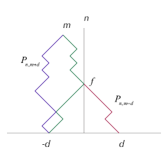
Figure 2: Reflection principle

We can handle the discontinuity at the boundary in a well-defined way by taking a discrete approach, by setting up a grid in $\tau,x$. We model quantum mechanics as a random walk on the Feynman checkerboard [58]. Feynman used steps taken at light speed; ours will travel a bit more slowly than that.

This lets us satisfy the previous requirements. And it lets us take advantage of the extensive literature on random walks (e.g. [59, 60, 61, 62]).

We will start with a random walk model for detection, take the continuous limit as the grid spacing goes to zero, Wick rotate in time, and then apply the results to a GTF. This will give us a well-defined answer for the detection rate for a GTF.

2.3.1 Random Walk

We start with a grid, index by $n\in\left[{0,1,\ldots,\infty}\right]$ in the time direction and by $m\in[-\infty,\ldots,-1,0,1,\ldots,\infty]$ in the space direction. We start with a simple coin tossing picture. We will take the probability to go left or right as equal, both $\frac{1}{2}$. $P_{nm}$ is the probability to be at position $m$ at step $n.$ It is given recursively by:

$${P_{n+1,m}}={P_{n,m-1}}/2+{P_{n,m+1}}/2$$ (36)

The number of paths from $\left(0,0\right)\to\left(n,m\right)$ is given by the binomial coefficient $\left({\begin{array}[]{c}n\\ {\frac{{n+m}}{2}}\end{array}}\right)$. We will take this as zero if $n$ and $m$ do not have the same parity, if they are not both even or both odd. If $n>\left|{m}\right|$ then $P_{nm}=0$.

The total probability to get from $\left(0,0\right)\to\left(n,m\right)$ is given by the number of paths times the probability $\frac{{1}}{2^{n}}$ for each one. In our example:

$${P_{nm}}=\left({\begin{array}[]{c}n\\ {\frac{{n+m}}{2}}\end{array}}\right)\frac{1}{{2^{n}}}$$ (37)

If we wish to start at a position other than zero, say $m^{\prime}$, we replace $m$ with $m-m^{\prime}$.

First arrival

We can model detection as the first arrival of the path at the position of the detector. We start the particle at step 0 at position $m=-d$ and position the detector at $m=0$. We take the probability of the first arrival at step $n$ when starting at position $-d$ as ${F_{n}}$.

We define the function $G_{nm}$ as the probability to arrive at position $m$ at time $n$, without having been previously detected. We can get this directly from the raw probabilities using the reflection principle (e.g. [59]) as follows:

The number of paths that start at $\left(0,-d\right)$ and get to $\left(n,m\right)$ is given by: $\left({\begin{array}[]{c}n\\ {\frac{{n+{m+d}}}{2}}\end{array}}\right)$. Now consider all paths that get to $m$ at step $n$ having first touched the detector at some step $f$. By symmetry, the number of paths from $-d\to f$ is the same as the number of paths from $d\to f$. The number of these paths is $\left({\begin{array}[]{c}n\\ {\frac{{n+\left|{m-d}\right|}}{2}}\end{array}}\right)$.

Therefore we have the number of paths that reach $m$ without first touching the line $m=0$ as ([63]):

$${G_{nm}}=\left({\left({\begin{array}[]{c}n\\ {\frac{{n+m+d}}{2}}\end{array}}\right)-\left({\begin{array}[]{c}n\\ {\frac{{n+m-d}}{2}}\end{array}}\right)}\right)\frac{1}{{2^{n}}}$$ (38)

And of course, if $\left(n,m\right)$ do not have the same parity, $G_{nm}=0$.

To get to the detector at step $n$, the particle must have been one step to the left at the previous step. It will then have a probability of $\frac{{1}}{2}$ to get the detector. So we have:

$${F_{n}}=\frac{{1}}{2}{G_{n-1,-1}}$$ (39)

giving:

$$F_{n}=\frac{d}{n}\left({\begin{array}[]{c}n\\ {\frac{{n+d}}{2}}\end{array}}\right)\frac{{1}}{2^{n}}=\frac{d}{n}{P_{nd}}$$ (40)

If the particle is already at position $0$ at step $0$ we declare that it has arrived at time zero so we have:

$$F_{0}={\delta_{d0}}$$ (41)

2.3.2 Diffusion equation

The passage to the continuum limit is well understood ([63, 62]). Define:

$$\begin{gathered}\tau=n\Delta\tau\hfill\\ x=m\Delta x\hfill\end{gathered}$$ (42)

We get the diffusion equation if we take the limit so that both $\Delta x$ and $\Delta\tau$ become infinitesimal while we keep fixed the ratio:

$${D_{0}}=\mathop{\lim}\limits_{\Delta\tau,\Delta x\to 0}\frac{{{\left({\Delta x}\right)}^{2}}}{{2\Delta\tau}}$$ (43)

This gives the diffusion equation for the probability $P$:

$$\frac{{\partial P}}{{\partial\tau}}={D_{0}}\frac{{{\partial^{2}}P}}{{\partial{x^{2}}}}$$ (44)

To further simplify we take $D_{0}=\frac{1}{2}$:

$$\frac{{\partial{P_{\tau}}}}{{\partial\tau}}=\frac{1}{2}\frac{{\partial^{2}}}{{\partial{x^{2}}}}{P_{\tau}}$$ (45)

If we start with the probability distribution ${P_{0}}\left(x-x^{\prime}\right)=\delta\left({x-x^{\prime}}\right)$ the probability distribution as a function of time is then:

$${P_{\tau}}\left({x;x^{\prime}}\right)=\frac{1}{{\sqrt{2\pi\tau}}}\exp\left({-\frac{{{\left({x-x^{\prime}}\right)}^{2}}}{{2\tau}}}\right)$$ (46)

with the probability of a first arrival at $\tau$ being given by:

$${F_{\tau}}\left({x;x^{\prime}}\right)=\frac{{\left|{x-x^{\prime}}\right|}}{{\sqrt{2\pi{\tau^{3}}}}}\exp\left({-\frac{{{\left({x-x^{\prime}}\right)}^{2}}}{{2\tau}}}\right)$$ (47)

To include the mass, scale by $\tau\to\tau^{\prime}\equiv m\tau$ giving:

$$\frac{{\partial{P_{\tau}}}}{{\partial\tau^{\prime}}}=\frac{1}{{2m}}\frac{{\partial^{2}}}{{\partial{x^{2}}}}{P_{\tau^{\prime}}}$$ (48)

and:

$${P_{\tau}}\left({x;x^{\prime}}\right)=\frac{{\sqrt{m}}}{{\sqrt{2\pi\tau}}}\exp\left({-m\frac{{{\left({x-x^{\prime}}\right)}^{2}}}{{2\tau}}}\right)$$ (49)

To get the detection rate we have to handle the scaling of the time a bit differently, since it is a probability distribution in time. The detection rate only makes sense when integrated over $\tau$, so the substitution implies:

$$\int{d\tau{F_{\tau}}\to\int{\frac{{d\tau^{\prime}}}{m}{F_{\tau^{\prime}}}}}\to\int{d\tau^{\prime}{D_{\tau^{\prime}}}}\Rightarrow{D_{\tau}}=\frac{1}{m}{F_{\tau}}$$ (50)

So we have:

$${D_{\tau}}\left({x-x^{\prime}}\right)=\frac{{\left|{x-x^{\prime}}\right|}}{\tau}\frac{{\sqrt{m}}}{{\sqrt{2\pi\tau}}}\exp\left({-m\frac{{{\left({x-x^{\prime}}\right)}^{2}}}{{2\tau}}}\right)$$ (51)

As a double check on this, we derive the detection rate directly from the diffusion equation using, again, the method of images (see appendix A).

2.3.3 Wick rotation

To go from the diffusion equation to the Schrödinger equation:

$$\imath\frac{\partial}{{\partial\tau}}\psi=-\frac{1}{{2{m}}}\frac{{\partial^{2}}}{{\partial{x^{2}}}}\psi$$ (52)

we use Wick rotation:

$$\tau\to-\imath\tau,P\to\psi$$ (53)

so we have the Wick-rotated kernel $K$:

$${K_{\tau}}\left({x;x^{\prime}}\right)=\sqrt{\frac{m}{{2\pi\imath\tau}}}\exp\left({\imath m\frac{{{\left({x-x^{\prime}}\right)}^{2}}}{{2\tau}}}\right)$$ (54)

and for the kernel for first arrival $F$:

$${F_{\tau}}\left({x;x^{\prime}}\right)=\frac{{\left|{x-x^{\prime}}\right|}}{\tau}{K_{\tau}}\left({x-x^{\prime}}\right)$$ (55)

As a second double check, we derive $F$ directly using Laplace transforms (see appendix B).

2.3.4 Application to a Gaussian test function

We start with the “bullet” GTF from our analysis of the Kijowski metric (equation 6):

$${\varphi_{0}}\left({x}\right)=\sqrt[4]{{\frac{1}{{\pi\sigma_{x}^{2}}}}}{e^{\imath{p_{0}}x-\frac{1}{{2\sigma_{x}^{2}}}{{\left({x+d}\right)}^{2}}}}$$ (56)

with:

$$\left|{d}\right|\gg{\sigma_{x}}$$ (57)

The wave function at the detector is then:

$${\varphi_{\tau}}\left(0\right)=\int\limits_{-\infty}^{0}{dx^{\prime}{F_{\tau}}\left({0;x^{\prime}}\right)}{\varphi_{0}}\left({x^{\prime}}\right)=\int\limits_{-\infty}^{0}{dx^{\prime}\frac{{\left|{0-x^{\prime}}\right|}}{\tau}{K_{\tau}}\left({0;x^{\prime}}\right)}{\varphi_{0}}\left({x^{\prime}}\right)$$ (58)

We can solve this explicitly in terms of error functions. However since $\varphi_{0}$ is strongly centered on $-d$ we can use the same trick as we did in the analysis of the Kijowski metric. We extend the upper limit of integration to $\infty$:

$${\varphi_{\tau}}\left(0\right)\approx-\frac{1}{\tau}\int\limits_{-\infty}^{\infty}{dx^{\prime}x^{\prime}{K_{\tau}}\left({0;x^{\prime}}\right)}{\varphi_{0}}\left({x^{\prime}}\right)$$ (59)

We see by inspection we can pull down the $x^{\prime}$ by taking the derivative of $\varphi_{0}$ with respect to $p_{0}$. This gives:

$${\varphi_{\tau}}\left(0\right)\approx\imath\frac{1}{{\tau}}\frac{\partial}{{\partial{p_{0}}}}\int\limits_{-\infty}^{\infty}{dx^{\prime}{K_{\tau}}\left({0;x^{\prime}}\right)}{\varphi_{0}}\left({x^{\prime}}\right)$$ (60)

We recognize the integral as the integral that propagates the free wave function from $0\to\tau$:

$${\varphi_{\tau}}\left(0\right)\approx\imath\frac{1}{{\tau}}\frac{\partial}{{\partial{p_{0}}}}\varphi_{\tau}^{\left({free}\right)}\left(0\right)$$ (61)

We have:

$$\varphi_{\tau}^{\left({free}\right)}\left(0\right)=\sqrt[4]{{\frac{1}{{\pi\sigma_{x}^{2}}}}}\sqrt{\frac{1}{{f_{\tau}^{\left(x\right)}}}}{e^{-\frac{1}{{2\sigma_{x}^{2}f_{\tau}^{\left(x\right)}}}{{\left({d-\frac{{p_{0}}}{m}\tau}\right)}^{2}}-\imath\frac{{p_{0}^{2}}}{{2m}}\tau}}$$ (62)

so the wave function for a first arrival at $\tau$ is:

$${\varphi_{\tau}}\left(0\right)\approx\left({\imath\frac{1}{{m}}\frac{{d-{v_{0}}\tau}}{{\sigma_{x}^{2}f_{\tau}^{\left(x\right)}}}+v_{0}}\right)\varphi_{\tau}^{\left({free}\right)}\left(0\right)$$ (63)

2.3.5 Metrics

We can compute the probability density to a sufficient order by expanding around the average time of arrival:

$$\bar{\tau}\equiv\frac{d}{{v_{0}}},\delta\tau\equiv\tau-\bar{\tau}$$ (64)

The first term in the expression for the $\varphi_{\tau}$ scales as $1/{\bar{\tau}}$; the second as a constant so at large $\tau$ we have:

$${\rho_{\tau}}\left(0\right)\approx v_{0}^{2}\rho_{\tau}^{\left({free}\right)}\left(0\right)$$ (65)

The result is the same as with Kijowski, except for the overall factor of $v_{0}^{2}$. Since the uncertainty is produced by normalizing this, the uncertainty in time is the same as with the bullet calculation for Kijowski. But the factor of $v_{0}^{2}$ is troubling, particularly when we recall we are using natural units so that at non-relativistic speeds this is hard to distinguish from zero.

The immediate problem is our somewhat thin-skinned approximation. The random walk can only penetrate to position $m=0$ in the grid before it is absorbed. And since the probability density is computed as the square, the result is doubly small.

Given the taking of the limit, it is perhaps more surprising that we get a finite detection rate at all. A realistic approximation would have the paths penetrating some finite distance into the detector, with the absorption going perhaps with some characteristic length – as with the Marchewka and Schuss approach.

In return for a more detailed examination of the boundary we have gotten a less physically realistic estimate. But the real problem with all three of the approaches we have looked at is their assumption of a crisp boundary between quantum and classical realms.

2.4 Implications for time-of-arrival measurements

“What is it that we human beings ultimately depend on? We depend on our words. We are suspended in language. Our task is to communicate experience and ideas to others. We must strive continually to extend the scope of our description, but in such a way that our messages do not thereby lose their objective or unambiguous character.” – Niels Bohr as cited in [64]

In reality there can be no crisp boundary between quantum and classical realms. Consider the lifespan of an atom built on classical principles, as in say Bohr’s planetary model of the atom. A classical electron in orbit around the nucleus undergoes centripetal acceleration from the nucleus; therefore emits Larmor radiation; therefore decays in towards the nucleus. The estimated lifespan is of order $10^{-11}$ seconds [65].

What keeps this from happening in the case of a quantum atom is the uncertainty principle: as the electron spirals into the nucleus its uncertainty in position is reduced so its uncertainty in momentum is increased. A larger $\Delta p$ means a larger kinetic energy. In fact the ground state energy can be estimated as the minimum total energy – kinetic plus potential – consistent with the uncertainty principle.

Since everything material is built of atoms and since there are no classical atoms there is no classical realm. And therefore it is incorrect to speak of a transition to a classical end state. No such state exists.

However classical mechanics does work very well in practice. So what we have is a problem in description. Which parts of our experimental setup – particle, source, detector, observers – can be described to acceptable accuracy using classical language; where must we use a fully quantum description?

This approach places us, with Bohr [66], firmly on the epistemological side of the measurement debate. One possible starting point is the program of decoherence [67, 68, 69, 70, 71, 72, 73, 74]. The key question for decoherence is not when does a system go from quantum to classical but rather when does a classical description become possible. Another is Quantum Trajectory Theory (QTT) [75, 76, 77, 78]. QTT, as its name suggests, is a particularly good fit with the path integral approach, the formalism we are primarily focused on here.

For the moment we will explore a more informal approach, taking advantage of the conceptual simplicity of the path integral approach. We can describe the evolution of a quantum particle in terms of the various paths it takes. In the case of the problem at hand, we visualize the paths as those that enter the detector or do not, that are reflected or are not, that leave and do not return (backflow) or return again and so on. Ultimately however each of the paths will escape permanently or else enter an entropy sink of some kind, a structure that is sufficiently macroscopic that it is no longer possible to analyze the process in terms of the individual paths. Its effects will live on, perhaps in a photo-electric cascade or a change of temperature. But the specific path will be lost like a spy in a crowd.

The entropy sink is the one essential part needed for a measurement to take place. In a quantum mechanical system information, per the no-cloning theorem, is neither created nor destroyed. But the heart of a measurement is the reduction of the complexity of the system under examination to a few numbers. Information is necessarily lost in doing this. In general it is fairly clear where this happens; typically in crossing the boundary from the microscopic to the macroscopic scale.

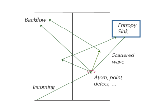
Figure 3: Global character of the measurement problem

Typical paths may cross the boundary multiple times, ultimately either being absorbed and registered (measured), lost in some way (detector inefficiency), or reflected (backflow). There will be some time delay associated with all of these cases.

This is not too far from conventional practice. A macroscopic detector functions as the entropy sink, its efficiency is usually known, and reflections are possible but minimized. In many cases the response time associated with the process of detection may not require much attention – we may only care that there was a detection. Our case is a bit trickier than that. We have to care about the time delay associated with a detection, especially if the time delay introduces some uncertainty in time in its own right.

This picture is enough to show that there can not be, in general, a local time-of-arrival operator. Suppose there is such. Consider the paths leaving it on the right, continuing to an entropic sink of some kind. If we arrange a quantum mirror of some kind (perhaps just a regular mirror), then some of the paths will return to their source. The detection rate will be correspondingly reduced. But this can only be predicted using knowledge of the global situation, of the interposed mirror. An operator local to the boundary cannot know about the mirror and therefore cannot give a correct prediction of the time-of-arrival distribution. Therefore the time-of-arrival cannot in general be given correctly by a purely local operator.

Since the fundamental laws are those of quantum mechanics, the analysis must be carried out at a quantum mechanical level – except for those parts where we can show the classical approximation suffices, usually the end states. In fact, there is no guarantee that even the end states can be adequately described in classical terms; while there are no cases – so far – of a perdurable and macroscopic quantum system, there is nothing to rule that out.

3 Effects of dispersion in time on time-of-arrival measurements

“Clearly,” the Time Traveller proceeded, “any real body must have extension in four directions: it must have Length, Breadth, Thickness, and — Duration. But through a natural infirmity of the flesh, which I will explain to you in a moment, we incline to overlook this fact. There are really four dimensions, three which we call the three planes of Space, and a fourth, Time. There is, however, a tendency to draw an unreal distinction between the former three dimensions and the latter, because it happens that our consciousness moves intermittently in one direction along the latter from the beginning to the end of our lives.” – H. G. Wells [81]

We now return to our original problem, first estimating the dispersion in time-of-arrival without dispersion in time, then with.

3.1 Time-of-arrival measurements without dispersion in time

Our efforts to correctly define a time of arrival operator have led to the conclusion that the time-of–arrival – like measurement in general – is a system level property; it is not something that can be correctly described by a local operator.

We have therefore to a certain extent painted ourselves into a corner. We would like to compute the results for the general case, but we have shown there are only specific cases. We will deal with this by trading precision for generality.

We will first assume a perfect detector, then justify the assumption.

3.1.1 Probability current in SQM

We will first compute the detection rate by using the probability current per Marchewka and Schuss [32]. We start with the Schrödinger equation:

$$\imath\frac{\partial}{{\partial\tau}}{\psi_{\tau}}\left(x\right)=-\frac{1}{{2m}}\frac{{\partial^{2}}}{{\partial{x^{2}}}}{\psi_{\tau}}\left(x\right)$$ (66)

We will assume we have in hand a wave function that includes the interaction with the detector. We define the probability of detection at clock time $\tau$ as $D_{\tau}$.

The total probability of the wave function to be found to the left of the detector at time $\tau$ is the integral of the probability density from $-\infty\to 0$. The total probability to have been detected up to time $\tau$ is the integral of $D_{\tau}$ from $0\to\tau$. Therefore by conservation of probability we have:

$$1=\int\limits_{-\infty}^{0}{dx}\psi_{\tau}^{*}\left(x\right){\psi_{\tau}}\left(x\right)+\int\limits_{0}^{\tau}{d\tau^{\prime}{D_{\tau^{\prime}}}}$$ (67)

We take the derivative with respect to $\tau$ to get:

$$D_{\tau}=-\int\limits_{-\infty}^{0}{dx\frac{{\partial\psi_{\tau}^{*}\left(x\right)}}{{\partial\tau}}{\psi_{\tau}}\left(x\right)+\psi_{\tau}^{*}\left(x\right)\frac{{\partial{\psi_{\tau}}\left(x\right)}}{{\partial\tau}}}$$ (68)

We use the Schrödinger equation:

$${D_{\tau}}=\frac{\imath}{{2m}}\int\limits_{-\infty}^{0}{dx\frac{{{\partial^{2}}\psi_{\tau}^{*}\left(x\right)}}{{\partial{x^{2}}}}{\psi_{\tau}}\left(x\right)-\psi_{\tau}^{*}\left(x\right)\frac{{{\partial^{2}}{\psi_{\tau}}\left(x\right)}}{{\partial{x^{2}}}}}$$ (69)

And integrate by parts to get the equation for the detection rate:

$${D_{\tau}}={\left.{\frac{\imath}{{2m}}\left({\frac{{\partial\psi_{\tau}^{*}\left(x\right)}}{{\partial x}}{\psi_{\tau}}\left(x\right)-\psi_{\tau}^{*}\left(x\right)\frac{{\partial{\psi_{\tau}}\left(x\right)}}{{\partial x}}}\right)}\right|_{x=0}}$$ (70)

We recognize the expression on the right as the probability current:

$${J_{\tau}}\left(x\right)=-\frac{\imath}{{2}}\left({\psi_{\tau}^{*}\left(x\right)\frac{{\partial{\psi_{\tau}}\left(x\right)}}{{\partial x}}-{\psi_{\tau}}\left(x\right)\frac{{\partial\psi_{\tau}^{*}\left(x\right)}}{{\partial x}}}\right)$$ (71)

or:

$${J_{\tau}}=\psi_{\tau}^{*}\frac{p}{{2m}}{\psi_{\tau}}-{\psi_{\tau}}\frac{p}{{2m}}\psi_{\tau}^{*}$$ (72)

so:

$$D_{\tau}=J_{\tau}$$ (73)

Note that $D_{\tau}$ can, in the general case, be negative. For instance, if the detector includes – per the previous section – a mirror of some kind there may be backflow, probability current going from right to left.

Ironically enough, this is in fact the first metric that Kijowski considered in his paper, only to reject it because it violated the classical condition 2.

3.1.2 Black box detector

Given the wave function we can compute the detection rate using the probability current. The real problem is to compute the wave function in the first place, given that this must in principle include the interaction of the particle with the detector. To treat the general case, we would like a general detector, one where the details of the interaction do not matter. We are looking for something which is a perfect black.

We can use Einstein’s clock-in-a-box, but this time run it in reverse: have the detector be a box that has a small window open for a fraction of a second then check how many particles are in the box afterward by weighing the box. The interior walls of the box provide the necessary entropy sink. We will refer to this as a black box detector .

In fact, this is a reasonable model of the elementary treatment of detection. When, for instance, we compute the rate of scattering of particles into a bit of solid angle, we assume that the particles will be absorbed with some efficiency but we do not generally worry about subtleties as time delay till a detection is registered or backflow.

3.1.3 Application to a Gaussian test function

We will take a GTF at the plane as above:

$${\varphi_{\tau}}\left(x\right)=\sqrt[4]{{\frac{1}{{\pi\sigma_{x}^{2}}}}}\sqrt{\frac{1}{{f_{\tau}^{\left(x\right)}}}}{e^{\imath{p_{0}}x-\frac{1}{{2\sigma_{x}^{2}f_{\tau}^{\left(x\right)}}}{{\left({x+d-\frac{{p_{0}}}{m}{\tau}}\right)}^{2}}-\imath\frac{{p_{0}^{2}}}{{2m}}{\tau}}}$$ (74)

An elementary application of the probability current gives the detection rate as the velocity times the probability density:

$${D_{\tau}}=\frac{{p_{0}}}{m}{\rho_{\tau}}\left(0\right)$$ (75)

This is the same as we had for the Kijowski bullet (equation 16). And it is, as noted there, also the classical rate for detection of a probability distribution impacting a wall.

Our use of the Einstein box in reverse is intended to provide a lowest common denominator for quantum measurements; it is not surprising that the lowest common denominator for quantum measurements should be the corresponding classical distribution.

We have the uncertainty in time-of-arrival as before (equation 25):

$$\Delta\tau=\frac{1}{{\sqrt{2}}}{{\bar{\sigma}}_{\tau}}=\frac{1}{{\sqrt{2}}}\frac{1}{{m{v_{0}}{\sigma_{x}}}}\bar{\tau}$$ (76)

Since we have $\bar{p}=m{v_{0}}$ and – for a minimum uncertainty wave function – ${\sigma_{p}}=\frac{1}{{\sigma_{x}}}$ we can also write:

$$\frac{{\sigma_{\tau}}}{{\bar{\tau}}}=\frac{{{\hat{\sigma}}_{p}}}{{\bar{p}}}$$ (77)

so the dispersion in momentum and in clock time are closely related, as one might expect.

While the results are the same as with the Kijowski metric (for bullet wave functions), the advantage is that we now have a clearer sense of what is actually going on and therefore what corrections we might have to make in practice. These may include (but will probably not be limited to):

1. Depletion, e.g. inefficiencies of the detector,

2. Backflow, e.g. a reflection coefficient,

3. Delay in the detection (not normally important, but significant here),

4. Self-interference of the wave function with itself,

5. Edge effects – one can imagine the incoming part of the wave function skimming along the edge of the detector for instance,

6. And of course the increasingly complex effects that result from increasingly complex models of the wave function-detector interaction.

3.2 Time-of-arrival measurements with dispersion in time

3.2.1 Quantum mechanics with uncertainty in time

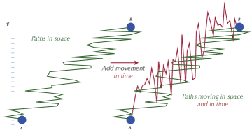
Figure 4: Paths in three and in four dimensions

Path integrals provide a natural way to extend quantum mechanics to include time in a fully covariant way. In [13] we did this by first extending the usual three-dimensional paths to four dimensions. The rest of the treatment followed from this single assumption together with the twin requirements of covariance and of consistency with known results. But as one might expect, there are a fair number of questions to be addressed along the way – making the full paper both rather long and rather technical. To make this treatment self-contained we summarize the key points here.

Feynman path integrals in four dimensions

We start with clock time, defined operationally as what the laboratory clock measures. This is the parameter $\tau$ in the Schrödinger equation, Klein-Gordon equation, path integral sums, and so on.

The normal three dimensional paths are parameterized by clock time; we generalize them to four dimensional paths, introducing the coordinate time $t$ to do so:

$${\bar{\pi}_{\tau}}\left({x,y,z}\right)\to{\pi_{\tau}}\left({t,x,y,z}\right)$$ (78)

It can be helpful to think of coordinate time as another space dimension. We will review the relationship between clock time and coordinate time at the end, once the formalism has been laid out. (This is a case where it is helpful to let the formalism precede the intuition.)

In path integrals we get the amplitude to go from one point to another by summing over all intervening paths, weighing each path by the corresponding action. The path integral with four dimensional paths is formally identical to the path integral with three dimensions, except that the paths take all possible routes in four rather than three dimensions. We define the kernel as:

$${K_{\tau}}\left({x^{\prime\prime};x^{\prime}}\right)=\mathop{\lim}\limits_{N\to\infty}\int\mathcal{D}\pi{e^{\imath\int\limits_{0}^{\tau}{d\tau^{\prime}\mathcal{L}\left[{\pi,\dot{\pi}}\right]}}}$$ (79)

We use a Lagrangian which works for both the three and four dimensional cases (see [83]):

$$\mathcal{L}\left({{x^{\mu}},{{\dot{x}}^{\mu}}}\right)=-\frac{1}{2}m{{\dot{x}}^{\mu}}{{\dot{x}}_{\mu}}-q{{\dot{x}}^{\mu}}{A_{\mu}}\left(x\right)-\frac{m}{2}$$ (80)

As usual with path integrals, to actually do the integrals we discretize clock time $\tau=\epsilon n$ and replace the integral over clock time with a sum over steps:

$$\int\limits_{0}^{\tau}{d\tau^{\prime}\mathcal{L}}\to\sum\limits_{j=0}^{n}{\mathcal{L}_{j}}$$

with:

$$\mathcal{L}_{j}\equiv-m\frac{\left(x_{j}-x_{j-1}\right)^{2}}{2\varepsilon^{2}}-q\frac{x_{j}-x_{j-1}}{\epsilon}\frac{A\left(x_{j}\right)+A\left(x_{j-1}\right)}{2}-\frac{m}{2}$$ (81)

And measure:

$$\mathcal{D}\pi\equiv\left(-\imath\frac{m^{2}}{4\pi^{2}\varepsilon^{2}}\right)^{N}\prod\limits_{n=1}^{N-1}d^{4}x_{n}$$ (82)

This gives us the ability to compute the amplitude to get from one point to another in a way that includes paths that vary in time as well as space.

Schrödinger equation in four dimensions

Usually we derive the path integral expressions from the Schrödinger equation. But here we derive the four dimensional Schrödinger equation from the short time limit of the path integral kernel, running the usual derivation in reverse and with one extra dimension. We get:

$$\imath\frac{\partial\psi_{\tau}}{\partial\tau}=-\frac{1}{{2m}}\left({\left({{p_{\mu}}-q{A_{\mu}}}\right)\left({{p^{\mu}}-q{A^{\mu}}}\right)-m^{2}}\right){\psi_{\tau}}$$ (83)

Note that here $p$ is an operator, $A$ is an external field, and $m$ is the constant operator. This equation goes back to Stueckelberg [14, 15] with further development by Feynman, Fanchi, Land, and Horwitz [16, 23, 24, 27].

We need only the free Schrödinger equation here. With the vector potential $A$ set to zero we have:

$$\imath\frac{\partial}{{\partial\tau}}{\psi_{\tau}}=-\frac{{{E^{2}}-{\overrightarrow{p}^{2}}-m^{2}}}{{2m}}{\psi_{\tau}}$$ (84)

Or spelled out:

$$\imath\frac{\partial}{{\partial\tau}}{\psi_{\tau}}\left({t,\vec{x}}\right)=\frac{1}{{2m}}\left({\frac{{\partial^{2}}}{{\partial{t^{2}}}}-{\nabla^{2}}-{m^{2}}}\right){\psi_{\tau}}\left({t,\vec{x}}\right)$$ (85)

If the left hand side were zero, the right hand side would be the Klein-Gordon equation (with $t\to\tau$). Over longer times – femtoseconds or more – the left side will in general average to zero, giving the Klein-Gordon equation as the long time limit. More formally we expect that if we average over times $\Delta\tau$ of femtoseconds or greater, we will have:

$$\int\limits_{\tau}^{\tau+\Delta\tau}{d\tau^{\prime}\int{{d^{4}}x}}\psi_{\tau}^{*}\left(x\right)\frac{{{E^{2}}-{{\vec{p}}^{2}}-{m^{2}}}}{{2m}}{\psi_{\tau}}\left(x\right)\approx 0$$ (86)

But at short times – attoseconds – we should see effects associated with uncertainty in time. This is in general how we get from a fully four dimensional approach to the usual three dimensional approach; the fluctuations in coordinate time tend to average out over femtosecond and longer time scales. But at shorter times – attoseconds – we will see the effects of uncertainty in time.

It is much the same way that in SQM quantum effects in space average out over longer time and distance scales to give classical mechanics. TQM is to SQM – with respect to time – as SQM is to classical mechanics with respect to the three space dimensions.

Wave functions in coordinate time

We need an estimate of the wave function at source, its evolution in clock time, and the rules for detection – the birth, life, and death of the wave function if you will.

Initial wave function

We start with the free Klein-Gordon equation and use the method of separation of variables to break the wave function out into a space and a time part:

$$\varphi_{0}\left(t,x\right)=\tilde{\varphi}_{0}\left(t\right)\bar{\varphi}_{0}\left(x\right)$$ (87)

Or in energy/momentum space:

$$\hat{\varphi}_{0}\left(E,p\right)=\hat{\tilde{\varphi}}_{0}\left(E\right)\hat{\bar{\varphi}}_{0}\left(p\right)$$ (88)

We assume we already have the space part by standard methods. For instance, if this is a GTF in momentum space it will look like:

$${{\hat{\bar{\varphi}}}_{\tau}}\left(p\right)=\sqrt[4]{{\frac{1}{{\pi\sigma_{p}^{2}}}}}{e^{-\imath p{x_{0}}-\frac{{{\left({p-{p_{0}}}\right)}^{2}}}{{2\sigma_{p}^{2}}}-\imath\frac{{p^{2}}}{{2m}}\tau}}$$ (89)

This plus the Klein-Gordon equation give us constraints on the time part:

$$\begin{array}[]{l}\left\langle 1\right\rangle=1\\ \bar{E}\equiv\left\langle E\right\rangle=\sqrt{m^{2}+\left\langle\vec{p}\right\rangle^{2}}\\ \left\langle E^{2}\right\rangle=\left\langle m^{2}+\vec{p}^{2}\right\rangle=m^{2}+\left\langle\vec{p}^{2}\right\rangle\end{array}$$ (90)

To get a robust estimate of the shape of the time part we assume it is the maximum entropy solution that satisfies the constraints. We used the method of Lagrange multipliers to find this getting:

$$\hat{\tilde{\varphi}}_{0}\left(E\right)=\sqrt[4]{\frac{1}{\pi\sigma_{E}^{2}}}e^{\imath\left(E-E_{0}\right)t_{0}-\frac{\left(E-E_{0}\right)^{2}}{2\sigma_{E}^{2}}}$$ (91)

with values:

$$\sigma_{E}^{2}=\sigma_{p}^{2}$$ (92)

and:

$$E_{0}=\sqrt{m^{2}+\bar{p}^{2}}$$ (93)

To get the starting wave function in time we take the inverse Fourier transform:

$$\tilde{\varphi}_{0}\left(t\right)=\sqrt[4]{\frac{1}{\pi\sigma_{t}^{2}}}e^{-\imath E_{0}\left(t-t_{0}\right)-\frac{t^{2}}{2\sigma_{t}^{2}}}$$ (94)

$$\sigma_{t}^{2}=\frac{1}{\sigma_{E}^{2}}$$ (95)

The value of the $\sigma_{t}$ will normally be of order attoseconds. We set $t_{0}=0$ as the overall phase is already supplied by the space/momentum part.

Since estimates from maximum entropy tend to be robust we expect this approach will give estimates which are order-of-magnitude correct.

Propagation of a wave function

The TQM form of the Klein-Gordon equation is formally identical to the non-relativistic Schrödinger equation with the additional coordinate time term. In momentum space one can use this insight to write the kernel out by inspection:

$${{\hat{K}}_{\tau}}\left({p^{\prime\prime};p^{\prime}}\right)={\delta^{\left(4\right)}}\left({p^{\prime\prime}-p^{\prime}}\right)\exp\left({\imath\frac{{{{p^{\prime}}^{2}}-{m^{2}}}}{{2m}}\tau}\right)\theta\left(\tau\right)$$ (96)

The coordinate space form is:

$${K_{\tau}}\left({x^{\prime\prime};x^{\prime}}\right)=-\imath\frac{{m^{2}}}{{4{\pi^{2}}{\tau^{2}}}}{e^{-\imath m\frac{{{\left({x^{\prime\prime}-x^{\prime}}\right)}^{2}}}{{2\tau}}-\imath\frac{m}{2}\tau}}\theta\left(\tau\right)$$ (97)

In both cases we have the product of a coordinate time part by the familiar space part. Spelling this out in coordinate space:

$$\begin{gathered}{K_{\tau}}\left({x^{\prime\prime};x^{\prime}}\right)={{\tilde{K}}_{\tau}}\left({{t^{\prime\prime}};{t^{\prime}}}\right){{\bar{K}}_{\tau}}\left({{{\vec{x}}^{\prime\prime}};{{\vec{x}}^{\prime}}}\right)\exp\left({-\imath\frac{m}{2}\tau}\right)\theta\left(\tau\right)\hfill\\ {{\tilde{K}}_{\tau}}\left({{t^{\prime\prime}};{t^{\prime}}}\right)=\sqrt{\frac{{\imath m}}{{2\pi\tau}}}\exp\left({-\imath m\frac{{{\left({{t^{\prime\prime}}-{t^{\prime}}}\right)}^{2}}}{{2\tau}}}\right)\hfill\\ {{\bar{K}}_{\tau}}\left({{{\vec{x}}^{\prime\prime}};{{\vec{x}}^{\prime}}}\right)={\sqrt{-\frac{\imath m}{{2\pi\tau}}}^{3}}\exp\left({\imath m\frac{{{\left({\vec{x}^{\prime\prime}-\vec{x}^{\prime}}\right)}^{2}}}{{2\tau}}}\right)\hfill\end{gathered}$$ (98)

where the space part kernel is merely the familiar non-relativistic kernel (e.g. Merzbacher [84]). The additional factor of $\exp\left({-\imath\frac{m}{2}\tau}\right)$ only contributes an overall phase which plays no role in single particle calculations.

If the initial wave function can be written as the product of a coordinate time and a three-space part, then the propagation of the three-space part is the same as in non-relativistic quantum mechanics. In general, if the free wave function starts as a direct product in time and space it stays that way.

Of particular interest here is the behavior of a GTF in time. If at clock time zero it is given by:

$$\tilde{\varphi}_{0}\left(t\right)\equiv\sqrt[4]{\frac{1}{\pi\sigma_{t}^{2}}}e^{-\imath E_{0}\left(t-t_{0}\right)-\frac{\left(t-t_{0}\right)^{2}}{2\sigma_{t}^{2}}}$$ (99)

then as a function of clock time it is:

$$\tilde{\varphi}_{\tau}\left(t\right)=\sqrt[4]{\frac{1}{\pi\sigma_{t}^{2}}}\sqrt{\frac{1}{f_{\tau}^{\left(t\right)}}}e^{-\imath E_{0}t-\frac{1}{2\sigma_{t}^{2}f_{\tau}^{\left(t\right)}}\left(t-t_{0}-\frac{E_{0}}{m}\tau\right)^{2}+\imath\frac{E_{0}^{2}}{2m}\tau}$$ (100)

with dispersion factor $f_{\tau}^{\left(t\right)}\equiv 1-\imath\frac{\tau}{m\sigma_{t}^{2}}$ and with expectation, probability density, and uncertainty:

$$\begin{array}[]{l}\left\langle{t_{\tau}}\right\rangle={t_{0}}+\frac{E}{m}\tau={t_{0}}+\gamma\tau\\ {{\tilde{\rho}}_{\tau}}\left(t\right)=\sqrt{\frac{1}{{\pi\sigma_{t}^{2}}\left({1+\frac{{\tau^{2}}}{{{m^{2}}\sigma_{t}^{4}}}}\right)}}\exp\left({-\frac{{{\left({t-\left\langle{t_{\tau}}\right\rangle}\right)}^{2}}}{{\sigma_{t}^{2}\left({1+\frac{{\tau^{2}}}{{{m^{2}}\sigma_{t}^{4}}}}\right)}}}\right)\\ {\left({\Delta t}\right)^{2}}\equiv\left\langle t^{2}\right\rangle-{\left\langle t\right\rangle^{2}}=\frac{{\sigma_{t}^{2}}}{2}\left|{1+\frac{{\tau^{2}}}{{{m^{2}}\sigma_{t}^{4}}}}\right|\end{array}$$ (101)

The behavior of the time part is given by replacing $x\to t$ and taking the complex conjugate. As noted, coordinate time behaves like a fourth space dimension, albeit one that enters with the sign of $\imath$ flipped.

Detection of a wave function

To complete the birth, life, death cycle we look at the detection of a wave function. This is obviously the place where things can get very tricky. However the general rule that coordinate time acts as a fourth space coordinate eliminates much of the ambiguity. If we were doing a measurement along the $y$ dimension and we registered a click in a detector located at $y_{detector}\pm\frac{\Delta y}{2}$ we would take this as meaning that we had measured the particle as being at position $y_{detector}$ with uncertainty $\Delta y$.

Because of our requirement of the strictest possible correspondence between coordinate time and the space dimensions, the same rule necessarily applies in coordinate time. If we have a clock in the detector with time resolution $\Delta\tau$, then a click in the detector implies a measurement of the particle at coordinate time $t=\tau$ with uncertainty $\Delta\tau.$

So the detector does an implicit conversion from coordinate time to clock time, because we have assumed we know the position of the detector in clock time. How do we justify this assumption?

The justification is that we take the clock time of the detector as being itself the average of the coordinate time of the detector:

$${\tau_{Detector}}\equiv\left\langle{t_{Detector}}\right\rangle$$ (102)

The detector will in general be made up of a large number of individual particles, each with a four-position in coordinate time and the three space dimensions. While in TQM, the individual particles may be a bit in the future or past, the average will behave as a classical variable, specifically as the clock time. This drops out of the path integral formalism, which supports an Ehrenfest’s theorem in time (again in [13]). If we take the coordinate time of a macroscopic object as the sum of the coordinate times of its component particles, the principle is macroscopically stronger. The motion in time of a macroscopic object will no more display quantum fluctuations in time than its motion in space displays quantum fluctuations in the $x,y,z$ directions.

This explains the differences in the properties of the clock time and coordinate time. The clock time is something we think of as only going forward; its corresponding energy operator is bounded below, usually by zero. But if it is really an expectation of the coordinate time of a macroscopic object, then it is not that the clock time cannot go backward, it is that it is statistically extremely unlikely to do so. The principle is the same as the argument that while the gas molecules in a room could suddenly pile up in one half of a room and leave the other half a vacuum, they are statistically extremely unlikely to do so.

Further the conjugate variable for coordinate time ${E^{\left({op}\right)}}\equiv\imath\frac{\partial}{{\partial t}}$ is not subject to Pauli’s theorem [85]. The values of $E$ – the momentum conjugate to the coordinate time $t$ – can go negative. If we look at a non-relativistic GTF:

$${{\hat{\tilde{\varphi}}}_{0}}\left(E\right)=\sqrt[4]{{\frac{1}{{\pi\sigma_{E}^{2}}}}}{e^{\imath E{t_{0}}-\frac{{{\left({E-{E_{0}}}\right)}^{2}}}{{2\sigma_{E}^{2}}}}},{\sigma_{E}}=\frac{1}{{\sigma_{t}}},{E_{0}}\approx m+\frac{{{\vec{p}}^{2}}}{{2m}}$$ (103)

the value of $m$ for an electron is about 500,000 eV, while for $\sigma_{t}$ of order attoseconds the $\sigma_{E}$ will be of order 6000 eV. Therefore the negative energy part is about $500000/6000$ or $83$ standard deviations away from the average. And therefore the likelihood of detecting a negative energy part of the wave function is zero to an excellent approximation. But not exactly zero.

So, clock time is the classical variable corresponding to the fully quantum mechanical coordinate time. They are two perspectives on the same universe.

3.2.2 Probability current in TQM

We now compute the probability current in TQM, working in parallel to the Marchewka and Schuss derivation for SQM covered above (and with similar caveats about its applicability).

By conservation of probability the sum of the detections as of clock time $\tau$ plus the total probability remaining at $\tau$ must equal one:

$$1=\int\limits_{0}^{\tau}{d\tau^{\prime}\int\limits_{-\infty}^{\infty}{dt{D_{\tau^{\prime}}}\left(t\right)}}+\int\limits_{-\infty}^{0}{dx}\int\limits_{-\infty}^{\infty}{dt}\psi_{\tau}^{*}\left({t,x}\right){\psi_{\tau}}\left({t,x}\right)$$ (104)

Again we take the derivative with respect to clock time to get:

$$\int\limits_{-\infty}^{\infty}{dt{D_{\tau}}\left(t\right)}=-\int\limits_{-\infty}^{0}{dx}\int\limits_{-\infty}^{\infty}{dt}\left({\dot{\psi}_{\tau}^{*}\left({t,x}\right){\psi_{\tau}}\left({t,x}\right)+\psi_{\tau}^{*}\left({t,x}\right){{\dot{\psi}}_{\tau}}\left({t,x}\right)}\right)$$ (105)

From the Schrödinger equation:

$$\begin{gathered}{{\dot{\psi}}_{\tau}}=-\imath\frac{1}{{2m}}\left({\frac{{\partial^{2}}}{{\partial{t^{2}}}}-\frac{{\partial^{2}}}{{\partial{x^{2}}}}}\right){\psi_{\tau}}\hfill\\ \dot{\psi}_{\tau}^{*}=\imath\frac{1}{{2m}}\left({\frac{{\partial^{2}}}{{\partial{t^{2}}}}-\frac{{\partial^{2}}}{{\partial{x^{2}}}}}\right)\psi_{\tau}^{*}\hfill\end{gathered}$$ (106)

We use integration by parts in coordinate time to show the terms in the second derivative of coordinate time cancel:

$$\imath\frac{1}{{2m}}\left({\frac{{\partial^{2}}}{{\partial{t^{2}}}}\psi_{\tau}^{*}}\right){\psi_{\tau}}-\imath\frac{1}{{2m}}\psi_{\tau}^{*}\frac{{\partial^{2}}}{{\partial{t^{2}}}}{\psi_{\tau}}\to-\imath\frac{1}{{2m}}\left({\frac{\partial}{{\partial t}}\psi_{\tau}^{*}}\right)\frac{\partial}{{\partial t}}{\psi_{\tau}}+\imath\frac{1}{{2m}}\left({\frac{\partial}{{\partial t}}\psi_{\tau}^{*}}\right)\frac{\partial}{{\partial t}}{\psi_{\tau}}=0$$ (107)

leaving:

$$\mathop{\smallint}\limits_{-\infty}^{\infty}dt{D_{\tau}}\left(t\right)=\frac{\imath}{{2m}}\mathop{\smallint}\limits_{-\infty}^{\infty}dt\mathop{\smallint}\limits_{-\infty}^{0}dx\left({\left({\frac{{{\partial^{2}}\psi_{\tau}^{*}\left({t,x}\right)}}{{\partial{x^{2}}}}}\right){\psi_{\tau}}\left({t,x}\right)-\psi_{\tau}^{*}\left({t,x}\right)\left({\frac{{{\partial^{2}}{\psi_{\tau}}\left({t,x}\right)}}{{\partial{x^{2}}}}}\right)}\right)$$ (108)

We have the probability current in the $x$ direction at each instant in coordinate time for fixed clock time:

$$j_{\tau}\left({t,x}\right)\equiv-\frac{\imath}{{2m}}\frac{{\partial\psi_{\tau}^{*}\left({t,x}\right)}}{{\partial x}}{\psi_{\tau}}\left({t,x}\right)+\frac{\imath}{{2m}}\psi_{\tau}^{*}\left({t,x}\right)\frac{{\partial{\psi_{\tau}}\left({t,x}\right)}}{{\partial x}}$$ (109)

$$j_{\tau}\left({t,x}\right)=\left({\frac{{p_{x}}}{{2m}}\psi_{\tau}^{*}\left({t,x}\right)}\right){\psi_{\tau}}\left({t,x}\right)+\psi_{\tau}^{*}\left({t,x}\right)\frac{{p_{x}}}{{2m}}{\psi_{\tau}}\left({t,x}\right)$$ (110)

What we are after is the full detection rate at a specific coordinate time:

$$D\left(t\right)=\int{d\tau{D_{\tau}}\left(t\right)}$$ (111)

If we accept that the equality in equation 108 applies at each instant in coordinate time (detailed balance) we have:

$${D_{\tau}}\left(t\right)={\left.{{j_{\tau}}\left({t,x}\right)}\right|_{x=0}}$$ (112)

giving:

$$D\left(t\right)={\left.{\int{d\tau{j_{\tau}}\left({t,x}\right)}}\right|_{x=0}}$$ (113)

Recall that the duration in clock time of a path represents the length of the path – in the discrete case the number of steps. To get the sum of all paths ending at a specific coordinate time, we need to sum over all possible path lengths. That is this integral.

As in the SQM we are assuming that once the paths enter the detector they do not return. And as with SQM, this means we have at best a reasonable first approximation. However as the SQM approximation works well in practice and as we are interested only in first corrections to SQM, this should be enough to achieve falsifiability.

3.2.3 Application to a Gaussian test function

If we construct the wave function as the direct product of time and space parts:

$${\varphi_{\tau}}\left({t,x}\right)={{\tilde{\varphi}}_{\tau}}\left(t\right){{\bar{\varphi}}_{\tau}}\left(x\right)$$ (114)

then the expression for the probability current simplifies:

$${j_{\tau}}\left({t,x}\right)=\left({\left({\frac{{p_{x}}}{{2m}}\bar{\psi}_{\tau}^{*}\left(x\right)}\right){{\bar{\psi}}_{\tau}}\left(x\right)+\bar{\psi}_{\tau}^{*}\left(x\right)\frac{{p_{x}}}{{2m}}{{\bar{\psi}}_{\tau}}\left(x\right)}\right)\tilde{\varphi}_{\tau}^{*}\left(t\right){{\tilde{\varphi}}_{\tau}}\left(t\right)$$ (115)

or:

$${D_{\tau}}\left(t\right)={{\bar{D}}_{\tau}}{{\tilde{\rho}}_{\tau}}\left(t\right)$$ (116)

Using the time wave function from equation 100 we have for the non-relativistic probability density in time:

$$\tilde{\rho}_{\tau}\left(t\right)=\sqrt{\frac{1}{\pi\sigma_{t}^{2}\left|f_{\tau}^{\left(t\right)}\right|^{2}}}e^{-\frac{1}{\sigma_{t}^{2}\left|f_{\tau}^{\left(t\right)}\right|^{2}}\left(t-\tau\right)^{2}}$$ (117)

To get the probability for detection at coordinate time $t$ we convolute clock time with coordinate time. To solve we look at the limit in long time (as with equation 21):

$$\sigma_{t}^{2}\left|f_{\tau}^{\left(t\right)}\right|^{2}=\sigma_{t}^{2}+\frac{\tau^{2}}{m^{2}\sigma_{t}^{2}}=\sigma_{t}^{2}+\frac{\left(\bar{\tau}+\delta\tau\right)^{2}}{m^{2}\sigma_{t}^{2}}\approx\frac{\left(\bar{\tau}+\delta\tau\right)^{2}}{m^{2}\sigma_{t}^{2}}\approx\frac{\bar{\tau}^{2}}{m^{2}\sigma_{t}^{2}}$$ (118)

This gives the probability density:

$${{\tilde{\rho}}_{\tau}}\left(t\right)\approx\sqrt{\frac{1}{{\pi\tilde{\sigma}_{\tau}^{2}}}}{e^{-\frac{1}{{\tilde{\sigma}_{\tau}^{2}}}{{\left({t-\tau}\right)}^{2}}}},{{\tilde{\sigma}}_{\tau}}\equiv\frac{{\bar{\tau}}}{{m{\sigma_{t}}}}$$ (119)

The convolution over $\tau$ is trivial giving:

$${{\rho_{\bar{\tau}}}\left(t\right)=\sqrt{\frac{1}{{\pi\sigma_{\tau}^{2}}}}{e^{-\frac{{{\left({t-\bar{\tau}}\right)}^{2}}}{{\sigma_{\tau}^{2}}}}}}$$ (120)

with the total dispersion in clock time being the sum of the dispersions in coordinate time and in space:

$${\sigma_{\tau}^{2}\equiv\tilde{\sigma}_{\tau}^{2}+\bar{\sigma}_{\tau}^{2}}$$ (121)

This is reasonably simple. The uncertainty is:

$$\Delta\tau=\frac{1}{{\sqrt{2}}}\sqrt{\tilde{\sigma}_{\tau}^{2}+\bar{\sigma}_{\tau}^{2}}$$ (122)

We collect the definitions for the two dispersions:

$$\begin{array}[]{c}\bar{\sigma}_{\tau}^{2}=\frac{{{\bar{\tau}}^{2}}}{{{m^{2}}{v^{2}}\sigma_{x}^{2}}}\hfill\\ \tilde{\sigma_{t}}^{2}\approx\frac{{{\bar{\tau}}^{2}}}{{{m^{2}}\sigma_{t}^{2}}}\hfill\end{array}$$ (123)

As noted, we expect the particle wave functions to have initial dispersions in energy/time comparable to their dispersions in momentum/space:

$$\sigma_{t}\sim\sigma_{x}$$ (124)

In the non-relativistic case, $v\ll 1$ the total uncertainty will be dominated by the space part. While we have looked specifically at wave functions composed of a direct product of GTFs in time and space, the underlying arguments are general. Therefore we expect that in the case of non-relativistic particles, the uncertainty in time-of-arrival will show evidence of dispersion in coordinate time, but will be dominated by the dispersion in space, because this enters with a $\frac{1}{v}$ factor and in the non-relativistic case $v$ is by definition small.

4 Applications

Single slit in time

At non-relativistic velocities, we expect that the uncertainty in time-of-arrival will be dominated by the space part. To increase the effect of uncertainty in time we can run the wave function through a single slit in time, i.e. a camera shutter which opens and closes very rapidly. In SQM, the wave function will merely be clipped and the uncertainty in time at the detector correspondingly reduced. But in TQM the reduction in $\Delta t$ will increase $\Delta E$. The increase in uncertainty in energy will cause the wave function to be more spread out in time, making the uncertainty in time at the detector arbitrarily great. The case is analogous to the corresponding single slit in space, with $\Delta E,\Delta t$ substituting for $\Delta p,\Delta x$.

In our previous paper we examined this case, but our analysis took as its starting point the Kijowski metric and associated approaches. In particular, we shifted back and forth between $q$ and $p$ in phase space in a way that we now recognize as suspect.

This obscured an important subtlety in the case of non-relativistic particles. Consider a non-relativistic particle going through a time gate. If the gate is open for only a short time, the particle must have come from an area close to the time gate. Therefore its position in space is also fairly certain. If the particle is traveling with non-relativistic velocity $v\ll 1$ then $\Delta x\sim v\Delta t\Rightarrow\Delta x\ll\Delta t$. This in turn drives up the uncertainty in momentum, $\Delta p\sim{1\mathord{\left/{\vphantom{1{\Delta x}}}\right.\kern-1.2pt}{\Delta x}}$, leading to increased uncertainty in time at the detector, even for SQM.

To avoid this problem, we replace the gate with a time-dependent source. We let the particles propagate for a short time past the source, then compare the expected uncertainties without and with dispersion in time. The basic conclusion of the previous work is unchanged: we can make the difference between the two cases arbitrarily large. We work out the details in appendix C.

Double slit in time

The double slit experiment is often cited as the key experiment for quantum mechanics (mostly famously by Feynman [54]). And Lindner’s “Attosecond Double-Slit Experiment” [86] provided a key inspiration for the current work, in that it showed we could now explore interference effects at the necessary attosecond scale. Building on this, Palacios et al [87] have proposed an experiment using spin-correlated pairs of electrons which takes advantage of the electrons being indistinguishable to look for interference in the time-energy domain.

Both experiments use the standard quantum theory to do the analysis of interference in the time/energy dimension. Horwitz [25, 88, 27] notes that as time is a parameter in standard quantum mechanics it is difficult to fully justify this analysis. He provides an alternative analysis in terms of the Stueckelberg equation (our eq 83) which is not subject to this objection. He gets the same spacing for the fringes as Lindner found.

Unfortunately for this investigation since the fringe spacing is the same using the Lindner’s analysis or the one here the fringe pattern does not let us distinguish between the two approaches; it contributes nothing to falsifiability.

We do expect, from the analysis of the single slit experiment, that the individual fringes will be smoothed out from the additional dispersion in time: the brights less bright, the darks less dark. However the contribution of this effect to falsifiability is already covered by the analysis of the single slit experiment.

Quantum electrodynamics

While the above is sufficient to establish that we can detect the effects of uncertainty in time, it is clear that the strongest and most interesting effects will be seen at high energies and relativistic speeds, where the effects of quantum field theory (QFT) will need to be taken into account.

In the previous paper, we looked at the QFT approach to systems of spinless, massive particles. We were able to extend TQM to QFT in a straightforward and unambiguous way. We also showed that we recover the usual Feynman rules in the appropriate limit. And that we will see various interesting effects from the additional uncertainty in time.

One obvious concern was that the additional dimension in the loop integrals might make the theory still more divergent than QFT already is, perhaps even unrenormalizable. But in the spin 0 massive case we do not see the usual ultraviolet (UV) divergences: the combination of uncertainty in time, entanglement in time, and the use of finite initial wave functions (rather than plane waves or $\delta$ functions) suppresses the UV divergences without the need for regularization.

The extension to spin 1/2 particles and to photons appears to be straightforward. We expect to see the various effects of time-as-observable for spin 1/2 particles and photons: interference in time, entanglement in time, correlations in time, and so on. We will also look at the implications for spin correlations, symmetry/anti-symmetry under exchange of identical particles, and the like.

One caveat: if we analyze the photon propagator using the familiar trick of letting the photon mass $\mu\to 0$[89] we can see from inspection of the $\frac{1}{2\mu}$ factor in the propagator in momentum space:

$${K_{\tau}}\left({k;k^{\prime}}\right)=\exp\left({\imath\frac{{{k^{2}}-{\mu^{2}}}}{{2\mu}}\tau}\right){\delta^{4}}\left({k-k^{\prime}}\right)$$ (125)

that excursions off-shell will be severely penalized. This in turn will limit the size of the effects of TQM in experiments such as the single slit in time. Such experiments are therefore better run with massive particles, the more massive the better in fact.

In this paper we have estimated the initial wave functions in time using dimensional and maximum entropy arguments. Once TQM has been extended to include QED, we should be able to combine the standard QED results with these to serve as the zeroth term in a perturbation expansion, then compute first and higher corrections using the standard methods of time-dependent perturbation theory.

This should open up a wide variety of interesting experiments.

General Relativity

As noted in the introduction, TQM is a part of the relativistic dynamics program so can draw on the extensive relativistic dynamics literature. In particular we can take advantage of Horwitz’s extension of relativistic dynamics to General Relativity for single particles, the classical many body problem, and the quantum many body problem [90, 91, 92].

There would appear to be an interesting complementarity between the work of Horwitz and this work. First, TQM supplies an explicit source for the invariant monotonic parameter $\tau$ so that we do not need to introduce this as an additional assumption. Second, TQM avoids the UV divergences which have created significant difficulties for work to extend QFT to General Relativity. Therefore an appropriate combination of the two approaches might provide useful insights into the extension of QFT to General Relativity.

5 Discussion

“It is not surprising that our language should be incapable of describing the processes occurring within the atoms, for, as has been remarked, it was invented to describe the experience of daily life, and these consist only of processes involving exceedingly large numbers of atoms. Furthermore, it is very difficult to modify our language so that it will be able to describe these atomic processes, for words can only describe things of which we can form mental pictures, and this ability, too, is a result of daily experience. Fortunately, mathematics is not subject to this limitation, and it has been possible to invent a mathematical scheme — the quantum theory — which seems entirely adequate for the treatment of atomic processes…” – Werner Heisenberg [93]

Falsifiability

The Heisenberg uncertainty principle (HUP) in time follows directly from quantum mechanics and relativity. This was clear to both Einstein and Bohr in 1930. However quantum mechanics since then has not in general included it. Given that the relevant attosecond time scales have been too small to work with – until recently – this is reasonable enough.

However it is now possible to look at the time at the relevant scales; it is therefore necessary to do so, if we are understand either time or quantum mechanics. The specific predictions made here are based on only covariance and the requirement of consistency with existing results, they are by construction without free parameters. They should therefore provide at a minimum a reasonable order-of-magnitude target.

The time-of-arrival experiment we have focused on here provides merely the most obvious line of attack. Essentially any experiment looking at time-dependent phenomena is a potential candidate. For instance in Auletta [94] there are about three hundred foundational experiments; most can be converted into a test of uncertainty in time by replacing an $x$ with a $t.$ Examples include the single slit in time, the double slit in time, and so on. One may also look at variations intended to multiply normally small effects, as experiments using resonance or diffraction effects.

Implications of negative result striking

From symmetry, one may argue that a positive result is the more likely, but even a negative result would be interesting.

For instance, assume we have established there is no HUP in time in one frame. Consider the same experiment from another frame moving at high velocity relative to the first. Consider say a Gaussian test function (GTF) in $x$ in the first; make a Lorentz boost of this into the second frame. The Lorentz boost will transform $x\to\gamma\left(x-v\tau\right)$. This will turn the uncertainty in space into a mixture of uncertainty in space and in time. We then look for uncertainty in time in the boosted frame.

If the HUP in time is also rejected in the second, how do we maintain the principle of covariance? If the HUP in time is present in the second frame, then we can defined a preferred frame as the one in which HUP in time is maximally falsified. Such a preferred frame is anathema to general relativity.

Therefore exploring the precise character of the negative result – uniform across frames, more in some frames than others, and so on – would itself represent an interesting research program.

Positive result would have significant practical applications

If on the other hand, the wave function extends in time, this would not only be interesting from the point of view of fundamental physics, it would open up a variety of practical applications. For instance, there would be an additional channel for quantum communication systems to use. Memristors and other time-dependent circuit elements would show interesting effects. In attosecond chemistry and biochemistry we would expect to see forces of anticipation and regret; if the wave function extends in time, it will cause interactions to start earlier and end later than would otherwise be the case. The mysteries of protein folding could be attacked from a fresh perspective and perhaps unexpected temporal subtleties found.

The applications in quantum computing are particularly interesting. Quantum computers will need to compensate for the effects of decoherence along the time dimension. But they should also be able to take advantage of additional computing opportunities along the time dimension. And if we have a deeper understanding of the relationship between time and measurement, we may find opportunities to “cut across the diagonal” in the design of quantum computers.

I thank my long time friend Jonathan Smith for invaluable encouragement, guidance, and practical assistance.

I thank Ferne Cohen Welch for extraordinary moral and practical support.

I thank Martin Land, L. P. Horwitz, and the other organizers and participants of the International Association for Relativistic Dynamics (IARD) 2020 Conference for encouragement, useful discussions, and hosting a talk on this paper at the IARD 2020 conference.

I thank the reviewer who drew my attention to Horwitz’s [90].

I thank Steven Libby for several useful conversations.

I thank Larry Sorensen for many helpful references. I thank Ashley Fidler for helpful references to the attosecond physics literature.

And I thank Avi Marchewka for an interesting and instructive conversation about various approaches to time-of-arrival measurements.

And I note none of the above are in any way responsible for any errors of commission or omission in this work.

.

Appendix A Direct computation of the detection rate in diffusion

We use conservation of probability and the method of images to make a direct computation of the detection rate in the case of diffusion. The approach is similar to the one used by Marchewka and Schuss to compute the probability current (subsection 3.1.1), although the context is classical rather than quantum.

Define ${G_{\tau}}\left(x\right)$ as the probability to get from $d\to x$ without touching the detector at $0$. We get $G$ from the method of images by the same logic as in the discrete case:

$${G_{\tau}}\left(x\right)={P_{\tau}}\left({x;-d}\right)-{P_{\tau}}\left({x;d}\right)$$ (126)

$G$ obeys the diffusion equation:

$$\frac{{\partial{G_{\tau}}}}{{\partial\tau}}=\frac{1}{{2m}}\frac{{\partial^{2}}}{{\partial{x^{2}}}}{G_{\tau}}$$ (127)

Take $D_{\tau}$ as the rate of detection at $\tau$. From conservation of probability we have:

$$1=\int\limits_{-\infty}^{0}{dx{G_{\tau}}\left(x\right)}+\int\limits_{0}^{\tau}{d\tau^{\prime}{D_{\tau^{\prime}}}}$$ (128)

Take the derivative with respect to $\tau$ and apply the diffusion equation:

$${D_{\tau}}=-\int\limits_{-\infty}^{0}{dx\frac{{\partial{G_{\tau}}}}{{\partial\tau}}\left(x\right)}=-\int\limits_{-\infty}^{0}{dx\frac{1}{{2m}}\frac{{\partial^{2}}}{{\partial{x^{2}}}}G}$$ (129)

Since the term on the right is the integral of a derivative we have:

$${D_{\tau}}=-\frac{1}{{2m}}{\left.{\frac{\partial}{{\partial x}}G}\right|_{x=0}}$$ (130)

By using the explicit form for $P$ (equation 49) we get:

$${D_{\tau}}=\frac{d}{\tau}{P_{\tau}}\left(d\right)$$ (131)

as above (equation 51).

Appendix B Alternate derivation of the detection amplitude

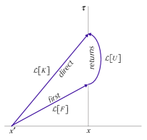
Figure 5: Computation of amplitude for first arrival by using the Laplace transform

We compute $F$ by using the Laplace transform.

To get to any specific point $x$ we have to get to the point the first time, then return to it zero or more times. Therefore we can write the full kernel $K$ as the convolution of the kernel $F$ to arrive for the first time and the kernel $U$ to return zero or more times:

$${K_{\tau}}\left({x;x^{\prime}}\right)=\int\limits_{0}^{\tau}{d\tau^{\prime}{U_{\tau^{\prime}}}\left(x\right){F_{\tau^{\prime}}}\left({x;x^{\prime}}\right)}$$ (132)

Since the kernel is invariant under space translation:

$$\begin{gathered}{K_{\tau}}\left({x;x^{\prime}}\right)={K_{\tau}}\left({x-x^{\prime}}\right)\hfill\\ {F_{\tau^{\prime}}}\left({x;x^{\prime}}\right)={F_{\tau}}\left({x-x^{\prime}}\right)\hfill\end{gathered}$$ (133)

and:

$${U_{\tau}}\left(x\right)={U_{\tau}}\left(0\right)={K_{\tau}}\left(0\right)$$ (134)

we can simplify the convolution to:

$${K_{\tau}}\left({x-x^{\prime}}\right)=\int\limits_{0}^{\tau}{d\tau^{\prime}{U_{\tau^{\prime}}}F_{\tau^{\prime}}\left({x-x^{\prime}}\right)}$$ (135)

The Laplace transform of $K$ is the product of the Laplace transform of $U$ and $F$:

$$\mathcal{L}\left[K\right]=\mathcal{L}\left[U\right]\mathcal{L}\left[F\right]$$ (136)

The free kernel is:

$${K_{\tau}}\left(x\right)=\sqrt{\frac{m}{{2\pi\imath\tau}}}\exp\left({\imath m\frac{{x^{2}}}{{2\tau}}}\right)$$ (137)

with Laplace transform:

$$\mathcal{L}\left[K\right]=-\left({-{1^{3/4}}}\right)\frac{{e^{\left({-1+\imath}\right)\sqrt{ms}\left|x\right|}}}{{\sqrt{2}\sqrt{s}}}\sqrt{m}$$ (138)

To get the Laplace transform of $U$ take the $x=0$ case:

$$\mathcal{L}\left[U\right]=-\frac{{\left({-{1^{3/4}}}\right)}}{{\sqrt{2}\sqrt{s}}}\sqrt{m}$$ (139)

Therefore we have the Laplace transform for $F$:

$$\mathcal{L}\left[F\right]={e^{\left({-1+\imath}\right)\sqrt{ms}\left|x\right|}}$$ (140)

and we get $F_{\tau}$ from the inverse Laplace transform:

$$\begin{gathered}\hfill\\ {F_{\tau}}=\frac{\left|x\right|}{\tau}{K_{\tau}}\left(x\right)\hfill\end{gathered}$$ (141)

Appendix C Single slit in time

We compare the results of the single slit in time in SQM and TQM. We model the single slit in time as a particle source located at $x=-d$, emitting particles with momentum $p_{0}$ in the $x$-direction, velocity ${v_{0}}=\frac{{p_{0}}}{m}$.

In the SQM case, we assume that the wave function is emitted with probability $\bar{G}_{\tau}$:

$$\bar{G}\left(\tau\right)\equiv\frac{1}{{\sqrt{2\pi{W^{2}}}}}\exp\left({-\frac{{\tau^{2}}}{{2{W^{2}}}}}\right)$$ (142)

This is normalized to one, with uncertainty in time $\Delta\tau=W$.

To extend to TQM we will replace this probability with an amplitude:

$${{\tilde{\varphi}}_{0}}\left(t_{0}\right)=\sqrt[4]{{\frac{1}{{\pi\sigma_{t}^{2}}}}}\exp\left({-\imath E_{0}t_{0}-\frac{{t_{0}^{2}}}{{2\sigma_{t}^{2}}}}\right)$$ (143)

This has probability distribution and uncertainty:

$$\begin{gathered}{{\tilde{\rho}}_{0}}\left({t_{0}}\right)=\sqrt{\frac{1}{{\pi\sigma_{t}^{2}}}}\exp\left({-\frac{{t_{0}^{2}}}{{\sigma_{t}^{2}}}}\right)\\ \Delta t=\frac{{\sigma_{t}}}{{\sqrt{2}}}\end{gathered}$$ (144)

We will take ${\sigma_{t}}=\sqrt{2}W$ so that the uncertainty from the gate is equal to the uncertainty from the initial distribution in coordinate time, to make the comparison as fair as possible.

The detector will be positioned at $x=0$. The average time of arrival is $\bar{t}=\bar{\tau}=\frac{d}{{v_{0}}}$. We are interested in the uncertainty in time at the detector as defined above for SQM and TQM.

C.1 Single slit in time in SQM

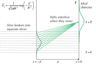
Figure 6: Single slit in time in SQM

In SQM the wave function extends in only the three space dimensions. If we break time up into slices, there is no interference across slices. At each time slice, there is an amplitude for paths from that slice to get to the detector. But if we look at the individual paths emitted during that time slice, some get to the detector at one time, some at an earlier or a later time. At the detector all paths that arrive at the same clock time interfere, constructively or destructively, as may happen. This is the picture used by Lindner et al in their analysis. The peaks in the incoming electric wavelet ejected electrons at different times, but when the electrons ejected from different times arrived at the detector at the same time they interfered.

To make this specific, we will use a simple model.

For convenience, we will assume that the source has an overall time dependency of $\exp\left({-\imath\frac{{p_{0}^{2}}}{{2m}}{\tau_{G}}}\right)$ so that our initial wave function is:

$${{\bar{\varphi}}_{G}}\left({x_{G}}\right)=\sqrt[4]{{\frac{1}{{\pi\sigma_{x}^{2}}}}}{e^{\imath{p_{0}}{x_{G}}-\frac{1}{{2\sigma_{x}^{2}}}x_{G}^{2}-\frac{{p_{0}^{2}}}{{2m}}{\tau_{G}}}}$$ (145)

This is normalized to one at the start:

$$1=\int{d{x_{G}}\varphi_{G}^{*}\left({x_{G}}\right){\varphi_{G}}\left({x_{G}}\right)}$$ (146)

So the particle will have a total probability of being emitted of one:

$$1=\int\limits_{-\infty}^{\infty}{d\tau{{\bar{G}}_{\tau}}\int{d{x_{G}}\varphi_{G}^{*}\left({x_{G}}\right){\varphi_{G}}\left({x_{G}}\right)}}$$ (147)

The amplitude at the detector from a single moment at the gate will be given by:

$${{\bar{\varphi}}_{DG}}\left(x\right)=\sqrt[4]{{\frac{1}{{\pi\sigma_{x}^{2}}}}}\sqrt{\frac{1}{{f_{DG}^{\left(x\right)}}}}{e^{\imath{p_{0}}x-\frac{1}{{2\sigma_{x}^{2}f_{DG}^{\left(x\right)}}}{{\left({x+d-{v_{0}}{\tau_{DG}}}\right)}^{2}}-\imath\frac{{p_{0}^{2}}}{{2m}}{\tau_{D}}}}$$ (148)

with ancillary definitions:

$$\begin{gathered}{\tau_{DG}}\equiv{\tau_{D}}-{\tau_{G}}\hfill\\ f_{DG}^{\left(x\right)}=1+\imath\frac{{\tau_{DG}}}{{m\sigma_{x}^{2}}}\hfill\end{gathered}$$ (149)

We have:

$$x+d-{v_{0}}\left({{\tau_{D}}-{\tau_{G}}}\right)=-{v_{0}}\left({\delta\tau-{\tau_{G}}}\right)$$ (150)

Both $\delta\tau$ and $\tau_{G}$ are expected small. We can therefore justify taking:

$$f_{DG}^{\left(x\right)}=1+\imath\frac{{\tau_{DG}}}{{m\sigma_{x}^{2}}}\approx f_{\bar{\tau}}^{\left(x\right)}=1+\imath\frac{{\bar{\tau}}}{{m\sigma_{x}^{2}}}$$ (151)

Giving:

$${{\bar{\varphi}}_{DG}}\left(x\right)=\sqrt[4]{{\frac{1}{{\pi\sigma_{x}^{2}}}}}\sqrt{\frac{1}{{f_{\vec{\tau}}^{\left(x\right)}}}}{e^{\imath{p_{0}}x-\frac{{v_{0}^{2}}}{{2\sigma_{x}^{2}f_{\vec{\tau}}^{\left(x\right)}}}{{\left({\delta\tau-{\tau_{G}}}\right)}^{2}}-\imath\frac{{p_{0}^{2}}}{{2m}}{\tau_{D}}}}$$ (152)

To get the full wave function at the detector we need to take the convolution of this with the gate function:

$${{\bar{\psi}}_{D}}\left(x\right)=\int\limits_{-\infty}^{\infty}{d{\tau_{G}}\bar{G}\left({\tau_{G}}\right){{\bar{\varphi}}_{DG}}\left(x\right)}$$ (153)

giving:

$${{\bar{\psi}}_{D}}\left(x\right)=\frac{{\sigma_{x}}}{{v_{0}}}\sqrt[4]{{\frac{1}{{\pi\sigma_{x}^{2}}}}}\frac{1}{{\sqrt{2\pi\left({\frac{{\sigma_{x}^{2}}}{{v_{0}^{2}}}+{W^{2}}+\imath\frac{{\bar{\tau}}}{{mv_{0}^{2}}}}\right)}}}\exp\left({\imath{p_{0}}x-\frac{{{\left({\delta\tau}\right)}^{2}}}{{2\left({\frac{{\sigma_{x}^{2}}}{{v_{0}^{2}}}+{W^{2}}+\imath\frac{{\bar{\tau}}}{{mv_{0}^{2}}}}\right)}}-\imath\frac{{p_{0}^{2}}}{{2m}}{\tau_{D}}}\right)$$ (154)

We can see that the effect of the gate is to increase the effective dispersion in space:

$$\frac{{\sigma_{x}^{2}}}{{v_{0}^{2}}}\to\frac{{\sigma_{x}^{2}}}{{v_{0}^{2}}}+{W^{2}}\Rightarrow\sigma_{x}^{2}\to\Sigma_{x}^{2}\equiv\sigma_{x}^{2}+v_{0}^{2}{W^{2}}$$ (155)

The gate effectively adds an uncertainty of $vW$ to the original uncertainty in space. As $vW$ is about the distance a particle would cross while the gate is open, this is reasonable.

We get then as the associated uncertainty in time (eq: 76):

$$\Delta\tau=\frac{1}{{\sqrt{2}}}{{\bar{\Sigma}}_{\tau}}=\frac{1}{{\sqrt{2}}}\frac{1}{{m{v_{0}}{\Sigma_{x}}}}\bar{\tau}$$

The longer the gate stays open the greater the resulting uncertainty in time at the detector. The shorter the gate stays open the less the uncertainty in time at the detector, with the minimum being the uncertainty for a free GTF released at the time and location of the gate.

C.2 Single slit in time in TQM

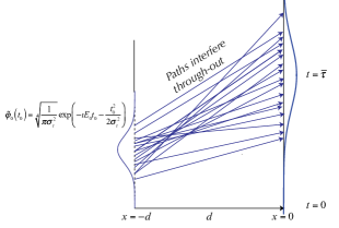
Figure 7: Single slit in time in TQM

In TQM the wave function extends in all four dimensions. There is interference across time so it is no longer legitimate to break time up into separate slices (except for purposes of analysis of course). We will take the source as centered at a specific moment in coordinate time, $t=0$.

We can write the four dimensional wave function as the product of the time (eq: 143) and space parts:

$${\varphi_{0}}\left({{t_{0}},{{\vec{x}}_{0}}}\right)={\tilde{\varphi}_{0}}\left({t_{0}}\right){\bar{\varphi}_{0}}\left({{\vec{x}}_{0}}\right)$$ (156)

The space part is as above for clock time $\tau=0$.

The time part at clock time $\tau$ is:

$${{\tilde{\varphi}}_{\tau}}\left(t\right)=\sqrt[4]{{\frac{1}{{\pi\sigma_{t}^{2}}}}}\sqrt{\frac{1}{{f_{\tau}^{\left(t\right)}}}}{e^{-\imath{E_{0}}t-\frac{1}{{2\sigma_{t}^{2}f_{\tau}^{\left(t\right)}}}{{\left({t-\frac{{E_{0}}}{m}\tau}\right)}^{2}}}}$$ (157)

For a non-relativistic particle $\frac{E}{m}\approx 1$. The treatment in subsection 3.2.3 applies giving the uncertainty in time at the detector as:

$$\Delta\tau=\frac{1}{{\sqrt{2}}}\sqrt{\tilde{\sigma}_{\tau}^{2}+\bar{\sigma}_{\tau}^{2}}$$ (158)

with contributions from the space and time parts of:

$$\begin{gathered}\bar{\sigma}_{\tau}^{2}=\frac{{{\bar{\tau}}^{2}}}{{{m^{2}}{v^{2}}\sigma_{x}^{2}}}\hfill\\ \tilde{\sigma}_{\tau}^{2}=\frac{{{\bar{\tau}}^{2}}}{{{m^{2}}\sigma_{t}^{2}}}=\frac{{{\bar{\tau}}^{2}}}{{2{m^{2}}{W^{2}}}}\hfill\end{gathered}$$ (159)

So we have the scaled uncertainty in time as:

$$\frac{{\Delta\tau}}{{\bar{\tau}}}=\frac{1}{{\sqrt{2}}}\frac{1}{m}\sqrt{\frac{1}{{{v^{2}}\sigma_{x}^{2}}}+\frac{1}{{2{W^{2}}}}}$$ (160)

We can see that when $W\sim v\sigma_{x}$ the effects of dispersion in time will be comparable to those from dispersion in space. And as $W\to 0$, the uncertainty in time at the detector will be dominated by the width of the gate in time, going as $\frac{1}{W}$.

So the intrinsic uncertainty in space of a GTF creates a corresponding minimum uncertainty in time at the detector given by $\bar{\sigma}_{\tau}$. In SQM the effects of the gate drop to zero as $W\to 0$ while in TQM they go to infinity. In SQM the wave function is clipped in time; in TQM it is diffracted.

We therefore have the unambiguous signal – even in the non-relativistic case – that we need to achieve practical falsifiability.

References

- [1] Feynman R P 1965 The Character of Physical Law (Modern Library) ISBN 0 679 60127 9
- [2] Schilpp P A and Bohr N 1949 Discussion with Einstein on Epistemological Problems in Atomic Physics (Evanston: The Library of Living Philosophers) pp 200–241
- [3] Pais A 1982 Subtle is the Lord: The Science and Life of Albert Einstein (Oxford University Press)
- [4] Hilgevoord J 1996 American Journal of Physics 64 1451–1456
- [5] Hilgevoord J 1998 American Journal of Physics 66 396–402
- [6] Busch P 2001 The Time Energy Uncertainty Relation (Berlin: Springer-Verlag) pp 69–98 Lecture Notes in Physics
- [7] Pauli W 1980 General Principles of Quantum Mechanics (Springer-Verlag) URL http://www.springer.com/us/book/9783540098423
- [8] Dirac P A M 1958 General Principles of Quantum Mechanics 4th ed International series of monographs on physics (Oxford, Clarendon Press)
- [9] Muga J G, Sala Mayato R and Egusquiza I L 2002 Time in Quantum Mechanics (Berlin; New York: Springer) ISBN 3540432949
- [10] Muga J G, Sala Mayato R and Egusquiza I L 2008 Time in Quantum Mechanics - Vol 2 (Berlin; New York: Springer-Verlag) ISBN 3540734724 9783540734727 0075-8450 ;
- [11] Ossiander M, Siegrist F, Shirvanyan V, Pazourek R, Sommer A, Latka T, Guggenmos A, Nagele S, Feist J, Burgdörfer J, Kienberger R and Schultze M 2016 Nature Physics 13 280
- [12] Abbott E A 1884 Flatland: A Romance of Many Dimensions (Seeley and Co. of London)
- [13] Ashmead J 2019 Journal of Physics: Conference Series 1239 012015 URL https://iopscience.iop.org/article/10.1088/1742-6596/1239/1/012015
- [14] Stueckelberg E C G 1941 Helv. Phys. Acta. 14 51
- [15] Stueckelberg E C G 1941 Helv. Phys. Acta. 14 322–323
- [16] Feynman R P 1948 Rev. Mod. Phys. 20(2) 367–387
- [17] Feynman R P 1949 Phys Rev 76 749–759
- [18] Feynman R P 1949 Phys Rev 76 769–789
- [19] Feynman R P 1950 Physical Review 80 440–457
- [20] Horwitz L P and Piron C 1973 Helvetica Physica Acta 46
- [21] Fanchi J R and Collins R E 1978 Found Phys 8 851–877
- [22] Fanchi J R 1993 Found. Phys. 23
- [23] Fanchi J R 1993 Parameterized Relativistic Quantum Theory (Fundamental Theories of Physics vol 56) (Kluwer Academic Publishers)
- [24] Land M C and Horwitz L P 1996 ArXiv e-prints (Preprint hep-th/9601021v1) URL http://lanl.arxiv.org/abs/hep-th/9601021v1
- [25] Horwitz L P 2006 Physics Letters A 355 1–6 (Preprint quant-ph/0507044) URL http://arxiv.org/abs/quant-ph/0507044
- [26] Fanchi J R 2011 Found Phys 41 4–32
- [27] Horwitz L P 2015 Relativistic Quantum Mechanics Fundamental Theories of Physics (Springer Dordrecht Heidelberg New York London)
- [28] Kijowski J 1974 Reports on Mathematical Physics 6 361–386
- [29] Marchewka A and Schuss Z 1998 Phys.Lett. A240 177–184 (Preprint quant-ph/9708034) URL https://arxiv.org/abs/quant-ph/9708034
- [30] Marchewka A and Schuss Z 1999 Phys. Lett. A 65 042112 (Preprint quant-ph/9906078) URL https://arxiv.org/abs/quant-ph/9906078
- [31] Marchewka A and Schuss Z 1999 ArXiv e-prints (Preprint quant-ph/9906003) URL https://arxiv.org/abs/quant-ph/9906003
- [32] Marchewka A and Schuss Z 2000 Phys. Rev. A 61 052107 (Preprint quant-ph/9903076) URL https://arxiv.org/abs/quant-ph/9903076
- [33] Muga J G and Leavens C R 2000 Physics Reports 338 353–438
- [34] Baute A D, Mayato R S, Palao J P, Muga J G and Egusquiza I L 2000 Phys.Rev.A 61 022118 (Preprint quant-ph/9904055) URL https://arxiv.org/abs/quant-ph/9904055
- [35] Baute A D, Egusquiza I L, Muga J G and Sala-Mayato R 2000 Phys. Rev. A 61 052111 (Preprint quant-ph/9911088) URL https://arxiv.org/abs/quant-ph/9911088
- [36] Baute A D, Egusquiza I L and Muga J G 2001 Phys. Rev. A 64 012501 (Preprint quant-ph/0102005) URL https://arxiv.org/abs/quant-ph/0102005
- [37] Ruggenthaler M, Gruebl G and Kreidl S 2005 Journal of Physics A: Mathematical and General 38 (Preprint quant-ph/0504185) URL https://arxiv.org/abs/quant-ph/0504185
- [38] Anastopoulos C and Savvidou N 2006 J. Math. Phys. 47 122106 (Preprint quant-ph/0509020) URL https://arxiv.org/abs/quant-ph/0509020
- [39] Yearsley J M 2010 ArXiv e-prints (Preprint 1012.2575v1) URL https://arxiv.org/abs/1012.2575v1
- [40] Kiukas J, Ruschhaupt A, Schmidt P O and Werner R F 2012 Journal of Physics A: Mathematical and Theoretical 45 (Preprint 1109.5087) URL https://arxiv.org/abs/1109.5087
- [41] Yearsley J M, Downs D A, Halliwell J J and Hashagen A K 2011 Phys. Rev. A 84 022109 (Preprint 1106.4767) URL https://arxiv.org/abs/1106.4767
- [42] Halliwell J J, Evaeus J, London J and Malik Y 2015 Physics Letters A 379 2445 (Preprint 1504.02509) URL https://arxiv.org/abs/1504.02509
- [43] Kijowski J, Waluk P and Senger K 2015 ArXiv e-prints (Preprint 1512.02867) URL https://arxiv.org/abs/1512.02867
- [44] Das S 2018 ArXiv e-prints (Preprint 1802.01863) URL https://arxiv.org/abs/1802.01863
- [45] Yearsley J M 2011 ArXiv e-prints (Preprint 1110.5790) URL https://arxiv.org/abs/1110.5790
- [46] Rayleigh L 1885 Proceedings of the London Mathematical Society s1-17 4–11 ISSN 0024-6115 (Preprint https://academic.oup.com/plms/article-pdf/s1-17/1/4/4368144/s1-17-1-4.pdf)
- [47] Bell J S 1964 Physics 1 195–200
- [48] Clauser J F, Horne M A, Shimony A and Holt R A 1969 Phys. Rev. Lett. 23(15) 880–884 URL htt
- [49] Aspect A, Grangier P and Roger G 1981 Phys. Rev. Lett. 47(7) 460–463
- [50] Aspect A, Grangier P and Roger G 1982 Phys. Rev. Lett. 49(2) 91–94
- [51] Aspect A, Dalibard J and Roger G 1982 Phys. Rev. Lett. 49(25) 1804–1807
- [52] Hensen B, Bernien H, Dréau A E, Reiserer A, Kalb N, Blok M S, Ruitenberg J, Vermeulen R F L, Schouten R N, Abellán C, Amaya W, Pruneri V, Mitchell M W, Markham M, Twitchen D J, Elkouss D, Wehner S, Taminiau T H and Hanson R 2015 Nature 526 682–686
- [53] Muga J G, Baute A D, Damborenea J A and Egusquiza I L 2000 ArXiv e-prints (Preprint quant-ph/0009111) URL https://arxiv.org/abs/quant-ph/0009111
- [54] Feynman R P, Leighton R B and Sands M 1965 The Feynman Lectures on Physics vol Volumes I, II, and III (Addison-Wesley)
- [55] Sakurai J J 1967 Advanced Quantum Mechanics (Addison-Wesley) ISBN 0 201 06710 2
- [56] Einstein A, Podolsky B and Rosen N 1935 Phys. Rev. 47 777–780
- [57] Bohr N 1935 Physical Review 48 696–702
- [58] Feynman R P, Hibbs A R and Styer D F 2010 Quantum Mechanics and Path Integrals (Mineola, N.Y.: Dover Publications) ISBN 9780486477220 0486477223 URL http://www.loc.gov/catdir/enhancements/fy1006/2010004550-d.html
- [59] Feller W 1968 An Introduction to Probability Theory and Its Applications vol I (John Wiley and Sons, Inc.)
- [60] Biggs N L 1989 Discrete Mathematics (Oxford Science Publications)
- [61] Graham R L, Knuth D E and Patashnik O 1994 Concrete Mathematics: A Foundation for Computer Science (Addison-Wesley Professional) ISBN 0201558025
- [62] Ibe O C 2013 Elements of Random Walk and Diffusion Processes (Hoboken, N.J.: John Wiley & Sons, Inc.) ISBN 1-118-61793-2; 1-118-61805-X; 1-118-62985-X
- [63] Grimmett G R and Stirzaker D R 2001 Probability and Random Processes 3rd ed (Oxford University Press)
- [64] Petersen A 1963 The Bulletin of the Atomic Scientists 19
- [65] Olsen J D and McDonald K T 2017 URL reference (Preprint https://www.physics.princeton.edu/ mcdonald/examples/orbitdecay.pdf) URL https://www.physics.princeton.edu/ mcdonald/examples/orbitdecay.pdf
- [66] Camilleri K and Schlosshauer M 2015 Stud. Hist. Phil. Mod. Phys. 49, 73-83 (2015) (Preprint 1502.06547v1) URL http://arxiv.org/abs/1502.06547v1
- [67] Zurek W H 1991 Physics Today 44 33–44 URL https://arxiv.org/abs/quant-ph/0306072
- [68] Omnès R 1994 The Interpretation of Quantum Mechanics (Princeton: Princeton University Press) ISBN 0 691 03669 1
- [69] Giulini D, Joos E, Kiefer C, Kupsch J, Stamatescu I O and Zeh H D 1996 Decoherence and the Appearance of a Classical World in Quantum Theory (Berlin: Springer-Verlag)
- [70] Zeh H D 1996 ArXiv e-prints (Preprint quant-ph/9610014) URL https://arxiv.org/abs/quant-ph/9610014
- [71] Zeh H D 2000 Lect.Notes Phys 538 19–42 URL https://arxiv.org/abs/quant-ph/9905004
- [72] Kim Y S and Noz M E 2003 Optics and Spectroscopy 94 (Preprint quant-ph/0206146) URL https://arxiv.org/pdf/quant-ph/0206146.pdf
- [73] Joos E 2003 Decoherence and the Appearance of a Classical World in Quantum Theory 2nd ed (Berlin: Springer) ISBN 3540003908 (acid-free paper) URL http://www.loc.gov/catdir/toc/fy038/2003042813.html
- [74] Schlosshauer M A 2007 Decoherence and the Quantum-to-Classical Transition (Berlin: Springer) ISBN 9783540357735 (hbk.) URL http://www.loc.gov/catdir/enhancements/fy0814/2007930038-b.html
- [75] Carmichael H 1991 An Open Systems Approach to Quantum Optics: Lectures Presented at the Université Libre de Bruxelles, October 28 to November 4, 1991 (Springer)
- [76] Dalibard J, Castin Y and Mølmer K 1992 Phys. Rev. Lett. 68(5) 580–583
- [77] Dum R, Zoller P and Ritsch H 1992 Phys. Rev. A 45(7) 4879–4887
- [78] Hegerfeldt G C and Wilser T S 1991 Classical and Quantum Systems: Foundations and Symmetries ed HD Doebner; W Scherer; F Schroeck J (World Scientific)
- [79] Kovachy T, Asenbaum P, Overstreet C, Donnelly C A, Dickerson S M, Sugarbaker A, Hogan J M and Kasevich M A 2015 Nature 528 530–533 URL https://doi.org/10.1038/nature16155
- [80] Asenbaum P, Overstreet C, Kovachy T, Brown D D, Hogan J M and Kasevich M A 2017 Phys. Rev. Lett. 118(18) 183602 URL https://link.aps.org/doi/10.1103/PhysRevLett.118.183602
- [81] Wells H G 1935 The Time Machine (Everyman) URL http://www.fourmilab.ch/etexts/www/wells/timemach/html/
- [82] Jackson J J, Puretzky A A, More K L, Rouleau C M, Eres G and Geohegan D B 2010 ACS Nano 4 7573–7581 URL https://doi.org/10.1021/nn102029y
- [83] Goldstein H 1980 Classical Mechanics Second Edition (Reading, MA: Addison-Wesley)
- [84] Merzbacher E 1998 Quantum Mechanics (New York: John Wiley and Sons, Inc.)
- [85] Pashby T 2014 Time and the Foundations of Quantum Mechanics Ph.D. thesis Dietrich School of Arts and Sciences, University of Pittsburgh URL http://d-scholarship.pitt.edu/21183/1/Pashby2014TimeFoundationsQM.pdf
- [86] Lindner F, Schätzel M G, Walther H, Baltuška A, Goulielmakis E, Krausz F, Milošević D B, Bauer D, Becker W and Paulus G G 2005 Physical Review Letters 95 040401 URL http://link.aps.org/doi/10.1103/PhysRevLett.95.040401 http://lanl.arxiv.org/abs/quant-ph/0503165
- [87] Palacios A, Rescigno T N and McCurdy C W 2009 Phys. Rev. Lett. 103(25) 253001 URL https://link.aps.org/doi/10.1103/PhysRevLett.103.253001
- [88] Horwitz L P 2007 Foundations of Physics 37 734–746 URL https://doi.org/10.1007/s10701-007-9127-7
- [89] Zee A 2010 Quantum Field Theory in a Nutshell (Princeton, N.J.: Princeton University Press) ISBN 9780691140346 (hardcover alk. paper)
- [90] Horwitz L P 2019 The European Physical Journal Plus 134 313 (Preprint 1810.09248) URL https://arxiv.org/abs/1810.09248
- [91] Horwitz L P 2020 The European Physical Journal Plus 135 479 URL https://doi.org/10.1140/epjp/s13360-020-00446-0
- [92] Horwitz L P 2021 The European Physical Journal Plus 136 32 URL https://doi.org/10.1140/epjp/s13360-020-00967-8
- [93] Heisenberg W 1930 The Physical Principles of the Quantum Theory (Chicago: University of Chicago Press)
- [94] Auletta G 2000 Foundations and Interpretation of Quantum Mechanics: In the Light of a Critical-Historical Analysis of the Problems and of a Synthesis of the Results (Singapore: World Scientific Publishing Co. Pte. Ltd.)