The Symmetry Basis of Pattern Formation in Reaction-Diffusion Networks

Abstract

In networks of nonlinear oscillators, symmetries place hard constraints on the system that can be exploited to predict universal dynamical features and steady-states, providing a rare generic organizing principle for far-from-equilibrium systems. However, the robustness of this class of theories to symmetry-disrupting imperfections is untested. Here, we develop a model experimental reaction-diffusion network of chemical oscillators to test applications of this theory in the context of self-organizing systems relevant to biology and soft robotics. The network is a ring of 4 identical microreactors containing the oscillatory Belousov-Zhabotinsky reaction coupled to nearest neighbors via diffusion. Assuming perfect symmetry, theory predicts 4 categories of stable spatiotemporal phase-locked periodic states and 4 categories of invariant manifolds that guide and structure transitions between phase-locked states. In our experiments, we observed the predicted symmetry-derived synchronous clustered transients that occur when the dynamical trajectories coincide with invariant manifolds. However, we observe only 3 of the 4 phase-locked states that are predicted for the idealized homogeneous system. Quantitative agreement between experiment and numerical simulations is found by accounting for the small amount of experimentally determined heterogeneity. This work demonstrates that a surprising degree of the network’s dynamics are constrained by symmetry in spite of the breakdown of the assumption of homogeneity and raises the question of why heterogeneity destabilizes some symmetry predicted states, but not others.

I Introduction

Network science unifies the study of disparate physical systems that can be cast as discrete sets of interacting dynamical units Strogatz (2001). Here, we focus on networks of self-driven oscillators for which this simple framework provides profound insights into systems ranging from electrical power grids to biological neural networks known as central pattern generators (CPG) responsible for coordinating autonomous animal locomotion Motter et al. (2013); Golubitsky et al. (1999); Takamatsu et al. (2001); In et al. (2003); Matheny et al. (2019).

The design of networks that generate bespoke spatiotemporal patterns is a great challenge because universal organizing principles for far-from-equilibrium systems are exceedingly rare. Exploiting network symmetry is one way to meet this challenge. Symmetries place hard constraints on the network dynamics of self-driven oscillators by dictating that certain transient features and steady-state patterns must exist. Specifically, the theory of equivariant dynamics describes how the symmetries of the network affect the symmetry of the network dynamicsStewart and Golubitsky (2015). For a given symmetry operation, such as a permutation of network nodes, some sets of points in state-space will be unchanged and consequently, their dynamics must also remain the same Ashwin and Swift (1992); Stewart and Golubitsky (2015).

A class of results derived from group theory arises by combining the spatial symmetry of the network with the temporal symmetry of the oscillators, providing a natural framework for describing spatiotemporal patternsAshwin and Swift (1992); Golubitsky et al. (1999); Golubitsky and Stewart (2000a, 2006); Stewart and Golubitsky (2015); Golubitsky and Stewart (2016). One, the H/K theorem, allows enumeration of all symmetry derived patterns in which phase-locked nodes co-evolve because they receive the same input from their neighborsGolubitsky and Stewart (2000a). Remarkably, some of the predicted patterns are far from obvious and bear little resemblance to the geometric symmetry of the network. Significantly, these patterns are universal. They depend only on the coupling topology and are independent of all system specific details regarding the nature of the non-linear oscillators themselves and even whether or not the coupling is non-linear. However, these striking results derive from the strong assumption that classes of nodes in the network and their interconnections are strictly identical Ashwin and Swift (1992); Golubitsky and Stewart (2016)

Golubitsky and colleagues applied the H/K theorem, along with a few plausible assumptions, to make a surprising prediction in neuroscience; the minimal network architecture of central pattern generators in all quadrupeds can be determined simply by cataloguing the aggregate of gaits observed across species. Or, in other words, that form follows function in neuronal networksGolubitsky et al. (1999). The existence of such CPGs is controversial in the case of mammals, but evidence exists for other organisms Couzin-Fuchs et al. (2015); Zhang et al. (2014); Kopell and Ermentrout (1988).

In this work, we experimentally study oscillatory chemical reaction-diffusion networks and examine the dynamics through the lens of symmetry-based network theoriesAshwin and Swift (1992); Golubitsky and Stewart (2000b). The significance of studying a self-contained reaction-diffusion system lies in the potential for fabrication of autonomous devices that organize their spatiotemporal dynamics through processes analogous to living systems.

Our goal here is to ascertain whether symmetry can serve as a conceptual basis and engineering principle for the structuring of spatiotemporal patterns on chemical networks, which can be equally applied to understanding biological neural networks and engineering chemical networks for soft roboticsLitschel et al. (2018).

The title of this paper is a paean to Turing who was the first to consider the theory of pattern formation in discrete reaction-diffusion networks Turing (1952). Although the majority of Turing’s paper, “The chemical basis of morphogenesis,” focused on static, spatially varying patterns, Turing also predicted spatiotemporal pattern formation, including standing and traveling chemical waves, which have been observed in chemical networksTompkins et al. (2014). It was this latter aspect of Turing’s theory that motivated us to experimentally test symmetry-based network theory using coupled chemical oscillators. However, because Turing’s linear stability analysis is limited to the onset of pattern formation, we were motivated to employ the symmetry approach of the H/K theory because it is universal, holding true for non-linear oscillators and for all time.

To test the network theory, we develop a minimally complex experimental system consisting of a ring of 4 identical, nanoliter sized, chemical reactors containing the Belousov-Zhabotinsky (BZ) oscillating reaction and coupled to nearest neighbors by diffusion. This experimental system oscillates stably for about 70 periodsSheehy et al. (2020), which is an order of magnitude longer than reported in previous studies of self-organized networksTakamatsu et al. (2001); Takamatsu (2006); Tayar et al. (2017). To thoroughly explore state-space, we perform hundreds of trials by running experiments simultaneously on multiple copies of the network resulting in an order of magnitude greater number of experiments than done previously with different chemical networksLitschel et al. (2018). We model this reaction-diffusion network at two levels of description. The most detailed is a mathematical model of the system explicitly describing the BZ reaction chemistry, which we assume occurs only in the reactors, with coupling between nearest neighbors caused by diffusion of a subset of the BZ chemicals through the intervening PDMS. We theoretically reduce this reaction-diffusion network into a simpler phase model to analyze the predictions of the theory of equivariant dynamics. These models contain far fewer free parameters than independent measurements. This, the large ensemble of experiments and their longevity allows quantitative comparisons between theory and experiment leading to firm conclusions regarding the applicability of idealized network dynamics to model the steady-state and transient dynamics of this self-organized system in which both the oscillators and coupling are fully chemical.

Our experiments reveal an intricate array of transient and phase-locked spatiotemporal chemical dynamics. However, when we reduce these complex non-stationary solutions into the state-space of phase relationships, the H/K theorem allows us to represent high-dimensional chemical dynamics in terms of simple, model-independent geometric objects in the form of planes, lines, and points that are readily visualized. This geometric perspective leads to an appreciation of aspects of the experimental behaviors that are directly imposed by symmetries, thereby providing conceptual understanding of the complex dynamics, which complements and enriches the quantitative comparison between theory and experiment.

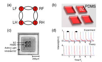
Figure 1: (a) Schematic of a network of a ring of 4 inhibitory coupled oscillators. Indexing of nodes is indicated as either a number (1,2,3,4), or leg of a quadruped (LF, RF, RH, LH) with L left, R right, F front and H hind. (b) Schematic of the experimental system. The reactors are divots in the PDMS, filled with BZ and sealed between 2 glass plates. (c) Photograph of BZ filled 4-ring network. Actinic light illuminates BZ in a channel surrounding the network and provides a constant chemical boundary condition. (d) Two adjacent reactors (red and blue traces) in the network oscillating $180^{\circ}$ out-of-phase with each other. Top: Measured transmitted intensity versus time. Bottom: Simulated oxidized catalyst concentration [mM] versus time. In both, time is rescaled by oscillation period $T_{0}$, indicated by the two arrows.

II Results

II.1 Experimental Reaction-Diffusion Network

We designed a reaction-diffusion network consisting of a ring of four diffusively coupled nanoliter volume batch reactors laid out in a square 2x2 lattice with nearest neighbor coupling (see Fig. 1). Previously, we employed emulsions containing the BZ oscillating reaction to study reaction-diffusion networksToiya et al. (2010); Delgado et al. (2011); Li et al. (2014); Tompkins et al. (2014, 2015); Li et al. (2015); Wang et al. (2016); Norton et al. (2019). But the diffusive coupling between surfactant stabilized emulsion drops was difficult to characterize and manufacturing of the networks was challenging, which contributed to a large degree of variability between experiments. Here, to improve reproducibility we manufactured these reactors to high precision from elastomeric PDMS using soft lithography techniques and filled the reactors with the oscillatory BZ reaction as described previouslyLitschel et al. (2018); Sheehy et al. (2020), illustrated in Fig. 1 and in Appendix Appendix A: Experimental Methods. To obtain a large statistical sample of trajectories we made devices that combined 9 or 16 copies of the 2x2 network Litschel et al. (2018). To optimize homogeneity in the chemical concentrations of each of the reactors, we simultaneously filled the entire set of networks by pipetting a drop of BZ that floods all the reactors before sealing the sets of reactors by clamping the PDMS between two glass plates [Supplementary Material SI Fig. 1-2, SI videos in Litschel et al. (2018)].

The chemical coupling between adjacent reactors arises from the permeation of chemical species through the intervening PDMS wall and mainly consists of bromine-induced inhibition, with a weaker activator coupling, perhaps by bromous acid and the bromine dioxide radical Li et al. (2014); Norton et al. (2019); Li et al. (2015); Litschel et al. (2018); Vanag and Epstein (2009); Tompkins et al. (2014); Torbensen et al. (2017a); Wang et al. (2016); Proskurkin and Vanag (2018); Torbensen et al. (2017b); Delgado et al. (2011); Vanag and Epstein (2011); Toiya et al. (2010). After mixing the BZ reagents, pipetting them onto the PDMS networks, sealing the networks, and placing the sample in the dark for an induction period of 20 minutes, it was observed that all reactors began to oscillate and collectively form spatiotemporal patterns [Fig. 1(d)] Litschel et al. (2018).

The reactors form a closed system and consequently the oscillators have a finite lifetime as the reactants are consumed and waste products accumulate. However, although the amplitude of the chemical oscillations decreases over time, the oscillators maintain a nearly constant period for a duration of order 70 oscillationsSheehy et al. (2020). Based on this long term stability, we assume that the underlying phase dynamics of the individual BZ oscillators remains constant during the duration of the experiment, thus allowing us to study phase relationships between reactors as they evolve over time [Supplementary Material SI Fig. 4, Movies S1-4]. Each 4-ring network is isolated from the environment because the reactors are surrounded by a zone of photosensitive BZ that is held at constant chemical conditions by the application of actinic lightLitschel et al. (2018). We also assume that each chemical reactor is well mixed, ignoring any spatial variation of chemical concentrations, because the size of the reactor is small compared with the length scale of diffusion, e.g. $w<\sqrt{D\tau}$ with $w$ the width of each square reactor ($w=62~{}$$\mathrm{\SIUnitSymbolMicro m}$), $D$, the diffusion constant of each BZ chemical ($D\sim 10^{-9}\mathrm{m}^{2}\mathrm{s}^{-1}$) and $\tau$, the duration of a BZ oscillation ($\tau\sim 300$s).

II.2 Theory and the Role of Symmetry

The fullest description of the dynamics of the 4-ring network that we consider is a reaction-diffusion network model. It focuses on the time dependent concentrations of the well mixed chemicals in each reactor, denoted as $\left(\bar{c}_{1}(t),\bar{c}_{2}(t),\bar{c}_{3}(t),\bar{c}_{4}(t)\right)$, where $\bar{c}_{j}(t)$ is a vector of concentrations in the $j_{\mathrm{th}}$ reactor with indices as in Fig. 1A. Assuming that the reactors are identical, the behaviors are expected to have the same symmetries as a square, e.g. 3 rotations and 4 reflections. Associated with this symmetry group, the H/K theorem predicts invariant manifolds, subspaces in which the dynamics remains confined, that are universal to any ring of 4 oscillators, enumerated in Table 1. Although the theory is more general, we restrict ourselves to the case in which all the nodes are on the same limit cycle, as this corresponds to experiment. With this assumption the H/K theorem guarantees any system of 4 oscillators with square symmetry possesses 8 categories of invariant manifolds, including 4 categories of phase-locked periodic states. These states are therefore efficiently described by considering the phase relationship between pairs of reactors, defined as the fraction of period they are shifted from each other on their common limit cycle.

Invariant manifolds are denoted by a pair of symmetry operations, (H,K). The first symmetry, H, represents an exchange of nodes that results in the same state subject to one or more phase-shifts. The second symmetry, K, indicates symmetries under which the system is unchanged.

Depending on the constraints imposed by H and K, these solutions may either maintain fixed phase relationships among all four nodes resulting in phase-locked solutions, or leave 1- or 2-dimensional freedom on these relationships, as enumerated in Table 1. The 4 categories of phase-locked periodic states are spatiotemporal periodic patterns that correspond to 6 point invariant manifolds in the phase difference space that can be identified with gaits of quadrupeds enumerated in Table 1 and visualized in Fig. 2(b). The first two categories are Pronk in which all the legs advance simultaneously and Trot for which diagonal legs are in phase, and the two diagonal pairs of legs are half a period out of phase. Pace and Bound form one category and we refer to them interchangeably in the remainder of the text. In Pace, legs on each side are in phase and opposite sides out-of-phase, while for Bound, legs on opposite sides are in phase and the front legs out-of-phase with the hind legs. Clockwise (counter clockwise) Rotary Gallop is another category in which the legs advance in a clockwise (counter clockwise) manner with each leg advancing a quarter of a period later than the preceding leg.

The remaining 4 categories correspond to higher dimensional invariant manifolds (lines or planes) that contain trajectories maintaining partial symmetries. Along 1-dimensional linear invariant manifolds, the network can be split into two pairs of reactors, such that within pairs the reactors are in phase or antiphase, while between pairs reactors have an arbitrary phase-shift. Along 2-dimensional manifolds, two nodes oscillate in phase and the other two nodes are at arbitrary phase-shifts. In fact, the 2-dimensional manifolds intersect the 1-dimensional manifolds, and the 1D manifolds intersect the phase-locked 0-dimensional manifolds [Fig. 2(a)]. Heuristically, these higher dimensional manifolds often act as privileged pathways that both guide and structure transient transitions between the phase-locked states. Beyond predicting the existence of these invariants, the H/K theorem neither prescribes their stability nor precludes the existence of others. To address questions of stability and existence of additional manifolds requires a specific model of the oscillators and their connections.

II.3 Chemical Kinetic and Phase Models

To model the reaction-diffusion dynamics of our experiments we use the Vanag-Epstein model of the BZ reaction, which treats the chemical kinetics of 4 BZ chemicals, Br-, HBrO_2, Ferroin, and Br_2, combined with a diffusive coupling term between chemical species in which the coupling strength is fitted from the data. Noting that $\bar{c}_{i}\in\mathbb{R}^{4}$ are the concentrations of these 4 chemicals in reactor $i\in\{1,2,3,4\}$ and $R_{0}:\mathbb{R}^{4}\mapsto\mathbb{R}^{4}$ denotes the Vanag-Epstein BZ model vector field Li et al. (2014); Norton et al. (2019); Li et al. (2015); Litschel et al. (2018); Vanag and Epstein (2009); Tompkins et al. (2014); Torbensen et al. (2017a); Wang et al. (2016); Proskurkin and Vanag (2018); Torbensen et al. (2017b); Delgado et al. (2011); Vanag and Epstein (2011); Toiya et al. (2010), we obtain the equation:

$$\frac{d}{dt}\bar{c}_{i}=\bar{R}_{0}(\bar{c}_{i})+\sum_{j=1}^{4}A_{ij}\mu(\bar{c}_{j}-\bar{c}_{i})$$ (1)

where $\mu\in\mathbb{R}^{4\times 4}$ accounts for the chemical coupling matrix between two adjacent cells, and depends on the permeability of the PDMS for each chemical species and the geometry of the reactors, while $A\in\mathbb{R}^{4\times 4}$ denotes the adjacency matrix between two reactors that is determined by the network topology [Appendix Appendix C: Best Fit Model for details on the model, choice of parameters and fits of free parameters]. This model ignores spatial concentration gradients inside the reactors, effectively treating reactors as points corresponding to nodes of the network. The model also neglects the occurrence of chemical reactions within the PDMS, which acts as a connector that couples adjacent nodes.

Table 1: Symmetry required invariant manifolds for an oscillator network possessing square or Dihedral 4 ($D_{4}$) symmetry. $D_{4}$, all symmetries of a square; $D_{n}^{p}$, reflection across $n$ diagonals; $D_{n}^{s}$, reflection across $n$, vertical or horizontal, axes; $Z_{4}$, $90^{\circ}$ rotation; $Z_{2}$, $180^{\circ}$ rotation; $1$, no operation. The first 4 classes of manifolds are phase-locked states. The column marked “Phase” graphically indicates the spatiotemporal pattern with symbols representing the phase in percentage of the period $T_{0}$, white circle - $0\%$; white/black - $25\%$; black circle - $50\%$; black/white - $75\%$. $T_{0}$ denotes the period of each oscillator in a given invariant manifold and can vary from manifold to manifold. The second 4 classes of manifolds are symmetrically clustered states, related by arbitrary phase shifts $f_{1},f_{2}$, which vary from 0 to 1 as fraction of a period. The graphical representation of nodes in the column “Phase” have solid, striped, or dot motifs. Different motifs are related by an arbitrary phase shift. Similar motifs with opposite background colors are antiphase with each other.

Point invariant manifolds:
Name (H,K)	Phase	$\bar{c}_{1}$	$\bar{c}_{2}$	$\bar{c}_{3}$	$\bar{c}_{4}$
Pronk ${\scriptstyle(D_{4},D_{4})}$		$\bar{c}(t)$	$\bar{c}(t)$	$\bar{c}(t)$	$\bar{c}(t)$
Trot ${\scriptstyle(D_{4},D^{p}_{2})}$		$\bar{c}(t)$	$\bar{c}(t+\frac{T_{0}}{2})$	$\bar{c}(t)$	$\bar{c}(t+\frac{T_{0}}{2})$
Pace ${\scriptstyle(D^{s}_{2},D^{s}_{1})}_{A}$ Bound ${\scriptstyle(D^{s}_{2},D^{s}_{1})}_{B}$		$\bar{c}(t)$ $\bar{c}(t)$	$\bar{c}(t+\frac{T_{0}}{2})$ $\bar{c}(t)$	$\bar{c}(t+\frac{T_{0}}{2})$ $\bar{c}(t+\frac{T_{0}}{2})$	$\bar{c}(t)$ $\bar{c}(t+\frac{T_{0}}{2})$
CW Gallop ${\scriptstyle(Z_{4},1)}_{A}$ CCW Gallop ${\scriptstyle(Z_{4},1)}_{B}$		$\bar{c}(t)$ $\bar{c}(t)$	$\bar{c}(t+\frac{T_{0}}{4})$ $\bar{c}(t-\frac{T_{0}}{4})$	$\bar{c}(t+\frac{T_{0}}{2})$ $\bar{c}(t+\frac{T_{0}}{2})$	$\bar{c}(t-\frac{T_{0}}{4})$ $\bar{c}(t+\frac{T_{0}}{4})$
Linear invariant manifolds:
${\scriptstyle(D^{s}_{1},D^{s}_{1})}_{A}$ ${\scriptstyle(D^{s}_{1},D^{s}_{1})}_{B}$		$\bar{c}(t)$ $\bar{c}(t)$	$\bar{c}(t+f_{1}T_{0})$ $\bar{c}(t)$	$\bar{c}(t+f_{1}T_{0})$ $\bar{c}(t+f_{1}T_{0})$	$\bar{c}(t)$ $\bar{c}(t+f_{1}T_{0})$
${\scriptstyle(D^{s}_{1},1)}_{A}$ ${\scriptstyle(D^{s}_{1},1)}_{B}$		$\bar{c}(t)$ $\bar{c}(t)$	$\bar{c}(t+\frac{T_{0}}{2})$ $\bar{c}(t+(f_{1}+\frac{1}{2})T_{0})$	$\bar{c}(t+f_{1}T_{0})$ $\bar{c}(t+f_{1}T_{0})$	$\bar{c}(t+(f_{1}+\frac{1}{2})T_{0})$ $\bar{c}(t+\frac{1}{2}T_{0})$
${\scriptstyle(Z_{2},1)}$		$\bar{c}(t)$	$\bar{c}(t+f_{1}T_{0})$	$\bar{c}(t+\frac{T_{0}}{2})$	$\bar{c}(t+(f_{1}+\frac{1}{2})T_{0})$
Planar invariant manifolds:
${\scriptstyle(D^{p}_{1},D^{p}_{1})}_{A}$ ${\scriptstyle(D^{p}_{1},D^{p}_{1})}_{B}$		$\bar{c}(t)$ $\bar{c}(t)$	$\bar{c}(t+f_{1}T_{0})$ $\bar{c}(t+f_{1}T_{0})$	$\bar{c}(t)$ $\bar{c}(t+f_{2}T_{0})$	$\bar{c}(t+f_{2}T_{0})$ $\bar{c}(t+f_{1}T_{0})$

Under the assumption that all reactors are oscillating on the same limit cycle, we can parameterize the time dependent concentrations through the phase of that cycle, as proposed by Winfree Winfree (1967) and widely used in various applications Ermentrout and Terman (2009); Kuramoto (1984); Schwemmer and Lewis (2012); Wilson and Ermentrout (2019); Norton et al. (2019); Monga et al. (2019). In this abstraction, the phase variable naturally progresses linearly from $0$ to $2\pi$ at a frequency $\omega_{0}=2\pi/T_{0}$. Perturbing the chemical concentration of an individual reactor will lead to a modification of the phase that depends on the chemical species that is perturbed and phase of the reactor; this function is called the phase response curve (PRC). The impact on the phase of one reactor due to diffusive coupling from a neighbor can be summarized through the interaction function, $H$, derived from convolving the PRC with the diffusive coupling between reactors and averaging over a period Kuramoto (1984) [Appendix Appendix C: Best Fit Model]. Notably, this reduction of the chemical model of Eq. 1 to a phase model introduces no new parameters. Best fits between experiment and model are obtained with the interaction function $H$ that arises from a combination of Br_2 and HBrO_2, as shown in Fig. 6(a). This leads to the phase equation:

$$\frac{d}{dt}\phi_{i}=\omega_{0}+k\sum_{j=1}^{4}A_{ij}H(\phi_{j}-\phi_{i})$$ (2)

where $k$ the diffusive coupling rate.

Noting that the right hand side of Eq.2 depends only on phase difference $\theta_{ij}\equiv\phi_{i}-\phi_{j}$; we therefore arbitrarily choose the three phase differences $\bar{\theta}=(\theta_{21},\theta_{32},\theta_{43})$ as the new system variables and recast the dynamics accordingly,

$$\frac{d}{dt}\bar{\theta}=\bar{\Psi}(\bar{\theta})$$ (3)

with $\bar{\Psi}(\bar{\theta})$ following directly from Eq. 2. As each of the phase differences is periodic on $(0,2\pi]$, the state-space is a 3-torus. Although the 3-torus cannot be drawn in three dimensions, it is equivalent to a Cartesian cube with periodic boundaries, allowing visualization of the full dynamics.

Dynamics in the State-space of Phase Differences

This new coordinate system transforms the invariant manifolds identified by the H/K theorem in Table 1 to simple, geometric objects: points, lines, and planes, enumerated in Table 2. This transformation enables the consequences of the H/K theorem on the dynamics in state-space to be visualized in a way that would be impossible in the full chemical model, Eq. 1. The point invariant manifolds Pronk, Bound, Trot, Rotary Gallop become steady-states in this new frame, rather than high-dimensional limit cycles. We are able to readily classify them as either attractors, repellers or saddles, according to whether the velocity vectors surrounding the steady-state point inward, outward or change sign depending on orientation, respectively Strogatz (1994). Beyond the steady-states in the form of points, Fig. 2A shows a state-space structured by additional invariant manifolds in the form of lines and planes, all required by the spatiotemporal symmetries of the oscillator network.

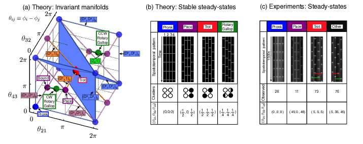
Figure 2: (a) The 8 categories of invariant manifolds for a network of 4 nodes with square symmetry predicted by the H/K theory are presented in the state-space of phase differences. There are 4 categories of phase-locked periodic states (points), 3 categories of lines and 1 category of planes. The state-space is periodic and invariant manifolds that are identical mod $2\pi$ are rendered in translucent colors. (b) (First row) The 4 point manifolds predicted by theory, Pronk, Pace, Trot and Gallop, are represented as space-time plots, (second row) as networks with fixed phase differences and (third row) as a triplet of phase differences, $(\theta_{21},\theta_{32},\theta_{43})$, with units of fraction of a period. (c) (First row) In experiment, 3 of the 4 phase-locked gaits are observed, while Rotary Gallop is never observed. However, a myriad of states with an unclear correspondence to theory are observed, labeled “Other”. The “Other” states are more similar to Trot than Pronk, Pace or Gallop in terms of space-time plots and phase differences. However, Trot and “Other” are qualitatively distinct states because in Trot diagonal nodes oscillate in-phase while in “Other” they oscillate with large phase shifts between them, shown by the red and green bars over the space-time plots. (Second row) The number of times a state is observed is recorded and (Third row) the measured phase difference is listed. Videos of experiments shown in Movies S1-S4.

The dynamical system of Equation [3] predicts that the network is multistable, with the point H/K manifolds forming competing attractors. We simulated exhaustively the model and observed that each initial condition flows to one of the four categories of phase-locked attractor states; (1) Pronk, (2) Pace/Bound, (3) Trot, and (4) CW/CCW Gallop [Fig. 3(a)(b)]. Furthermore, we show in the Supplementary Material SI Sec. IIB that the system predicts the six phase-locked states are linearly stable, and thus attractors.

We found that the theoretical model also possesses many unstable, saddle phase-locked steady-states in addition to the six H/K derived attractors. In fact, topology predicts the existence of unstable steady-states. The topological index of both attractors and saddles with one attracting direction is +1, while the index of both repellors and saddles with two attracting directions is -1. Topology requires that the sum of the topological indices of all the steady-states must equal 0, the Euler characteristic of a 3-torus, as shown in the Supplementary Material SI Sec. IV. Given the six H/K point invariant manifolds are attractors, we conclude there must be at least six unstable steady-states located in the 3-torus to satisfy the required charge neutrality. Moreover, unstable states organize the separatrices between invariant manifolds containing more than one attractor. We numerically searched for the required unstable states and found 158 saddle and 4 unstable steady-states dispersed throughout the state-space shown in Supplementary Material SI Fig. 7. A notable and unexplained fact is that of the 168 numerically identified phase-locked steady-states, the sole attractors are the six invariant point manifolds required by the H/K theorem.

Table 2: Symmetry required invariant manifolds parameterized by relative phase. $f_{1},f_{2}$, which vary from 0 to $2\pi$. All representations, modulo $2\pi$, are shown.

Point invariant manifolds:
Name	Phases	Hyperplane
Pronk		$(\theta_{21}=\theta_{32}=\theta_{43}=0)$
Trot		$(\theta_{21}=\theta_{32}=\theta_{43}=\pi)$
Pace Bound		$(\theta_{21}=-\theta_{43}=\pi,\theta_{32}=0)$ $(\theta_{21}=-\theta_{43}=0,\theta_{32}=\pi)$
CW Gallop CCW Gallop		$(\theta_{21}=\theta_{32}=\theta_{43}=+\frac{\pi}{2})$ $(\theta_{21}=\theta_{32}=\theta_{43}=-\frac{\pi}{2})$
Linear invariant manifolds:
${\scriptstyle(D^{s}_{1},D^{s}_{1})_{A}}$ ${\scriptstyle(D^{s}_{1},D^{s}_{1})_{B}}$		$(\theta_{21}=-\theta_{43}=f_{1},\theta_{32}=0)$ $(\theta_{21}=\theta_{43}=0,\theta_{32}=f_{1})$
${\scriptstyle(D^{s}_{1},1)}_{A}$ ${\scriptstyle(D^{s}_{1},1)}_{B}$		$(\theta_{21}=\pi,\theta_{32}=f_{1},\theta_{43}=-\theta_{32})$ $(\theta_{21}=f_{1},\theta_{32}=\pi,\theta_{43}=\pi)$
${\scriptstyle(Z_{2},1)}$		$(\theta_{21}=f_{1},\theta_{32}=\pi-f_{1},\theta_{43}=f_{1})$
Planar invariant manifolds:
${\scriptstyle(D^{p}_{1},D^{p}_{1})}_{A}$ ${\scriptstyle(D^{p}_{1},D^{p}_{1})}_{B}$		$(\theta_{21}=-\theta_{32},\theta_{32}=f_{1},\theta_{43}=f_{2})$ $(\theta_{21}=f_{1},\theta_{32}=f_{2},\theta_{43}=-\theta_{32})$

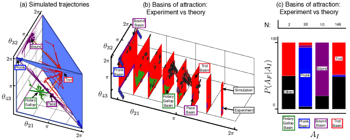
Figure 3: Basins of attraction. States are labeled as in Fig. 2. (a) Simulations of eqn 3 show that all trajectories converge to the H/K point invariant manifolds, Pronk, Bound, Rotary Gallop or Trot, depending on initial condition. Video of different perspectives in 3D are shown in movie S5. The corresponding plot of all experiment is shown in movie S6. (b) Basin of attraction for experiments and theory. The theoretical basins of attraction are colormaps computed from $5399$ simulations, including those in (a). For example, if an initial state is colored red, then it will flow to the Trot attractor. The experimental basins of attraction are partially reconstructed by disks located at their initial condition and colored by the attractor to which they converge, with the color code indicated in (c). We artificially shift slightly the experimental points with nearby initial conditions so that they are revealed. Video of different perspectives in 3D are shown in movie S7. (c) The probability, $P(A_{F}|A_{I})$ , that an experiment which started at a set of phase differences in a given theoretical basin, $A_{I}$, converges to each of the 4 experimental attractors, $A_{F}$. The number of observations is listed in the row labeled “N”. For example, of the 2 initial conditions corresponding to Rotary Gallop, one ended up in the Trot basin and one in the Other basin, but neither went to the predicted basin. In contrast, of the 148 states initially in Trot, 48.7% went to Other, 2.0% to Pronk, 1.3% to Bound and 48.0% to Trot.

We numerically determined the basins of attraction of each attractor by dividing the 3-torus into a fine grid and identifying each initial point with the attractor to which it flowed, as shown in Fig. 3A-B Pusuluri et al. (2020). The Pronk, Bound and Rotary Gallop basins are smooth, closed volumes while the Trot basin fills the rest of the state-space [Fig. 3(b)]. The state with largest basin of attraction is Trot, followed by Rotary Gallop, Bound and Pronk. The attraction basin of the Bound state is anisotropic and aligned with the $(D^{s}_{1},D^{s}_{1})$ invariant manifolds [Fig. 3(a),4(a)]. Fig. 3(a) and 4(b) reveal that trajectories remain near the $(D^{p}_{1},D^{p}_{1})$ invariant manifolds as they flow to Trot. Theory predicts that the network’s trajectories flowing towards its attractors are constrained and shaped by H/K linear and planar invariant manifolds.

To further elucidate how symmetric invariant manifolds guide and structure dynamics, we focus on the transverse dynamics, namely flows perpendicular to the invariant manifolds. We combined the unique system dynamics, Eqns. 2 and 3, and the universal structure of the line and plane invariant manifolds to semi-analytically compute the manifolds’ transverse Lyapunov exponents, which measure the local attraction or repulsion rate of trajectories to or from them Ashwin et al. (1996); Pecora and Carroll (1998); Pecora et al. (2014), in terms of the interaction function, $H$ [Appendix Appendix E: Computing Transverse Lyapunov Exponents of Invariant Manifolds]. The majority of the domains of the $(D^{s}_{1},D^{s}_{1})$ and $(D^{p}_{1},D^{p}_{1})$ manifolds are covered with negative exponents [Fig. 4(c)]. This causes trajectories to collapse and remain on these invariant manifolds [Fig. 4(a)(b)] Pecora et al. (2014). While the regions with negative exponents organize the flows along the invariant manifolds, the small regions of positive exponents contain the separatrices of attractors on the same invariant manifolds, shown as saddles in the Supplementary Material SI Fig. 7. In this way, the theory combines the restrictions of symmetry and the unique system dynamics to predict both the basins of attraction of the attractors and the symmetric, clustered transient transitions along the linear and planar invariant manifolds that connect the attractors.

The higher order H/K invariant manifolds are not the only invariant manifolds controlling transient flows. Additional invariant manifolds arise in the vicinity of steady-states because linear stability analysis permits an eigenvector decomposition of the dynamics. We see such an invariant manifold exists about the Rotary Gallop attractor as all the surrounding trajectories coalesce into a plane [Fig. 3(a)]. This invariant manifold is not aligned with any H/K invariant manifold and arises from the unique system dynamics rather than the H/K theorem or symmetry.

Experimental Observations of Dynamics

To compare the geometric framework provided by the theory of equivariant dynamics with experiment, we defined a reactor’s phase in reference to the moments of maximum oxidation, corresponding to a maximum in transmitted light intensity [Fig. 1(d)]. These moments were attributed phase $2\pi$, and phase was defined as the fraction of time spent between two peaks. This allows us to directly compare theory with experiment by measuring the experimental phase differences between 3 sequential, adjacent pairs of reactors $(\theta_{21},\theta_{32},\theta_{43})$, and to characterize the dynamics relative to invariant manifolds and their stability derived from the model.

We conducted 318 experiments of which 186, or 58%, phase-locked as defined in Appendix Appendix B: Phase-Locked Criteria. During the interval of time soon after the first oscillation and before phase-locking, the oscillation periods of all of the reactors remained similar, $\pm 10\%$. Because the periods of the oscillators are similar, we make the assumption that these reactors are on the same limit cycle. Experiments were stopped either when the system phase-locked or when 70 oscillations occurred, after which the amount of reactants consumed led to the oscillation periods becoming highly variable. We monitored the initial condition, as well as the full transient trajectory for each of the 186 trajectories on their path to phase locking. This allowed the assessment of whether the trajectories were constrained by the invariant manifolds and were affected by the transversal stability, as predicted by theory.

To classify experimental phase-locked states we measure the distance between the observed state and each of the theoretical attractors using a metric appropriate for a 3-torus [Appendix Appendix D: Metric of Distance]. Each phase-locked state is classified as the nearest attractor, or as Other if they are more than 1.0[rad] from each of the H/K attractors. Of the observed steady-states, a majority of $59\%$ correspond to the predicted Pronk, Bound and Trot point invariant manifolds [Fig. 2(c)]. We were initially baffled by the remaining $41\%$ of the observed phase-locked states as they are located a distance from each of the 4 classes of attractors that exceeds the aforementioned threshold radius [Fig. 2(c)], raising the question of their origin as they were not predicted by theory.

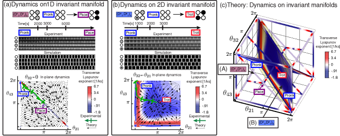
Figure 4: Transient dynamics along higher order H/K invariant manifolds in experiment and simulation. (a) Space-time plots from an experiment and simulation with a near-Pronk initial state transitioning to Pace. States form 2 symmetric clusters corresponding to the $(D^{s}_{1},D^{s}_{1})$ invariant manifold. In the lower panel the experimental trajectory is shown as an arrow traveling through a 2D slice of state-space superimposed over the theoretical velocity field. Video of experiment synchronized to progression along space-time plot and trajectory in state-space shown in movie S8. (b) Space-time plots from an experiment and simulation with a near-Pronk initial state transitioning to Trot. The transition corresponds to the $(D^{p}_{1},D^{p}_{1})$ invariant manifold. Video of experiment synchronized to progression along space-time plot and trajectory in state-space shown in movie S9. (c) The invariant manifold surfaces attract or repulse in a state-dependent manner. The analytically computed transverse Lyapunov exponents [Appendix Appendix E: Computing Transverse Lyapunov Exponents of Invariant Manifolds] are shown via heatmaps. When positive it indicates nearby trajectories are repulsed from the invariant manifold. When negative it indicates attraction. Both the 2D $(D^{p}_{1},D^{p}_{1})$ and 1D $(D^{s}_{1},D^{s}_{1})$ invariant manifolds are largely attracting. Video of 3D perspective of plot in movie S10.

Strikingly, Fig. 4(a)(b) shows that experimental trajectories starting near invariant manifolds $(D^{s}_{1},D^{s}_{1})$ and $(D^{p}_{1},D^{p}_{1})$ closely follow the dynamics predicted by the theory. Such a consistency between experimental observations and clustered transient states predicted on the basis of network symmetry alone is quite remarkable. This suggests that the universal properties dictated solely by the symmetry of the system not only predict stationary behaviors of an experimental system, but also constrain transient dynamics from an initial condition to a stationary state.

There are three other noteworthy comparisons to make between theory and experiment. Firstly, we find experiments and theory have similar shaped Pronk, Bound and Trot basins of attraction, as illustrated in Fig. 3(b)(c). Secondly, the theoretically predicted Trot attractor is symmetrically surrounded by an extended cloud of phase-locked states, denoted Other, which are significantly far from Trot, yet within the predicted Trot basin of attraction. These observations suggest that the experimental Other states are associated with the predicted Trot state, as shown in Fig. 3(b)(c) and Fig. 5(a). Thirdly, the Rotary Gallop states were absent in all our experiments. This is particularly surprising because the theory attributes to that state a large basin of attraction.

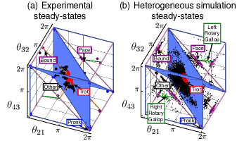
Figure 5: Comparison between experiment and simulation with heterogeneous oscillator frequencies. Phase-locked states are colored by which H/K point manifold they are closest to, or as “Other” if they are more than 1.0 [rad] away from each gait. States are labeled as in Fig. 2. (a) Experiments. (b) Simulations with heterogeneity. A 3% percent coefficient of variation in unperturbed frequencies, $\omega_{i}$, caused a 23-fold reduction in observed Rotary Gallop steady-states compared to the homogeneous simulations in Fig. 3(a)(b). Videos of 3D perspectives of plots shown in movies S11 and S12, respectively.

Inclusion of Slight Heterogeneity in Theory

A hypothesis to account for these discrepancies between theory and experiment is to consider heterogeneities. Indeed, chemical systems differ from theoretical models in that they are bound to be heterogeneous, and in particular imperfectly symmetrical Kuramoto (1984); Strogatz (2001). For instance, modeling BZ micro-oscillators with small degrees of heterogeneity in reactor chemistry (in turn associated with heterogeneous frequencies), or in reactor volume, led in various situations to better match experimental results Tompkins et al. (2014); Norton et al. (2019); Li et al. (2015). We thus tested whether small degrees of heterogeneity between reactors could indeed explain part of the discrepancy between theory and experiments. To this purpose, we defined a variation of our network model including heterogeneities between reactors, which, using phase reduction [see detail in Appendix Appendix C: Best Fit Model] led us to analyze a phase model with heterogeneous frequency of typeSchwemmer and Lewis (2012):

$$\frac{d}{dt}\phi_{i}=\omega_{i}+k\sum_{j=1}^{4}A_{ij}H(\phi_{j}-\phi_{i})$$ (4)

To fit equation 4 to a trajectory of phase differences measured during an experiment requires a specific set of non-zero unperturbed frequency differences $\omega_{i}-\omega_{j}$ [Appendix Appendix C: Best Fit Model]. Although the best fit unperturbed frequencies are different for each experiment, their statistical distribution fits a Laplacian probability distribution function corresponding to unperturbed frequencies $\omega_{i}$ having a percent coefficient of variation of $\pm 3\%$[Supplementary Material SI Sec. II]. Multiple simulations from each initial condition are run using a new sampling from the best fit unperturbed frequency differences probability density function. The steady-state phase differences for phase-locking trajectories observed experimentally and in simulations with heterogeneity are shown in Fig. 5.

With the introduction of heterogeneity in the model using probability distributions fitted to the experiments, we observed that the Rotary Gallop state disappears, just as in experiment [Fig. 5]. The percent of phase-locked states which were Rotary Gallop was high in symmetric simulations in which all oscillators had the same frequency, $6.0\%(N=5,399)$ compared to $0.26\%(N=34,713)$ in heterogeneous simulations and $0\%(N=186)$ in experiments. This 23-fold decrease in percentage of Rotary Gallop steady-states is significantly larger than the 1.5, 2.3 and 3.2-fold decreases for Trot, Bound and Pronk. Further, the Trot, Bound, and Pronk states in simulation are clustered in a manner corresponding to experiment [Fig. 5(b)]. In particular, we observe states, termed Other, that form a large cluster of phase-locked states centered about Trot [Fig. 5]. We therefore conclude that small levels of heterogeneity can indeed account for the main discrepancies between the theory and the models.

Discussion

Symmetry principles have been used to design network topologies of electronic oscillators that generate desired dynamics Matheny et al. (2019); In et al. (2003). The correspondence between theory and experiment was ascribed to the precision of the fabrication process of these electromechanical devices, which possessed intrinsic frequencies with only 0.001% percent variation, ensuring the equivalence of each network node and connection Matheny et al. (2019). While these experiments demonstrated the relevance of equivariant dynamics to experiments, it is unresolved whether the predictions of H/K theorem persist in the biological milieu which never achieve such interchangeability Winfree (1967).

Approaching biological systems directly in a similar manner is difficult because the intrinsic dynamics are both complex and unknown. One study found that oscillatory slime mold confined to networks with specified symmetries support aspects of the H/K theory Takamatsu et al. (2001). The biological oscillators in this system possessed intrinsic frequencies with 10% percent variation Takamatsu et al. (2000). Despite being 4 orders of magnitude more heterogeneous than the electronic system, symmetric dynamics emerged. Still, while these results are intriguing, because the underlying chemical dynamics of slime mold are not fully understood and the total number of oscillations are small, it is impossible to assess the stability of observed spatiotemporal patterns, transient dynamics, or the impact of heterogeneity. Thus, minimally complex reaction-diffusion based systems provide an essential linkage between idealized theory and biology.

Our experiments showed both consistencies and discrepancies with the symmetry-based theory. In particular, most phase-locked states were recovered, and tracking trajectories from an initial condition to a phase-locked state showed that the theory not only predicted the steady-states, but also their basins of attraction and, more surprisingly, transient dynamics and transverse stability along invariant manifolds.

However, through combining theory and experiment on a model system, our results suggest that heterogeneity eliminates some states, but not others, raising the question of understanding which states are the most sensitive to heterogeneity. A natural hypothesis would be that the states disappearing upon addition of heterogeneity would correspond to states which in the absence of heterogeneity, would have weaker stability. Established theory concerning heterogeneity in oscillator networks predicts the impact of heterogeneity is inversely proportional to the system’s linear stability Norton et al. (2019); Skardal et al. (2014). Following this approach, we computed the maximum Lyapunov exponent for each of the phase-locked states. We found that Pronk and Bound have the same maximum Lyapunov exponents, $-2\text{\times}{10}^{-4}$ $[\mathrm{s^{-1}}]$, while Rotary Gallop has a threefold larger value, $-6\text{\times}{10}^{-4}$ $[\mathrm{s^{-1}}]$ [Supplementary Material SI Fig. 6]. In other words, in the absence of heterogeneity, the Rotary Gallop state has a higher magnitude vector field pointing in towards it than the other states. Therefore, interestingly, Rotary Gallop has a stronger stability and a larger basin of attraction relative to Pronk and Bound, and yet appears more sensitive to heterogeneity. This raises the question of characterizing how symmetric states are affected by perturbations, a largely open theoretical question with important applications.

Conclusion

Understanding how network structure controls spatiotemporal pattern formation remains a central problem in network science. Analysis of spatial network symmetries has led to great progress by illuminating mechanisms behind the emergence of clustered, dynamical states. Specifically, tools for identifying group orbits  Pecora et al. (2014) and equitable partitions  Belykh and Hasler (2011); Siddique et al. (2018) have been particularly fruitful in systematizing the identification of topology-required clustered states. Here, the low-dimensionality of the representation of a 4-ring network by phase differences allows us to concretely illustrate complex but universal features of the dynamical landscape underpinning the emergence of clusters.

We showed that a longstanding theoretical conjecture, that symmetry can dictate function in biological systems, can be used to rationally engineer a spontaneously organizing reaction-diffusion network of Belousov-Zhabotinsky oscillators. Thus, our results offer promise for applying symmetry principles as a tool for designing out-of-equilibrium materials and understanding biological dynamics. Contemporary theory Golubitsky et al. (1999); Golubitsky and Stewart (2000b) proves that oscillator networks with the same symmetry as the 4-ring we studied are required to share a universal list of phase-locked states and transient dynamics.

By mapping both the high-dimensional chemical model and experimental observations to a 3D state-space of phase differences, we showed that the symmetry required invariant manifolds take on simple forms. Point manifolds are phase-locked states with spatiotemporal patterns that we recognize as quadruped gaits. The higher dimensional manifolds consist of lines and planes in state-space that guide the transient dynamics from one point manifold to another. Additionally, network sub-clusters are sequentially synchronized when convergence to a final spatiotemporal pattern occurs along these manifolds. Thus the H/K theorem imposes a great deal of structure on the phase-locked and transient dynamics of the system that is dependent only on the network’s topology and independent of any of the specifics of the oscillators and their coupling. These results therefore provide strong support to the hypothesis that symmetries in chemical or biological neural networks organize functional patterns, such as locomotion Golubitsky and Stewart (2000b); Stewart and Golubitsky (2015).

An important aspect of this study is its exhaustiveness: analyzing a small network allowed a complete application of the H/K theorem. In our integrated reaction-diffusion system, the adjustable parameters were few, and the number of oscillations per trial and the number of trials were large, thereby facilitating a detailed comparison between theory and experiment. Having shown the successes and limitations of the theorem using the general methods of phase-reduction, it provides a framework for analyzing other networks. Most readily comparable will be other networks with polygonal geometry. For larger-scale networks, it remains in principle possible to numerically employ a similar methodology to predict spatiotemporal patterns by applying the H/K framework in complex networks, for example by using computer-assisted calculations Pecora et al. (2014). However, for large numbers of nodes and symmetries, it may become more practical and meaningful to approximate the network by a continuum and use continuous symmetry groups (e.g., dense lattices could be approximated by planes, or polygons with a large number of nodes by circles, with continuous rotations or translations as symmetries) Vivancos et al. (1995); Bosking et al. (1997); Bressloff et al. (2001a, b). Moreover, extensions of the theory will allow prediction of further invariant manifolds, which do not arise directly from the symmetry group of the network Golubitsky and Stewart (2006); Schaub et al. (2016); Salova and D’Souza (2020).

These experiments raise for the first time the deep theoretical question of how, in spite of this general consistency between symmetry based theories and experiment, that even small levels of heterogeneity have the potential of crucially modifying the dynamics. Two examples are that heterogeneity renders some symmetry-derived states no longer observable and the surprising phenomenon whereby the sensitivity of states to heterogeneous perturbations does not correlate with the strength and size of the basin of attraction of the state in the ideally symmetric system. These results emphasize the importance of assessing the robustness of symmetry-predicted results in the face of heterogeneity. This assessment is essential to validate the application of the symmetry-based theory to biological systems, as well as to guide the design of chemical reaction-diffusion networks to be used in engineered applications, such as soft robotics.

To date, we know of no theoretical framework addressing the structural stability of H/K’s predictions to heterogeneity that can explain our experimental and numerical observations. Thus, this work encourages more theoretical and experimental studies such as systematically introducing symmetry breaking by controlling the degree to which nodes and connections are distinct, so as to finely characterize the origin of heterogeneity-induced destabilization or vanishing of steady-statesNorton et al. (2019). Our experimental system, used here for the first time to test symmetry based theories in reaction-diffusion networks, is ideally suited for such studiesLitschel et al. (2018). Our results partially reveal the complex role of network structure on dynamics, but to articulate fully the engineering principles of network dynamics it remains to elucidate how heterogeneity impacts performance. We hypothesize that similarly to the phase-locked and transient dynamics studied here, the impact of network heterogeneity is partially symmetry generic and partially model specific.

Appendix A: Experimental Methods

II.4 Network Fabrication

The microfluidic reaction-diffusion network was made out of four adjacent reactors embedded in polydimethylsiloxane (PDMS). The reactors are formed out of divots in PDMS, forming effective buckets, which can be filled and then sealed all together by a piece of glass, forming a common lid. We manufactured these divots using a soft lithographic process in which PDMS is cured while pressed against an inverse (positive) of the divots made out of a photoresist deposited onto a silicon wafer. This was performed as previously published Litschel et al. (2018), with the exception of one adaptation described below. This generates a glass microscope slide coated with many reactors organized into networks of four reactors, shown in Fig. 1(b)(c) and Supplementary Material SI Fig. 1 and 2(a).

The dimensions chosen for the network allow for robust coupling of four nodes in ring topology. By adjusting the sizes and distances between reactors we found that rectangular reactor dimensions 62$\mathrm{\SIUnitSymbolMicro m}$ x 62$\mathrm{\SIUnitSymbolMicro m}$ x 30$\mathrm{\SIUnitSymbolMicro m}$ (L x W x H) with side-to-side distance 26 $\mathrm{\SIUnitSymbolMicro m}$ resulted in strong coupling. The network reactors are organized in a 2 by 2 grid [Fig. 1(b)(c)] in such a way that nearest neighbor reactors possess much more shared surface area relative next-nearest neighbors across the diagonal. This results in a ring-like connectivity, where coupling between nearest neighbors is stronger than across the diagonal. The rectangle of BZ surrounding the network [Fig. 1 (c)] is forced into a steady-state, setting the concentration of chemicals surrounding the network. During each experiment we observe nine or sixteen strongly coupled, individual networks, separated from one another by controlled barriers [Supplementary Material SI Fig. 1(b)(c)].

The only alteration of the procedure in fabricating the PDMS networks published Litschel et al. (2018) was to change the way in which the PDMS was pressed and cured – instead of a 15$\mathrm{kg}$ lead brick applied for 12 hours followed by baking in a 70C oven, we used a thermal press applying 90-113$\mathrm{kg}$ set at 70C for 2.5 hours. This was found to: a) reproducibly keep the size of the layer of PDMS underneath sample less than 2 $\mathrm{\SIUnitSymbolMicro m}$ [Supplementary Material SI Fig. 1(d)] and b) decrease the probability that the silicon wafer breaks per use.

II.5 Sample Holders

In a previous work the PDMS reactors had BZ sealed inside of them and were loaded into a microscope using an acrylic plastic clamp Litschel et al. (2018). This clamp did not control the temperature of the BZ. However, the frequency of BZ oscillations depends on temperature Bánsági et al. (2009).

To maximize experimental reproducibility, we created a clamp that controlled sample temperatures to within 0.1$\mathrm{\SIUnitSymbolCelsius}$. The clamp’s temperature is controlled through a thermistor that measures the temperature of the clamp nearby the sample [Supplementary Material SI Fig. 2], 2 Peltier (TEC) devices [Supplementary Material SI Fig. 2], and PID feedback between them mediated by an Arduino. The sample is robustly driven to the clamp’s temperature because the clamp possesses a large thermal mass relative the sample and large thermal contact area with the sample [Supplementary Material SI Fig. 2]. During all trials samples were kept at $22.0$ $\mathrm{\SIUnitSymbolCelsius}$.

We seal samples in the temperature-controlled clamp exactly the same way as with the previous, plastic clamp Litschel et al. (2018), described in Appendix Appendix A: Experimental Methods Protocol.

II.6 BZ Chemical Preparation

The BZ loaded into the microfluidic network is first mixed outside the microfluidic device. A .24$\mathrm{mL}$ volume of photo-sensitive BZ is prepared by sequentially adding equal $60$$\mathrm{\SIUnitSymbolMicro L}$ volumes of Sulfuric acid, Sodium Bromide, Malonic acid, Sodium Bromate, Ferroin then Tris(2,2’-bipyridyl)dichlororuthenium(II)hexahydrate to an Eppendorf tube, then mixing it with a Vortex mixer. Note that during the sequential pipetting of the chemicals, upon adding the Sodium Bromate, the solution converts from colorless to a vivid, transparent yellow for 15 seconds before returning to a colorless state. The volumes output by the pipette used had a measured percent coefficient of variance of $1.2\%$. The concentrations of the reagents in the final .24$\mathrm{mL}$ mixture, and ultimately in the individual BZ microreactors, are in Table 3.

Table 3: Final experimental chemical conditions in reactors:

Chemical	Molecular Formula	Concentration $\mathrm{m\textsc{m}}$
Sulfuric Acid	H_2SO_4	$80$
Sodium Bromide	NaBr	$25$
Malonic Acid	C_3H_4O_4	$400$
Sodium Bromate	NaBrO_3	$288$
Ferroin	C_36H_24FeN_6O_4S	$3$
Tris(2,2’-bipyridyl) dichlororuthenium(II) hexahydrate	C_30H_24Cl_2N_6Ru. 6H_2O	$1.2$

II.7 Optics

We measured the chemical state of the reactors through measuring their absorbance of green light. Ferroin’s absorbance of green light changes drastically between its oxidized and reduced state. The green light is filtered to $515\pm 10$$\mathrm{nm}$, to avoid exciting the photocatalyst, Ru(bipy)_3.

Light perturbation, used to set boundary conditions and initial conditions were set by projection of patterned blue light onto the sample, selectively exciting the photocatalyst. As in previous works Litschel et al. (2018); Tompkins et al. (2014); Delgado et al. (2011), the patterned blue light was periodically turned off and on at a high frequency to allow accurate measurement of absorbance of Ferroin, with period $2$ seconds and duty cycle of 50$\%$. During some of the experiments the blue light was homogenized by directly replacing the sample with a CCD and using feedback between projected signals and the measured values to minimize measured variability, as previous published Sheehy et al. (2020).

Boundary conditions were applied by shining light on the rectangle surrounding the network at an intensity that completely inhibit oscillations in it.

Initial conditions were set by applying light to the reactors by inhibiting all reactors with light for 300-600 seconds. Then, the light was turned off at different times from each of the reactors, thus causing them to resume oscillating at different times. The success rate of hitting target initial conditions far from Trot or Pronk was low.

The light intensity of sample illumination was measured by placing a power meter in the sample plane, the results are similar to in previous Delgado et al. (2011) work: Intensity of blue light applied to boundaries: $0.3\pm.04$ $\mathrm{mW}\text{\,}{\mathrm{cm}}^{-2}$, Intensity of blue light applied to reactors during initial condition setting: $1\pm 0.2$$\mathrm{mW}\text{\,}{\mathrm{cm}}^{-2}$, Intensity of blue applied light when projector blank/black: $0.09\pm 0.009$$\mathrm{mW}\text{\,}{\mathrm{cm}}^{-2}$, Intensity of 515nm green sample illumination: $\sim$0.1$\mathrm{mW}\text{\,}{\mathrm{cm}}^{-2}$. Errors, in standard deviations, express variance in average illumination across the whole sample field of view across all experiments, not the variance across the field of view in individual experiments

II.8 Protocol

The protocol for an experiment is as follows:

1. PDMS chip, reentrant window, and O-ring [Supplementary Material SI Fig. 2(a)] are cleaned with isopropyl alcohol, deionized water, and dried with compressed air. They are left under petri dishes to prevent dust accumulation.

2. A small batch of BZ solution is prepared as detailed earlier in Appendix Appendix A: Experimental Methods. Solution is left in a dark chamber.

3. The PDMS chip is plasma treated for 3 minutes at 400$\mathrm{mbar}$ in ambient atmosphere.

4. The BZ solution is then pipetted into the networks of interest in the PDMS chip as shown in depth in supplementary movie S7 of Litschel et al. (2018).

5. Now, with the reentrant window placed approximately above a feature of networks covered by BZ, the reentrant window must be secured more firmly and precisely. While viewing the sample using a stereomicroscope with green filtered transmission illumination, the thumbscrews [Supplementary Material SI Fig. 2] are slowly turned, clamping the device. We alternated tightening them in a zig-zag pattern, with each tightening of a screw being roughly a 1/8 or less rotation. During this process any bubbles which are present in the reactors should decrease in size until they are invisible. Once all reactors are surrounded by dark outlines Supplementary Material SI Fig. 1(a), there are no shearing distortions to the network, and there are no bubbles, this process is halted.

6. The clamp and the network with BZ sealed into it are then left in a dark, room temperature chamber until it has been 40 minute since the BZ was initially mixed in step 2, typically 20 minutes.

7. The clamp is then loaded into the projection illumination microscope Supplementary Material SI Fig. 3(c). Then, a MATLAB code with GUI is used to align a projected pattern onto the sample Supplementary Material SI Fig. 3(b) and initiate temperature control.

8. Light is projected onto boundaries and sets initial conditions of networks as described earlier in Appendix Appendix A: Experimental Methods. Data is gathered for between 3000 and 24000$\mathrm{s}$, $\sim$ 10 and 81 periods of oscillation of each reactor.

9. In a few experiments a second attempt at setting initial conditions was made.

Appendix B: Phase-Locked Criteria

To identify phase-locked states in experiments we require that $\frac{d}{dt}(\phi_{i}-\phi_{j})$ is almost zero and is not accelerating, $\frac{d^{2}}{dt^{2}}(\phi_{i}-\phi_{j})$ is also small. The algorithm used:

1. Calculate the three phase differences versus time: $(\theta_{21},\theta_{32},\theta_{43})$

2. Lowpass them to form: $(\overline{\theta_{21}},\overline{\theta_{32}},\overline{\theta_{43}})$

3. Find the longest region in the $(\overline{\theta_{21}},\overline{\theta_{32}},\overline{\theta_{43}})$ time series when their velocities at below as threshold:

   $$|\frac{d}{dt}\overline{\theta_{21}}|,|\frac{d}{dt}\overline{\theta_{32}}|,|\frac{d}{dt}\overline{\theta_{43}}|<2.5\times 10^{-4}\left[\frac{\text{rad}}{\text{s}}\right]$$

   and the average acceleration is also below a threshold:

   $$\frac{d}{dt}\frac{1}{3}(|\frac{d}{dt}\overline{\theta_{21}}|+|\frac{d}{dt}\overline{\theta_{32}}|+|\frac{d}{dt}\overline{\theta_{43}}|)<9\times 10^{-8}\left[\frac{\text{rad}}{\text{s}^{2}}\right]$$

4. If the longest region is 5 or more periods of oscillation of all oscillators (1500 seconds), we consider the experiment to be phase-locked.

Appendix C: Best Fit Model

II.9 Physical Models of BZ Microoscillators

The chemical concentration oscillations of an isolated BZ microreactor are accurately modeled by the reaction kinetics derived for macroscopic reactors Vanag and Epstein (2009); Sheehy et al. (2020). Denoting concentrations, $\bar{c}=(x,y,z,u)$ where $x=$[HBrO_2], $y=$[Br-], $z=$[Oxidized catalyst], $u=$[Br_2]:

$$\frac{d}{dt}\bar{c}=\bar{R}(\bar{c})$$ (5)

$$\bar{R}(\begin{bmatrix}x\\ y\\ z\\ u\end{bmatrix})=\begin{bmatrix}R_{x}(x,y,z)\\ R_{y}(x,y,z,u)\\ R_{z}(x,z)\\ R_{u}(x,y,u)\end{bmatrix}$$

$$R_{x}(x,y,z)=k_{2}y-k_{1}xy-2k_{3}x^{2}+\frac{k_{4}x(c_{o}-z)}{(c_{o}-z+c_{min})}$$

$$R_{y}(x,y,z)=-2k_{2}y+k_{7}u+k_{9}z-3k_{1}xy-k_{3}x^{2}$$

$$+\frac{k_{I}(c_{o}-z)}{(\frac{b_{C}}{b}+1)}$$

$$R_{z}(x,z)=-(k_{9}+k_{10})z+2\frac{k_{4}x(c_{o}-z)}{(c_{o}-z+c_{min})}+\frac{k_{I}(c_{o}-z)}{(\frac{b_{C}}{b}+1)}$$

$$R_{u}(x,y,u)=k_{2}y-k_{7}u+2k_{1}xy+k_{3}x^{2}$$

Table 4: Simulation parameters known:

Reagent concentrations:
	Description	Value	Unit
$a$	Bromate	$288$	$\mathrm{m\textsc{m}}$
$m$	Malonic acid	$400$	$\mathrm{m\textsc{m}}$
$c_{o}$	Total metal ion catalyst	$4.2$	$\mathrm{m\textsc{m}}$
$h$	Protons	$160$	$\mathrm{m}\mathrm{\textsc{m}}$
$b$	Bromomalonic acid	$0.12*m$	$\mathrm{m\textsc{m}}$
Reagent rates and relevant constants:
		Value	Unit
$k_{1}$		$2\text{\times}{10}^{6}$$h$	${\mathrm{\textsc{m}}}^{-1}\text{\,}{\mathrm{s}}^{-1}$
$k_{2}$		$2h^{2}a$	${\mathrm{s}}^{-1}$
$k_{3}$		$3\text{\times}{10}^{3}$	${\mathrm{\textsc{m}}}^{-1}\text{\,}{\mathrm{s}}^{-1}$
$k_{4}$		$42ha$	${\mathrm{s}}^{-1}$
$k_{5}$		$$5\text{\times}{10}^{9}$h$	${\mathrm{\textsc{m}}}^{-1}\text{\,}{\mathrm{s}}^{-1}$
$k_{6}$		$10$	${\mathrm{s}}^{-1}$
$k_{7}$		$29m$	${\mathrm{s}}^{-1}$
$k_{8}$		$9.3m$	${\mathrm{s}}^{-1}$
$k_{9}$		$b$	${\mathrm{s}}^{-1}$
$k_{10}$		$0.05m$	${\mathrm{s}}^{-1}$
$k_{r}$		$2\text{\times}{10}^{8}$	${\mathrm{\textsc{m}}}^{-1}\text{\,}{\mathrm{s}}^{-1}$
$k_{red}$		$5\text{\times}{10}^{6}$	${\mathrm{\textsc{m}}}^{-1}\text{\,}{\mathrm{s}}^{-1}$
$k_{I}$		$0$	${\mathrm{s}}^{-1}$
$b_{C}$		$0.05$	$\mathrm{\textsc{m}}$
$c_{min}$		$\sqrt{2k_{r}(k_{9}+k_{10})c_{o}/k_{red}^{2}}$	$\mathrm{\textsc{m}}$

The exchange of chemicals between adjacent BZ microreactors is limited because the PDMS between them is apolar. Br_2 is the only apolar intermediate of the BZ reaction which is certainly soluble in and diffusing through the PDMS between reactors. HBrO_2 may also be soluble to a lesser degree Tompkins et al. (2014); Li et al. (2014); Torbensen et al. (2017a, a). Because of the short separations between reactors $\mathcal{O}(10\mu m)$, the diffusion of these chemicals between reactors is assumed to be quasi-static Toiya et al. (2010); Norton et al. (2019). This results in a simple form of linear difference coupling between a pair of BZ microreactors, where $k$ is the diffusive coupling rate of Br_2 and $k_{e}$ is the ratio of the diffusive coupling rate of HBrO_2 relative Br_2:

$$\frac{d}{dt}\bar{c}_{1}=\bar{R}(\bar{c}_{1})+\mu(\bar{c}_{2}-\bar{c}_{1})$$

$$\frac{d}{dt}\bar{c}_{2}=\bar{R}(\bar{c}_{2})+\mu(\bar{c}_{1}-\bar{c}_{2})$$

$$\mu=\begin{bmatrix}k_{e}k&0&0&0\\ 0&0&0&0\\ 0&0&0&0\\ 0&0&0&k\end{bmatrix}$$

To simulate our results, we adapt the above, established model. Firstly, we model the ring-like topology by adding strong diffusive coupling between nearest neighbors and weaker coupling coupling across the diagonal. Secondly, we also permit a small degree of heterogeneity in reaction rates within the reactors, representing: i) differences in reagent concentrations, ii) differences in powers of light hitting photo-sensitive reactors, and iii) slightly different boundary conditions. The model is then a function of: a) $k$, the diffusive coupling rate of Br_2, b) $k_{e}$, the ratio of the coupling rate of HBrO_2 relative Br_2 c) $f$, the ratio of diagonal to nearest neighbor coupling, d) differences in local reactor reaction rates:

$$\frac{d}{dt}\bar{c}_{i}=\bar{R}_{o}(\bar{c}_{i})+\epsilon\bar{r}_{i}(\bar{c}_{i})+\sum_{j\neq i}^{4}A_{ij}\mu(\bar{c}_{j}-\bar{c}_{i})$$ (6)

$$A_{ij}=\begin{bmatrix}0&1&f&1\\ 1&0&1&f\\ f&1&0&1\\ 1&f&0&0\\ \end{bmatrix};\mu=\begin{bmatrix}k_{e}k&0&0&0\\ 0&0&0&0\\ 0&0&0&0\\ 0&0&0&k\\ \end{bmatrix};$$

To ease comparison to experiments and qualitatively understand the role of free parameters, we use established methods Schwemmer and Lewis (2012); Ermentrout and Terman (2009); Wilson and Ermentrout (2019), described later in this section, to reduce the model above Eqn. 6 to the phase model Eqn. 4. The reduced model Eqn. 4 predicts the phase dynamics of the reactors relative one another as a function of the parameters: a) $k$ which scales the interaction function $H$, b) $k_{e}$ which determines the shape of the $H$ function Fig. 6(a), c) $f$ which changes the adjacency matrix, d) differences in local reactors which change intrinsic frequencies $\omega_{i}$.

We then construct a 3D model of the evolution of phase-differences between adjacent nodes in the network. Letting $\theta_{ij}\equiv\phi_{i}-\phi_{j}$ and $\Delta\omega_{ij}\equiv\omega_{i}-\omega_{j}$

$$\frac{d}{dt}\theta_{ij}=\Delta\omega_{ij}+k\biggl{[}\sum_{k\neq i}^{4}A_{ik}H(\phi_{k}-\phi_{i})$$

$$-\sum_{k\neq j}^{4}A_{jk}H(\phi_{k}-\phi_{j})\biggr{]}$$ (7)

$$\frac{d}{dt}\bar{\theta}=\begin{bmatrix}\frac{d}{dt}\theta_{21}\\ \frac{d}{dt}\theta_{32}\\ \frac{d}{dt}\theta_{43}\\ \end{bmatrix}=\bar{\Psi}(\bar{\theta})$$ (9)

This gives us a model which is expected to qualitatively capture the dynamics of the system and allow us to better understand it. Since the parameters of the model, $f$, $k$ and so on, cannot be independently measured, the model must be empirically fit to experimental data. However, the best fit model reveals important, nontrivial insights into our particular symmetric 4 node network and BZ microoscillator networks in general.

The $H$ function is shown in Fig. 6(a). We ran simulations with the $H$ function saved as a Chebychev function Driscoll et al. (2014) using MATLAB’s ODE45 with relative and absolute tolerances of $1\text{\times}{10}^{-10}$.

II.10 Fitting to Experiments

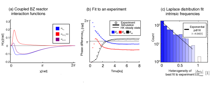
Figure 6: (a) The interaction functions of coupled BZ oscillators. $H_{\text{Br}_{2}}$ is the interaction functions of purely Br_2 coupled reactors. $H_{\text{HBrO}_{2}}$ is the interaction functions of purely HBrO_2 coupled reactor. In the model of our 4 node network Eqn. 9, when $k_{e}$ is not zero the interaction function is $H(\chi)=H_{\text{Br}_{2}}(\chi)+k_{e}H_{\text{HBrO}_{2}}(\chi)$. Since $H_{\text{HBrO}_{2}}$ is largely 0 except for $\chi$ between $0$ and $\pi/2$, $k_{e}$ adds a bump of phase advance near $0$, without affecting the otherwise phase delaying dynamics due to Br_2. $H_{\text{Best fit}}$ corresponds to the interaction function which best fits experiments $k_{e}=0.05$. (b) Example experimental trajectory converging to steady-state (circles), and best fit phase model (solid line). The fit model required slight heterogeneity $\Delta\omega_{ij}\neq 0$. The steady-state phase difference $(\pi,\pi,\pi)$ of the phase model, without best fit heterogeneity, at dashed horizontal line. This is the H/K predicted point invariant manifold nearest to the experimental trajectory. (c) Distribution of best fit nondimensionalized intrinsic frequency differences. They are nondimensionalized by dividing them by best fit coupling rate $k$ times the amplitude of the interaction function $H$, $H_{max}$.

The model Eqn. 9 was fitted to each experimental time series of phase differences versus time [Fig. 6(b)] using nonlinear regression. The nonlinear regression was performed on each individual experiment by constraining a simulation to start from an experimental initial condition, then optimizing the simulation’s parameters to reduce the squared error between its trajectory and the experiment’s trajectory using matlab 2019b’s surrogate optimization. Specifically, the initial condition of phase difference of an experiment was set to be the phase differences when the reactors meet the similar frequency threshold defined in Appendix Appendix A: Experimental Methods, shown in Supplementary Material SI Fig. 4(a)(b). The final point in an experimental trajectory used in a fitting was half way between when the phase-locked condition was met and when it was lost [Supplementary Material SI Fig. 4(a)(c)] or the end of the experiment if it did not unlock.

The identified best fit parameters were: $\Delta\omega_{ij}\neq 0,k=1.8\times 10^{-2}\pm 2.7\times 10^{-3}$ [${\mathrm{s}}^{-1}$], $f=0$[1] and $k_{e}=.05$[1]. The intrinsic frequency differences $\Delta\omega_{ij}$ obeyed a Laplacian distribution $\rho(\Delta\omega_{ij})=\frac{1}{2b}\exp(-\frac{|\Delta\omega_{ij}-\mu|}{b})$ [Fig. 6(c)]. The Laplacian distribution of intrinsic frequencies has a mean, $\mu$, of 0 and rate parameter, $b$, of $2\pi 7\times 10^{-5}$[$\mathrm{rad}\text{\,}{\mathrm{s}}^{-1}$]. Further, the fitting required some excitatory coupling $k_{e}=.05[1]$ and no diagonal coupling $f=0[1]$. The best fit values and the values used in simulations shown in Table 5.

Table 5: Simulation parameters fitted: In ’Fit values’ and ’Values used in theory’ a single number represents the number fit or used in simulations. If in a fit or simulation values were randomly distributed, the form of the distribution is described by ’G’ or ’L’. ’G($\mu,\sigma$)’ represents a Gaussian probability density function with mean $\mu$ and standard deviation $\sigma$. A ’L($\mu,b$)’ represents a Laplacian probability density function with mean $\mu$ and rate parameter $b$.

Parameter	Fit values	Values used in theory	Unit
Coupling:
$k$	G$(1.8\times 10^{-2},2.7\times 10^{-3})$	$2\times 10^{-2}$	${\mathrm{s}}^{-1}$
$k_{e}$	0.05	0.05	1
$f$	0	0	1
Chemical heterogeneity:
$\Delta\omega_{ij}$	L$(0,2\pi 7\times 10^{-5})$	L$(0,2\pi 8\times 10^{-5})$	$\mathrm{rad}\text{\,}{\mathrm{s}}^{-1}$

For a discussion of the values of these parameters measured in previous works and their possible physical relevance, please see Supplementary Material SI Sec. II.

II.11 Best Fit Simulations with Heterogeneity

To determine the impact of experimentally realistic heterogeneity on the model, we ran simulations of Eqn. 4 with the experimental best fit parameters in Table 5. Specifically, heterogeneity in intrinsic frequencies in simulations $\Delta\omega_{ij}$ were drawn from the distribution which fits experiments, a Laplacian distribution defined in Table 5, with mean 0 and rate parameter $2\pi$$8\text{\times}{10}^{-5}$[$\mathrm{rad}\text{\,}{\mathrm{s}}^{-1}$], while all other parameters are the exact, constant value enumerated in the third row of Table 5.

In running simulations from a dense set of initial conditions, each initial condition had 7 simulations initialized from it with independent resamplings of frequency heterogeneity. We thus could observe the impact of heterogeneity throughout state-space by sampling the distribution of heterogeneity in all regions of state-space. The result of 34,713 such simulations are shown in Fig. 5(b).

II.12 Computing Phase Model Reduction

We use established methods Schwemmer and Lewis (2012); Wilson and Ermentrout (2019); Ermentrout and Terman (2009) to reduce the reaction-diffusion model of our 4 reactor network Eqn. 6 to the phase model Eqn. 4. In this framework, we first determine the phase-dependent phase shift of an uncoupled BZ reactor induced by sudden, small additions of its chemical species. We then compute the fluxes of chemical species between a pair of diffusively coupled reactors as a function of their relative phases. By combining these, we determine the rate of phase shift of a reactor as a function of its phase difference with a neighbor.

If chemicals are added to a BZ reactor on its limit cycle, the time until it next spikes will be changed. These time shifts, or phase shifts, depend on amount of chemicals added as well as the time along a period of oscillation, or phase, they are added at. We quantify the phase shifts of an uncoupled reactor to a perturbation at a given phase in terms of phase response curves (PRC). The PRC, $Q$, is a set of curves of phase shift, $\Delta\phi$, as a function of a chemical perturbation’s chemical concentration, $\Delta\bar{c}$, and the phase, $\phi$, at which it is added at. Specifically, it allows calculation of $\Delta\phi=Q(\phi).\Delta\bar{c}$. the case of the 4D model of a BZ reaction 5, $Q:\mathbb{R}^{4}\mapsto\mathbb{S}^{1}$ is a set of 4 curves with units of phase per chemical concentrations [$\mathrm{rad}\text{\,}{\mathrm{\textsc{m}}}^{-1}$]. We compute $Q$ in the limit of infinitesimal perturbations $|\Delta\bar{c}|\to 0$ by the adjoint method Schwemmer and Lewis (2012); Wilson and Ermentrout (2019); Ermentrout and Terman (2009). This allows us to interpret $Q$ as the total derivative $Q(\phi)=\nabla_{\bar{c}}\phi$.

Noting that rate of change of phase of a reactor is $\frac{d}{dt}\phi_{i}$ and is a sum of constant term, its intrinsic frequency $\omega_{i}$, and a time-varying term due to its coupling with its neighbors depending on their relative phases:

$$\frac{d}{dt}\phi_{i}=\omega_{i}+\sum_{j}A_{ij}F(\phi_{i},\phi_{j})$$

Using the PRC we can then compute the rate of change of phase of a reactor $F$ [$\mathrm{rad}\text{\,}{\mathrm{s}}^{-1}$] with respect to an incident, relative phase dependent flux due to coupling $\bar{g}(\phi_{i},\phi_{j})$ [$\mathrm{\textsc{m}}\text{\,}{\mathrm{s}}^{-1}$] using the PRC and the chain rule:

$$F(\phi_{i},\phi_{j})=Q(\phi)\bar{g}(\phi_{i},\phi_{j})\approx\nabla_{\bar{c}}\phi\bar{g}(\phi_{i},\phi_{j})$$ (10)

Letting the unperturbed limit cycle of a BZ reactor be parametrized $\bar{c}_{LC}(\phi)$ and denoting the neighboring reactor $j$, we see from our diffusive coupling Eqn. 6 that the specific form of phase dependent flux neighbors experience $\bar{g}(\phi_{i},\phi_{j})=\mu\left[\bar{c}_{LC}(\phi_{j})-\bar{c}_{LC}(\phi_{i})\right]$ and it follows that:

$$F(\phi_{i},\phi_{j})=Q(\phi)\mu\left[\bar{c}_{LC}(\phi_{j})-\bar{c}_{LC}(\phi_{i})\right]$$ (11)

Note that $F$ is a linear combination of flux due to Br_2, $u$, and HBrO_2, $x$:

$$F(\phi_{i},\phi_{j})=k[Q_{u}(u_{LC}(\phi_{j})-u_{LC}(\phi_{i}))$$

$$+k_{e}Q_{x}(x_{LC}(\phi_{j})-x_{LC}(\phi_{i}))]$$

Since the change of relative phase differences is small during a period of reactor oscillation, we compute $F(\phi_{j},\phi_{i})$ averaged over a cycle Schwemmer and Lewis (2012); Wilson and Ermentrout (2019); Ermentrout and Terman (2009). Doing so transforms it into a function of relative phase difference $H(\phi_{j}-\phi_{i})$. Since $F$ is scaled by $k$, we define $H$ such that it must be used by explicit scaling by $k$, the diffusive coupling rate of Br_2 [$\mathrm{s}$^-1] in eqn 4:

$$H(\phi_{j}-\phi_{i})\equiv k^{-1}(2\pi)^{-1}\int_{0}^{2\pi}F(\alpha,\alpha+\phi_{j}-\phi_{i})d\alpha$$ (13)

We express the interaction function $H$ as the sum of two distinct, separately calculable terms, because $F$ is a linear combination of two functions, one for Br_2 and one for HBrO_2:

$$H(\phi_{j}-\phi_{i})=H_{\ce{Br_{2}}}(\phi_{j}-\phi_{i})+k_{e}H_{\ce{HBrO_{2}}}(\phi_{j}-\phi_{i})$$ (14)

Appendix D: Metric of Distance

To measure distances between two points in the state-space of the 3D phase difference dynamics, both experimentally and in simulations, we found a surprising function $d(\bar{\theta},\bar{\theta}^{\prime})$ was required. For a given pair of points $\bar{\theta}$ and $\bar{\theta}^{\prime}$ $d$ is calculated by the following algorithm:

1. Consider two points in the state-space: $\bar{\theta}^{\prime}=(\theta_{21}^{\prime},\theta_{32}^{\prime},\theta_{43}^{\prime})\text{ and }\bar{\theta}=(\theta_{21},\theta_{32},\theta_{43})$

2. Compute phase difference of fourth edge, which is completely determined by the other three $\bar{\theta}^{\prime}_{f}=(\theta_{21}^{\prime},\theta_{32}^{\prime},\theta_{43}^{\prime},\theta_{21}^{\prime}+\theta_{32}^{\prime}+\theta_{43}^{\prime})=(\theta_{21}^{\prime},\theta_{32}^{\prime},\theta_{43}^{\prime},\theta_{41}^{\prime})\text{ and }\bar{\theta}_{f}=(\theta_{21},\theta_{32},\theta_{43},\theta_{41})$

3. Define a vector of phase difference between states with $\angle$ being complex, or phasor, angle $\theta_{diff_{j}}=\angle\exp(i*(\theta^{\prime}_{f_{j}}-\theta_{f_{j}}))$

4. Let the distance between $\bar{\theta}^{\prime}$ and $\bar{\theta}$ be the Euclidean norm of the 4D phase difference vector $d(\bar{\theta},\bar{\theta}^{\prime})=|\bar{\theta}_{diff}|_{2}$

Appendix E: Computing Transverse Lyapunov Exponents of Invariant Manifolds

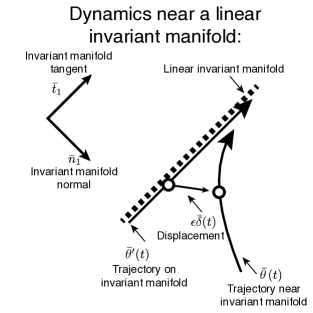
Figure 7: Diagram of flows nearby a linear invariant manifold. Two example trajectories $\bar{\theta}^{\prime}$ and $\bar{\theta}$, which are flows in the state-space of Eqn. 9. Note that because $\bar{\theta}^{\prime}$ is on an invariant manifold, it must continue flowing tangent the invariant manifold indefinitely. However, the trajectory near the invariant manifold $\bar{\theta}$ is not limited in this way. We can consider the displacement between these two trajectories as a function of time $\epsilon\bar{\delta}(t)$. In the case shown, the displacement is shrinking, indicating that the nonlinear flow about the linear invariant manifold near $\bar{\theta}^{\prime}$ is converging towards it. To quantify this behavior more broadly, we utilize he fact the normal component of the displacement will take on a form $\bar{n}_{1}^{T}\epsilon\bar{\delta}(t)\propto\exp(\lambda t)$. The exponential scale $\lambda$, called the transverse Lyapunov exponent, when negative indicates attraction, when positive repulsion.

The maximum transverse Lyapunov exponent (MTLE) of the higher order invariant manifolds describe whether trajectories collapse or diverge from them. If a higher order invariant manifold has a negative MTLE, trajectories will converge towards it Ashwin et al. (1996). In our particular system, we found the MTLE were often easy to calculate and easy to qualitatively understand.

The MTLE of the invariant manifolds can be computed at the phase model level using the well known method of linearizing the dynamics Eqn. 9 about the invariant manifolds Ashwin et al. (1996); Pecora and Carroll (1998); Belykh et al. (2002); Russo and Slotine (2011); Pecora et al. (2014). We explicitly list how we performed this procedure in our case in which the invariant manifolds are linear hyperplanes.

We begin by considering whether a point $\bar{\theta}^{\prime}$ perturbed off an invariant manifold, displaced by $\epsilon\bar{\delta}$ from point $\bar{\theta}^{\prime}$, converges back to or diverges from the manifold [Fig. 7]. The dynamics of the perturbed point take on a simple form:

$$\frac{d}{dt}\bar{\theta}=\bar{\Psi}(\bar{\theta})=\bar{\Psi}(\bar{\theta}^{\prime}+\epsilon\bar{\delta})$$

$$=\bar{\Psi}(\bar{\theta}^{\prime})+\epsilon\nabla_{\bar{x}}\bar{\Psi}(\bar{x})|_{\bar{x}=\bar{\theta}^{\prime}}\bar{\delta}+\mathbb{O}(\epsilon^{2})$$ (15)

It is convenient to consider the displacement between the perturbed solution and the solution on the invariant manifold:

$$\frac{d}{dt}\bar{\delta}=\frac{d}{dt}\bar{\theta}-\frac{d}{dt}\bar{\theta}^{\prime}=\bar{\Psi}(\bar{\theta})-\bar{\Psi}(\bar{\theta}^{\prime})$$

$$=\epsilon\nabla_{\bar{x}}\bar{\Psi}(\bar{x})|_{\bar{x}=\bar{\theta}^{\prime}}\bar{\delta}+\mathbb{O}(\epsilon^{2})$$ (16)

We can determine if the component of the perturbation along a given direction normal to the invariant manifold, $\bar{n}$, grows or decays of the displacement off of the invariant manifold. Letting $J(\bar{x}^{\prime})\equiv\nabla_{\bar{x}}\bar{\Psi}(\bar{x})|_{\bar{x}=\bar{x}^{\prime}}$, the rate of change of the normal distance, $\bar{n}^{T}\bar{\delta}$ is given by:

$$\frac{d}{dt}(\bar{n}^{T}\bar{\delta})\approx\bar{n}^{T}\epsilon J(\bar{\theta}^{\prime})\bar{\delta}$$ (17)

To precisely determine the exponential timescale with which the normal components of the perturbed trajectory grows or shrinks, we use a unitary transformation matrix $P$ to projects a vector of phase differences from the canonical basis into a basis aligned with a given invariant manifold: Letting $\bar{t}_{i}$ be tangent the invariant manifold and $\bar{n}_{i}$ be perpendicular, $P=\left[\bar{t}_{1}...\bar{n}_{1}...\right]^{T}$ s.t. if $\bar{\theta}=c_{t1}\bar{t}_{1}+c_{t2}\bar{t}_{2}...+c_{n_{1}}\bar{n}_{1}+..$. then $P.\bar{\theta}=(c_{t1},c_{t2},...c_{n1}...)$.

Crucially, points on the invariant manifold have no normal components $\forall_{j}c_{nj}=0$ thus $P.\bar{\theta}^{\prime}=(c_{t1},c_{t2},...0,..)$. Similarly, on the invariant manifold the velocity field $P.\bar{\Psi}(\bar{\theta}^{\prime})=\frac{d}{dt}(c_{t1},...c_{n1},...)$ must have all its normal component be 0, $\forall j\frac{d}{dt}c_{nj}=0$, as by definition trajectories cannot flow out of, or transverse, an invariant manifold Fig. 7.

We can now consider the growth or decay of perturbations in or out of a manifold. Let $\bar{\xi}=P.\bar{\delta}$:

$$\frac{d}{dt}\bar{\xi}=\frac{d}{dt}(P.\bar{\delta})=PJ\bar{\delta}=PJP^{-1}\bar{\xi}$$ (18)

Letting $J^{\prime}=PJP^{-1}$: $\frac{d}{dt}\bar{\xi}=J^{\prime}\bar{\xi}$ - a linear time-varying equation. Since the dynamics of the system $\bar{\xi}$ normal to the invariant manifold are all 0, independent on the location along the manifold spanned by the tangent, it follows that the block dynamics in $J^{\prime}$ corresponding to normal components will be independent of those for tangent components Ashwin et al. (1996). The maximum real eigenvalue of this block of normal dynamics gives an approximate bound on the exponential growth or decay of the trajectory’s distance normal an invariant manifold and is called the maximum transverse Lyapunov exponent.

II.13 Algorithm

The algorithm, detailed at length above, is as follows:

1. Choose an invariant manifold $M$, of dimension $k$, in an $n$ node network.

2. Determine $k$ orthonormal vectors which span $M$ and label them the tangent vectors $T$. Determine a set $N$ of $n-1-k$ vectors orthonormal one another and $T$. We use the Gramm-Schmitt procedure.

3. Compute a unitary transformation matrix $P$, with the first columns composed of invariant manifold tangents, then followed by normals.

4. Compute the Jacobian of your nonlinear flow at points on the invariant manifold $J(\bar{\theta}^{\prime})$, written explicitly as a function of location on the invariant manifold $\bar{\theta}^{\prime}$.

5. Transform the Jacobian into its tangent and normal components using $P$ via $P.J(\bar{\theta}^{\prime}).P^{-1}=J^{\prime}(\bar{\theta}^{\prime})$.

6. Extract the block of $J^{\prime}$ that contains the decoupled transverse dynamics - the columns and rows corresponding to normal components.

7. Compute the maximum real eigenvalue of the normal block $\lambda(\bar{\theta}^{\prime})$, which is the max Transverse Lyapunov Exponent

An example of executing this algorithm for the $(D_{1}^{p},D_{1}^{p})$ invariant manifold of the 4 ring is in Supplementary Material SI Sec. IIIA. Generic expressions of block of $J^{\prime}$ for all invariant manifolds of a broad class of 4 ring networks are computed in terms of first derivatives of $H$ in Supplementary Material SI Table I. A comparison of the MTLE of a ring of 4 Kuramoto oscillators to our system is presented in Supplementary Material SI Fig. 8.

References

- Strogatz (2001) S. H. Strogatz, “Exploring complex networks,” Nature 410, 268–276 (2001).
- Motter et al. (2013) Adilson E. Motter, Seth A. Myers, Marian Anghel, and Takashi Nishikawa, “Spontaneous synchrony in power-grid networks,” Nature Physics 9, 191–197 (2013).
- Golubitsky et al. (1999) Martin Golubitsky, Ian Stewart, Pletro Luclano Buono, and J. J. Collins, “Symmetry in locomotor central pattern generators and animal gaits,” Nature 401, 693–695 (1999).
- Takamatsu et al. (2001) Atsuko Takamatsu, Reiko Tanaka, Hiroyasu Yamada, Toshiyuki Nakagaki, Teruo Fujii, and Isao Endo, “Spatiotemporal symmetry in rings of coupled biological oscillators of physarum plasmodial slime mold,” Physical Review Letters 87, 078102 (2001).
- In et al. (2003) Visarath In, Andy Kho, Joseph D. Neff, Antonio Palacios, Patrick Longhini, and Brian K. Meadows, “Experimental observation of multifrequency patterns in arrays of coupled nonlinear oscillators,” Physical Review Letters 91, 244101 (2003).
- Matheny et al. (2019) Matthew H. Matheny, Jeffrey Emenheiser, Warren Fon, Airlie Chapman, Anastasiya Salova, Martin Rohden, Jarvis Li, Mathias Hudoba de Badyn, Márton Pósfai, Leonardo Duenas-Osorio, Mehran Mesbahi, James P. Crutchfield, M. C. Cross, Raissa M. D’Souza, and Michael L. Roukes, “Exotic states in a simple network of nanoelectromechanical oscillators,” Science 363, eaav7932 (2019).
- Stewart and Golubitsky (2015) Ian Stewart and Martin Golubitsky, “Symmetry methods in mathematical biology,” São Paulo J. Math. Sci. 9, 1–36 (2015).
- Ashwin and Swift (1992) P. Ashwin and J. W. Swift, “The dynamics of n weakly coupled identical oscillators,” Journal of Nonlinear Science 2, 69–108 (1992).
- Golubitsky and Stewart (2000a) Martin Golubitsky and Ian Stewart, The Symmetry Perspective From Equilibrium to Chaos in Phase Space and Physical Space, 1st ed. (Birkhauser Verlag, Basel· Boston· Berlin, 2000) pp. 59–79.
- Golubitsky and Stewart (2006) Martin Golubitsky and Ian Stewart, “Nonlinear dynamics of networks: The groupoid formalism,” Bulletin of the American Mathematical Society 43, 305–364 (2006).
- Golubitsky and Stewart (2016) Martin Golubitsky and Ian Stewart, “Rigid patterns of synchrony for equilibria and periodic cycles in network dynamics,” Chaos 26, 094803 (2016).
- Couzin-Fuchs et al. (2015) Einat Couzin-Fuchs, Tim Kiemel, Omer Gal, Amir Ayali, and Philip Holmes, “Intersegmental coupling and recovery from perturbations in freely running cockroaches,” Journal of Experimental Biology 218, 285—-297 (2015).
- Zhang et al. (2014) Calvin Zhang, Robert D Guy, Brian Mulloney, Qinghai Zhang, and Timothy J Lewis, “Neural mechanism of optimal limb coordination in crustacean swimming,” Proceedings of the National Academy of Sciences 111, 13840–13845 (2014).
- Kopell and Ermentrout (1988) N. Kopell and G. B. Ermentrout, “Coupled oscillators and the design of central pattern generators,” Mathematical Biosciences 90, 87–109 (1988).
- Golubitsky and Stewart (2000b) Martin Golubitsky and Ian Stewart, The Symmetry Perspective From Equilibrium to Chaos in Phase Space and Physical Space, 1st ed. (Birkhauser Verlag, Basel· Boston· Berlin, 2000) pp. 1–337.
- Litschel et al. (2018) Thomas Litschel, Michael M. Norton, Vardges Tserunyan, and Seth Fraden, “Engineering reaction-diffusion networks with properties of neural tissue,” Lab on a Chip 18, 714–722 (2018), arXiv:arXiv:1711.00444 .
- Turing (1952) Alan Turing, “The chemical basis of morphogenesis,” Philosophical Transactions of the Royal Society of London. Series B, Biological Sciences 237, 37–72 (1952).
- Tompkins et al. (2014) Nathan Tompkins, Ning Li, Camille Girabawe, Michael Heymann, G Bard Ermentrout, Irving R Epstein, and Seth Fraden, “Testing Turing’s theory of morphogenesis in chemical cells,” Proceedings of the National Academy of Sciences 111, 4397–4402 (2014).
- Sheehy et al. (2020) James Sheehy, Ian Hunter, Maria Eleni Moustaka, S. Ali Aghvami, Youssef Fahmy, and Seth Fraden, “Impact of pdms-based microfluidics on belousov–zhabotinsky chemical oscillators,” The Journal of Physical Chemistry B (2020), 10.1021/acs.jpcb.0c08422.
- Takamatsu (2006) Atsuko Takamatsu, “Spontaneous switching among multiple spatio-temporal patterns in three-oscillator systems constructed with oscillatory cells of true slime mold,” Physica D: Nonlinear Phenomena 223, 180–188 (2006).
- Tayar et al. (2017) Alexandra M. Tayar, Eyal Karzbrun, Vincent Noireaux, and Roy H. Bar-Ziv, “Synchrony and pattern formation of coupled genetic oscillators on a chip of artificial cells,” Proceedings of the National Academy of Sciences of the United States of America 114, 11609–11614 (2017).
- Toiya et al. (2010) Masahiro Toiya, Hector O. González-Ochoa, Vladimir K. Vanag, Seth Fraden, and Irving R. Epstein, “Synchronization of chemical micro-oscillators,” Journal of Physical Chemistry Letters 1, 1241–1246 (2010).
- Delgado et al. (2011) Jorge Delgado, Ning Li, Marcin Leda, Hector O. González-Ochoa, Seth Fraden, and Irving R. Epstein, “Coupled oscillations in a 1D emulsion of Belousov-Zhabotinsky droplets,” Soft Matter 7, 3155–3167 (2011).
- Li et al. (2014) Ning Li, Jorge Delgado, Hector O González-Ochoa, Irving R Epstein, and Seth Fraden, “Combined excitatory and inhibitory coupling in a 1-D array of Belousov–Zhabotinsky droplets,” Physical Chemistry Chemical Physics 16, 10965–10978 (2014).
- Tompkins et al. (2015) Nathan Tompkins, Matthew Carl Cambria, Adam L. Wang, Michael Heymann, and Seth Fraden, “Creation and perturbation of planar networks of chemical oscillators,” Chaos: An Interdisciplinary Journal of Nonlinear Science 25, 064611 (2015), https://doi.org/10.1063/1.4922056 .
- Li et al. (2015) Ning Li, Nathan Tompkins, Hector Gonzalez-Ochoa, and Seth Fraden, “Tunable diffusive lateral inhibition in chemical cells,” European Physical Journal E 38, 1–12 (2015), arXiv:15334406 .
- Wang et al. (2016) A. L. Wang, J. M. Gold, N. Tompkins, M. Heymann, K. I. Harrington, and S. Fraden, “Configurable NOR gate arrays from Belousov-Zhabotinsky micro-droplets,” European Physical Journal: Special Topics 225, 211–227 (2016).
- Norton et al. (2019) Michael M. Norton, Nathan Tompkins, Baptiste Blanc, Matthew Carl Cambria, Jesse Held, and Seth Fraden, “Dynamics of Reaction-Diffusion Oscillators in Star and other Networks with Cyclic Symmetries Exhibiting Multiple Clusters,” Physical Review Letters 123, 148301 (2019).
- (29) “See supplemental material at [url will be inserted by publisher] for movies and details concerning experimental methods, numerical simulations, and theory.” .
- Vanag and Epstein (2009) Vladimir K. Vanag and Irving R. Epstein, “A model for jumping and bubble waves in the Belousov-Zhabotinsky-aerosol OT system,” Journal of Chemical Physics 131, 104512 (2009).
- Torbensen et al. (2017a) Kristian Torbensen, Federico Rossi, Sandra Ristori, and Ali Abou-Hassan, “Chemical communication and dynamics of droplet emulsions in networks of Belousov-Zhabotinsky micro-oscillators produced by microfluidics,” Lab on a Chip 17, 1179–1189 (2017a).
- Proskurkin and Vanag (2018) Ivan S. Proskurkin and Vladimir K. Vanag, “Dynamics of a 1D array of inhibitory coupled chemical oscillators in microdroplets with global negative feedback,” Physical Chemistry Chemical Physics 20, 16126–16137 (2018).
- Torbensen et al. (2017b) Kristian Torbensen, Sandra Ristori, Federico Rossi, and Ali Abou-Hassan, “Tuning the Chemical Communication of Oscillating Microdroplets by Means of Membrane Composition,” Journal of Physical Chemistry C 121, 13256–13264 (2017b).
- Vanag and Epstein (2011) Vladimir K. Vanag and Irving R. Epstein, “Excitatory and inhibitory coupling in a one-dimensional array of Belousov-Zhabotinsky micro-oscillators: Theory,” Physical Review E - Statistical, Nonlinear, and Soft Matter Physics 84, 066209 (2011).
- Winfree (1967) Arthur T. Winfree, “Biological rhythms and the behavior of populations of coupled oscillators,” Journal of Theoretical Biology 16, 15–42 (1967).
- Ermentrout and Terman (2009) George Bard Ermentrout and David H Terman, Interdisciplinary Applied Mathematics, 1st ed., edited by S.S. Antman, J.E. Marsden, L. Sirovich, and S. Wiggins, Vol. 8 (Springer, New York Dordrecht Heidelberg London, 2009) pp. 171–216.
- Kuramoto (1984) Yoshiki Kuramoto, Chemical Oscillations, Waves, and Turbulence, 1st ed. (Springer-Verlag, Berlin, 1984) p. 156.
- Schwemmer and Lewis (2012) Michael A. Schwemmer and Timothy J. Lewis, “The theory of weakly coupled oscillators,” in Phase Response Curves in Neuroscience: Theory, Experiment, and Analysis (2012) pp. 3–30.
- Wilson and Ermentrout (2019) Dan Wilson and Bard Ermentrout, “Augmented phase reduction of (Not So) weakly perturbed coupled oscillators,” SIAM Review 61, 277–315 (2019).
- Monga et al. (2019) Bharat Monga, Dan Wilson, Tim Matchen, and Jeff Moehlis, “Phase reduction and phase-based optimal control for biological systems: a tutorial,” Biological Cybernetics 113, 11–46 (2019).
- Strogatz (1994) Steven Strogatz, Computers in Physics, 1st ed. (Perseus Books Publishing L.L.C., New York, 1994) p. 154.
- Pusuluri et al. (2020) Krishna Pusuluri, Sunitha Basodi, and Andrey Shilnikov, “Computational exposition of multistable rhythms in 4-cell neural circuits,” Communications in Nonlinear Science and Numerical Simulation 83, 105139 (2020).
- Ashwin et al. (1996) Peter Ashwin, Jorge Buescu, and Ian Stewart, “From attractor to chaotic saddle: A tale of transverse instability,” Nonlinearity 9, 703–737 (1996).
- Pecora and Carroll (1998) Louis M. Pecora and Thomas L. Carroll, “Master stability functions for synchronized coupled systems,” Physical Review Letters 80, 2109–2112 (1998).
- Pecora et al. (2014) Louis M. Pecora, Francesco Sorrentino, Aaron M. Hagerstrom, Thomas E. Murphy, and Rajarshi Roy, “Cluster synchronization and isolated desynchronization in complex networks with symmetries,” Nature Communications 5, 4079 (2014).
- Takamatsu et al. (2000) Atsuko Takamatsu, Teruo Fujii, and Isao Endo, “Time delay effect in a living coupled oscillator system with the plasmodium of physarum polycephalum,” Physical Review Letters 85, 2026–2029 (2000).
- Skardal et al. (2014) Per Sebastian Skardal, Dane Taylor, and Jie Sun, “Optimal synchronization of complex networks,” Physical Review Letters 113, 144101 (2014), arXiv:1402.7337 .
- Belykh and Hasler (2011) Igor Belykh and Martin Hasler, “Mesoscale and clusters of synchrony in networks of bursting neurons,” Chaos 21, 016106 (2011).
- Siddique et al. (2018) Abu Bakar Siddique, Louis Pecora, Joseph D. Hart, and Francesco Sorrentino, “Symmetry- and input-cluster synchronization in networks,” Phys. Rev. E 97, 042217 (2018).
- Vivancos et al. (1995) I.B. Vivancos, P. Chossat, and I. Melbourne, “New planforms in systems of partial differential equations with Euclidean symmetry,” Archive for Rational Mechanics and Analysis 131, 199–224 (1995).
- Bosking et al. (1997) William H. Bosking, Ying Zhang, Brett Schofield, and David Fitzpatrick, “Orientation selectivity and the arrangement of horizontal connections in tree shrew striate cortex,” Journal of Neuroscience 17, 2112–2127 (1997).
- Bressloff et al. (2001a) Paul C Bressloff, Jack D Cowan, Martin Golubitsky, and Peter J Thomas, “Scalar and pseudoscalar bifurcations motivated by pattern formation on the visual cortex,” Nonlinearity 14, 739–775 (2001a).
- Bressloff et al. (2001b) P. C. Bressloff, J. D. Cowan, M. Golubitsky, P. J. Thomas, and M. C. Wiener, “Geometric visual hallucinations, Euclidean symmetry and the functional architecture of striate cortex,” Philosophical Transactions of the Royal Society B: Biological Sciences 356, 299–330 (2001b).
- Schaub et al. (2016) Michael T. Schaub, Neave O’Clery, Yazan N. Billeh, Jean-Charles Delvenne, Renaud Lambiotte, and Mauricio Barahona, “Graph partitions and cluster synchronization in networks of oscillators,” Chaos 26, 94821 (2016), arXiv:1608.04283 .
- Salova and D’Souza (2020) Anastasiya Salova and Raissa M. D’Souza, “Decoupled synchronized states in networks of linearly coupled limit cycle oscillators,” Physical Review Research 2, 43261 (2020), arXiv:2006.06163 .
- Bánsági et al. (2009) Tamás Bánsági, Marcin Leda, Masahiro Toiya, Anatol M. Zhabotinsky, and Irving R. Epstein, “High-frequency oscillations in the Belousov - Zhabotinsky reaction,” Journal of Physical Chemistry A 113, 5644–5648 (2009).
- Driscoll et al. (2014) Tobin A Driscoll, Nicholas Hale, and Lloyd N Trefethen, Chebfun Guide, 5th ed. (Pafnuty Publications, Oxford, 2014).
- Belykh et al. (2002) V. N. Belykh, I. V. Belykh, and K. V. Nelvidin, “Spatiotemporal synchronization in lattices of locally coupled chaotic oscillators,” in Mathematics and Computers in Simulation (2002).
- Russo and Slotine (2011) Giovanni Russo and Jean Jacques E. Slotine, “Symmetries, stability, and control in nonlinear systems and networks,” Physical Review E - Statistical, Nonlinear, and Soft Matter Physics 84, 041929 (2011), arXiv:1011.0188 .